Normal-Superconducting Phase Transition Mimicked by Current Noise

Abstract

As a superconductor goes from the normal state into the superconducting state, the voltage vs. current characteristics at low currents change from linear to non-linear. We show theoretically and experimentally that the addition of current noise to non-linear voltage vs. current curves will create ohmic behavior. Ohmic response at low currents for temperatures below the critical temperature $T_{c}$ mimics the phase transition and leads to incorrect values for $T_{c}$ and the critical exponents $\nu$ and $z$. The ohmic response occurs at low currents, when the applied current $I_{0}$ is smaller than the width of the probability distribution $\sigma_{I}$, and will occur in both the zero-field transition and the vortex-glass transition. Our results indicate that the transition temperature and critical exponents extracted from the conventional scaling analysis are inaccurate if current noise is not filtered out. This is a possible explanation for the wide range of critical exponents found in the literature.

The occurrence of a wide critical regime of the high-temperature superconductorschris – and the subsequent theories regarding the phase transition that occurs in this regimeffh – have led many researchers to look for critical behavior in the non-linear voltage vs. current ($I-V$) characteristics of these superconductors.see-doug This behavior has been studied in many materials in a variety of different conditions. The most widely researched material is $\mathrm{YBa_{2}Cu_{3}O_{7-\delta}}$ (YBCO): thick films (thickness $d\approx 2500$ Å),consensus0 thin films ($d<1000$ Å),thinfilms and bulk single crystals.yeh1 YBCO has been measured both in a magnetic field (the vortex-glass or Bose glass transition) and in zero field.lowfields Researchers have also investigated the vortex-glass transition in (to name but a few): $\mathrm{Bi_{2}Sr_{2}CaCu_{2}O_{8+\delta}}$,bscco $\mathrm{Nd_{1.85}Ce_{0.15}CuO_{4-\delta}}$,ncco other more unusual superconductors,exotic and critical behavior has even been reported in some low-$T_{c}$ systems.lowtc This large body of work has led to the general consensus that the vortex-glass transition exists, despite some arguments to the contrary.against However, there is a wide range of reported critical exponents $\nu$ and $z$ from the experimental $I-V$ curves. Our recent work has called into question the validity of the conventional scaling analysis,doug as we demonstrated multiple data collapses, each with its own set of critical parameters, using only one set of experimental data.

In this report we discuss the under-appreciated and invidious behavior of current noise when measuring non-linear $I-V$ curves. The normal-superconducting phase transition manifests itself at low currents as a change from ohmic behavior ($T>T_{c}$) to non-linear behavior ($T<T_{c}$). We show, both theoretically and experimentally, that the addition of current noise to a device with an intrinsic non-linear response will create an ohmic response at low currents. Thus, current noise will create ohmic behavior at low currents even for temperatures below $T_{c}$, and isotherms that are actually below $T_{c}$ will appear to be above $T_{c}$. In this manner, current noise will mimic the phase transition, and will lead to an underestimate of $T_{c}$, and incorrect values for $\nu$ and $z$ – and in the worst case, the ohmic response due to noise will give the impression that the phase transition does not exist. This will occur both in zero and non-zero field. Thus, different amounts of current noise (highly dependant on the experimental setup) will lead to different values for the critical exponents (expected to be universal). This effect, especially when combined with the flexibility inherent in scaling,doug is a possible explanation for the many different critical exponents reported in the literature.

To understand this effect more fully, we look at the underlying equations. When measuring the $I-V$ curves of superconductors, we apply a dc current $I_{0}$ and measure the average voltage, $\langle V\rangle$. Let us suppose that at some temperature $T$ the sample has a response $V=f(I)$, where $f(I)$ can be non-linear in current, and $f(I)=-f(-I)$, i.e., anti-symmetric. Because any applied current will have noise (which may be shot noise, Johnson noise, 1/f noise, or noise from external sources such as the electronics), the measured voltage $\langle V\rangle$ will be given bytheses

$$\langle V\rangle=\int_{-\infty}^{\infty}f(I)P(I-I_{0})dI,$$ (1)

where $P(I-I_{0})$ is the probability distribution for the current, which is centered about the applied current $I_{0}$. We assume $P(I-I_{0})$ is symmetric about $I_{0}$, as there is no preferred direction for current noise to flow. $P(I-I_{0})$ has a width $\sigma_{I}$ given by the variance of the probability distribution, $\sigma_{I}^{2}=\int_{-\infty}^{\infty}(I-I_{0})^{2}P(I-I_{0})dI$.

When $I_{0}\gg\sigma_{I}$, the distribution is very narrow, and only values of $f(I)$ within a few $\sigma_{I}$ will contribute to $\langle V\rangle$ in Eq. 1. We expand $f(I)$ in a Taylor series to find $f(I)=f(I_{0})+f^{\prime}(I_{0})(I-I_{0})+\frac{1}{2}f^{\prime\prime}(I_{0})(I-I_{0})^{2}+\cdots$. When inserted back into Eq. 1, due to symmetry, only the even terms in the expansion contribute, thustheses

$$\langle V\rangle=f(I_{0})+\frac{1}{2}f^{\prime\prime}(I_{0})\sigma_{I}^{2}+\cdots,$$ (2)

and we see that

$$\langle V\rangle\approx f(I_{0}),\ \mathrm{for}\ I_{0}\gg\sigma_{I}.$$ (3)

Thus, the finite width of $P(I-I_{0})$ has no effect when the applied current $I_{0}$ is much larger than the noise current $\sigma_{I}$, and the measured voltage is independent of the noise.

The situation is markedly different when $I_{0}\ll\sigma_{I}$. In this case, because $I_{0}$ is small, we will expand the probability distribution about $I$: $P(I-I_{0})=P(I)-I_{0}\frac{\partial P(I-I_{0})}{\partial(I-I_{0})}|_{I_{0}=0}+\mathcal{O}(I_{0}^{2})$. When this distribution is inserted back into Eq. 1, we find that the first term does not contribute due to symmetry and thus, to first order in $I_{0}$,theses

$$\langle V\rangle\approx I_{0}R_{eff},\ \mathrm{for}\ I_{0}\ll\sigma_{I}$$ (4)

where $R_{eff}$ is an effective resistance given by

$$R_{eff}=-\int_{-\infty}^{\infty}f(I)\frac{\partial P(I)}{\partial I}dI.$$ (5)

This means that, if $I_{0}\ll\sigma_{I}$, the measured voltage is always linear in the applied current, independent of the form of $f(I)$! Even strongly non-linear $I-V$ curves will appear ohmic at low currents.doug-note This occurs both above and below $T_{c}$, and will occur in zero field as well as in the vortex-glass transition.

This ohmic response at low currents is especially damaging because it can mimic the true “ohmic tails” expected for $T<T_{c}$ in a phase transition. For $T>T_{c}$, as $I\rightarrow 0$ it is predicted that (for D=3)ffh

$$\frac{V}{I}\sim\left(\frac{T-T_{c}}{T_{c}}\right)^{\nu(z-1)},$$ (6)

where $\nu$ is a static critical exponent and $z$ is the dynamic critical exponent. Thus, an ohmic tail generated by noise via Eq. 4 can be easily mistaken for the ohmic tail expected from the phase transition in Eq. 6, especially as they are both predicted to happen at low currents.

In general, $\langle V\rangle$ and $R_{eff}$ are impossible to determine analytically because the function $f(I)$ is unknown. The form of $f(I)$ is known in two regions: the normal state, and at $T_{c}$. In the normal state, the sample is a simple resistor, such that $V=IR_{0}$. At $T_{c}$, the voltage is expected to be a power law in current, such that $V=bI^{a}$, where the exponent $a$ incorporates the dynamic exponent $z$ ($a=\frac{z+1}{2}$ for D=3).ffh

We can determine $\langle V\rangle$ for these two cases. We assume a Gaussian form for $P(I)$, since we expect the noise fluctuations in the leads to be the result of the (almost) random motion of a huge number of electrons (stochastic motion), such that

$$P(I-I_{0})=\frac{1}{\sigma_{I}\sqrt{2\pi}}e^{-(I-I_{0})^{2}/2\sigma_{I}^{2}}.$$ (7)

We can then insert $f(I)$ and this form for $P(I-I_{0})$ into Eq. 1 to find $\langle V\rangle$. When $V=f(I)=IR_{0}$ (in the normal state, or at low currents when $T>T_{c}$ in the critical regime), we find

$$\langle V\rangle=I_{0}R_{0},\ \ \mathrm{in\ the\ normal\ state}$$ (8)

as expected for a simple resistor.doug-note2 On the other hand, at $T_{c}$ when $V=f(I)=bI^{a}$, we find at low currents that the measured voltage is linear in the applied current, $\langle V\rangle=I_{0}R_{eff}$, where $R_{eff}$ is given by

$$R_{eff}=b\sigma_{I}^{a-1}\sqrt{\frac{2^{a+1}}{\pi}}\cdot\Gamma(\frac{a}{2}+1),\ \mathrm{for}\ T=T_{c},$$ (9)

and $\Gamma$ is the gamma function.

For a given experimental $I-V$ curve which is non-linear at high currents and ohmic at low currents, we can fit its high-current behavior to a power law to find $a$ and $b$, and its low-current ohmic tail to find $R_{eff}$. If we assume the ohmic tail is entirely caused by noise, we can estimate the noise necessary to create the ohmic tail, as

$$\sigma_{I}=\left[\frac{R_{eff}\sqrt{\frac{\pi}{2^{a+1}}}}{b\Gamma(\frac{a}{2}+1)}\right]^{\frac{1}{a-1}}.$$ (10)

We can compare this estimate with the noise as measured with a spectrum analyzer.

We have examined the phase transition in zero field using current vs. voltage ($I-V$) curves of $\mathrm{YBa_{2}Cu_{3}O_{7-\delta}}$ (YBCO) films deposited via pulsed laser deposition onto $\mathrm{SrTiO_{3}}$ (100) substrates. X-ray diffraction verified that our films are of predominately c-axis orientation, and ac susceptibility measurements showed transition widths $\leq 0.25$ K. $R(T)$ measurements show $T_{c}\approx 91.5$ K and transition widths of about 0.7 K. AFM and SEM images show featureless surfaces with a roughness of $\approx 12$ nm. These films are of similar or better quality than most YBCO films reported in the literature.

In preparation for measurement, we photolithographically patterned our films into 4-probe bridges of width 8 $\mathrm{\mu}$m and length 40 $\mathrm{\mu}$m and etched them with a dilute solution of phosphoric acid without noticeable degradation of $R(T)$. We surround our cryostat with $\mu$-metal shields to reduce the ambient field to $2\times 10^{-7}$ T, as measured with a calibrated Hall sensor. We routinely achieve temperature stability of better than 1 mK at 90 K. To reduce noise, our cryostat is placed inside a screened room and all connections to the apparatus are made using shielded tri-axial cables.

We have experimented with several different filtering schemes. We use only passive filters, so as not to introduce noise from an active filter. Our typical filtering scheme, similar to others reported in the literature,yeh1 uses low-pass $\pi$ filters (insertion loss of 3 dB at 4 kHz) at the screen room wall. We have also used low-pass T filters (3 dB at 2 kHz) and double-T filters (3 dB at 2 kHz with a sharper cutoff) at the top of the probe. Additionally, we modified our probe to accept filters at the cold end. At 90 K, and the 3 dB point of the low-pass T filters shifts upwards to 70 kHz. We also used cold copper-powder filterscu-powder that have a measured insertion loss greater than 60 dB for frequencies greater than 5 GHz.

The theoretical prediction that noise creates ohmic tails is easily seen experimentally. We can dramatically increase the amount of noise in our system by removing the filters and leaving the door to our screened room open. We can then compare isotherms with and without filtering. Two sets of $I-V$ curves for one sample are shown in Fig. 1.

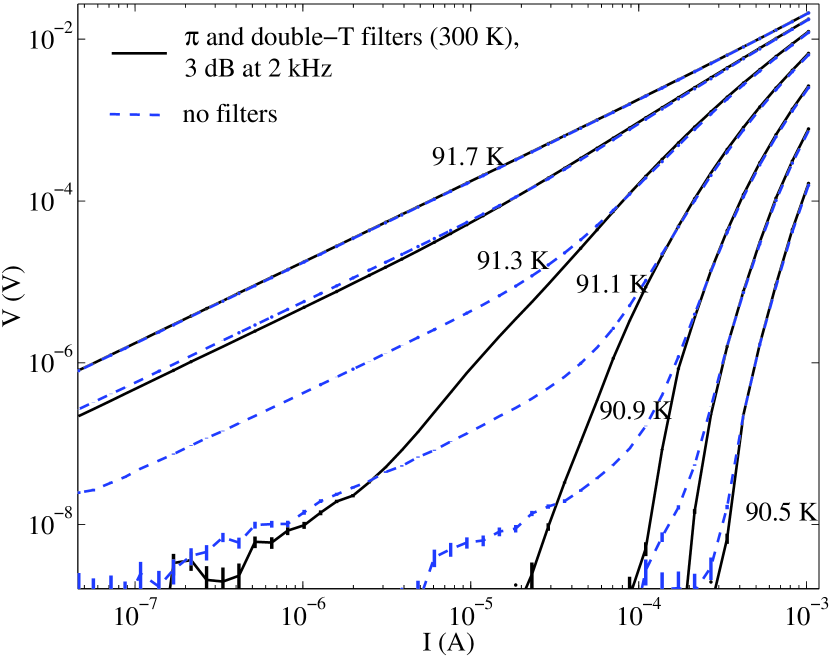
Figure 1: Two sets of $I-V$ curves for a 2100 Å thick film with bridge dimensions $8\times 40\ \mu$m². The solid lines are isotherms taken with low-pass $\pi$ filters (3 dB at 4 kHz) at the screened room wall and low-pass double-T filters (3 dB at 2 kHz) at the top of the probe. The dashed lines are isotherms taken without filtering. The isotherms are separated by 200 mK, and the error bars are shown (when larger than the lines). The highest-temperature isotherms (91.7 K) are ohmic, and fully in the normal state. In the transition region, we see (especially in the isotherms at 91.1 K and 90.9 K) that noise creates ohmic tails in non-linear signals.

In this figure, the highest-temperature isotherm (91.7 K) is in the normal state, and has a slope of one (indicating ohmic behavior, $V\sim I$). In the transition region, the effect of noise is dramatically apparent. The filtered isotherms (solid lines) and the unfiltered isotherms (dashed lines) overlap at high currents, as predicted by Eq. 3, indicating that the additional noise has no effect. At lower currents, however, the unfiltered isotherms deviate and become ohmic (same slope as the isotherm at 91.7 K), as expected from Eq. 5. This effect is most noticeable in the isotherms at 91.1 K and 90.9 K, where the non-linear isotherms become ohmic at low currents when the filters are removed.

It is also easy to see how these ohmic tails due to noise could be mistaken for ohmic tails due to the 3-D phase transition. The ohmic tail due to noise at 90.5 K drops below the resolution of our voltmeter (1 nV), thus the unfiltered isotherm appears non-linear. This transition from isotherms with an ohmic tail (91.1 K and 90.9 K) to (apparently) non-linear isotherms (90.5 K and below) is the same signature we expect from the phase transition. From the unfiltered isotherms alone, the conventional analysis of $I-V$ curves would lead us to say that $T_{c}\approx 90.5$ K, despite the fact that the ohmic tails at 91.1 K and 90.9 K are artifacts created by noise. Note also that the filtered and unfiltered isotherms are equally smooth. Once the noise reaches the sample, its response changes, thus the measured isotherm will appear smooth, regardless of how much noise is in the system.

In an attempt to further filter our leads, we added T filters and copper-powder filterscu-powder to the cold end of our probe, very close to the sample. Isotherms taken with warm filtering at the screened room wall and the top of the probe (solid lines in Fig. 1) were identical to isotherms taken with filters at the screened room wall, top of the probe, and at the cold end of the probe. Thus, the addition of cold filters did not improve the data. From this we conclude that the Johnson noise created in the probe wiring is not significant.

It is instructive to consider the effect of cold filters alone vs. warm filters alone. Because the 3 dB point of the T filters shifts to 70 kHz when cold, we can compare low-pass filters with different 3 dB points. Isotherms taken with all three filter configurations are shown in Fig. 2. From Fig. 2 it is obvious that a 3 dB point of 70 kHz is not low enough to filter the noise properly, although the difference between warm filters and cold filters is only obvious at 91.3 K.

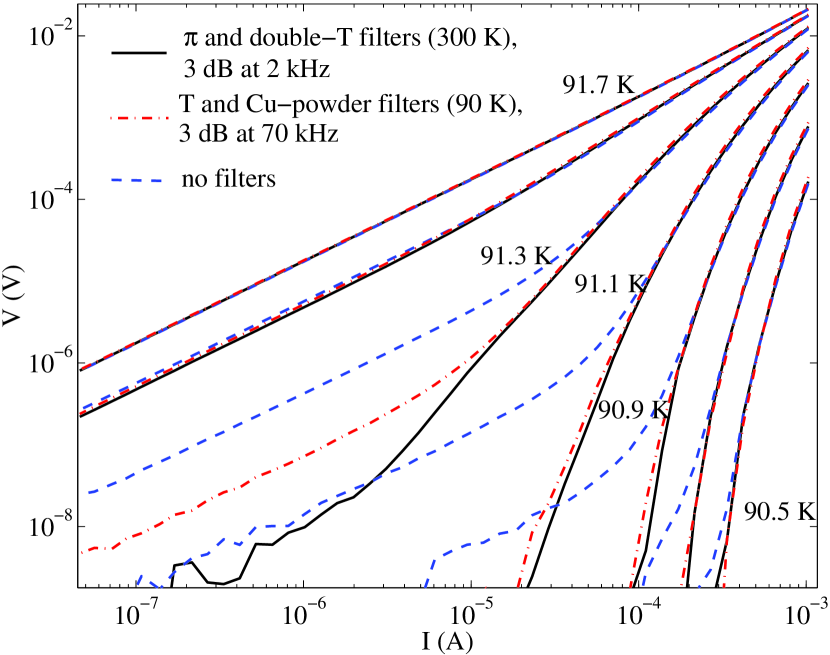
Figure 2: Three sets of $I-V$ curves for one sample. The solid lines and the dashed lines are the same isotherms from Fig. 1. The dotted-dashed lines are isotherms taken with T filters and copper-powder filters at the cold end of the probe (3 dB at 70 kHz). The isotherms are separated by 200 mK, and in this figure, the error bars are suppressed for clarity. We can see that a 3 dB point of 70 kHz is not low enough to filter the isotherm completely.

This result leads us to wonder whether even a 3 dB point of 2 kHz is low enough to properly filter the data. Commercial passive filters with a 3 dB point lower than 2 kHz are hard to find, but we can resolve this question using another method. The environment connected to the sample generates a certain amount of current noise, but the $I-V$ curves depend not on current but rather current density. Therefore, if we test 4-probe bridges of different widths, for a given amount of noise current, we can reduce the noise current density using wider bridges. We expect bridges of different widths to have similar $J-E$ curves, where $J$ is current density and $E$ electric field. However, if noise is still a problem, wider bridges should show different $E-J$ curves. We have measured bridges of different widths,me and have found that for typical filtering (3 dB at 2 kHz), the $E-J$ curves for bridges of different widths (and thus different noise current densities) are identical, indicating that our low-pass $\pi$ filters are sufficient filtering.

Additionally, we can take an isotherm and use Eq. 10 to estimate the amount of current noise required to create the ohmic tail. If we take the filtered isotherm at 91.3 K from Fig. 1, we find from the high currents $a\approx 1.55$ and $b\approx 10^{2.8}$ V/A^a. From the low currents, we find $R_{eff}\approx 0.7\ \Omega$. We can plug this in to Eq. 10, and find $\sigma_{I}\approx 1.3\ \mu$A, if the ohmic tail were caused by noise. We have measured the noise in our probe using a spectrum analyzer and found $\sigma_{I}\leq 10$ nA, far less than the estimate from Eq. 10, indicating that, with proper filtering, noise does not create the ohmic tails.

Finally, it is interesting to note that we can change the resistance of the ohmic tail at 91.3 K by adding noise in Fig. 2. We know from Eq. 8 that adding noise to a linear $I-V$ curve does not change the resistance. This result indicates that the underlying behavior at low currents of the 91.3 K isotherm must be non-linear! The ohmic tail that occurs even in the filtered data must result from some other effect. In Ref. me, , we argue that this occurs due to the finite thickness of our films.

We have shown, theoretically and experimentally, that the addition of current noise can create ohmic behavior at low currents in non-linear $I-V$ curves. We have also shown that, in our experimental setup, passive low-pass $\pi$ filters eliminated the effects of noise. However, without filters, it is easy to confuse ohmic tails generated by noise with ohmic tails expected from the phase transition, causing incorrect choices of $T_{c}$, $\nu$, and $z$. These exponents are expected to be universal, though many different exponents are reported in the literature. Filtering schemes are rarely explicitly mentioned in the literature, and thus current noise may be a possible explanation for the lack of consensus regarding the exponents.

The authors thank J. S. Higgins, D. Tobias, A. J. Berkley, S. Li, H. Xu, M. Lilly, Y. Dagan, H. Balci, M. M. Qazilbash, F. C. Wellstood, and R. L. Greene for their help and discussions on this work. We acknowledge the support of the National Science Foundation through Grant No. DMR-0302596.

References

- (1) C. J. Lobb, Phys. Rev. B 36, 3930 (1987).
- (2) D. S. Fisher, M. P. A. Fisher, and D. A. Huse, Phys. Rev. B 43, 130 (1991); D. A. Huse, D. S. Fisher, and M. P. A. Fisher, Nature 358, 553 (1992).
- (3) See Ref. doug, and the references therein for a short list of the many papers using curves to examine critical behavior.
- (4) R. H. Koch et al., Phys. Rev. Lett. 63, 1511 (1989); R. H. Koch, V. Foglietti, and M. P. A. Fisher, Phys. Rev. Lett. 64, 2586 (1990).
- (5) P.J.M Wöltgens, C. Dekker, R.H. Koch, B.W. Hussey, and A. Gupta, Phys. Rev. B 52, 4536 (1995); A. Sawa, Hirofumi Yamasaki, Y. Mawatari, H. Obara, M. Umeda, and S. Kosaka, Phys. Rev B 58, 2868 (1998).
- (6) N.-C. Yeh, W. Jiang, D. S. Reed, U. Kriplani and F. Holtzberg, Phys. Rev. B 47, 6146 (1992); N.-C. Yeh, D. S. Reed, W. Jiang, U. Kriplani, F. Holtzberg, A. Gupta, B. D. Hunt, R. P. Vasquez, M. C. Foote, and L. Bajuk, Phys. Rev. B 45, 5654 (1992).
- (7) C. Dekker, R.H. Koch, B. Oh and A. Gupta, Physica C 185-189, 1799 (1991); J.M. Roberts et al., Phys. Rev. B 49, 6890 (1994); T. Nojima et al., Czech. Jour. Phys. 46 Suppl. S3, 1713 (1996); K. Moloni, M. Friesen, S. Li, V. Souw, P. Metcalf, L. Hou, and M. McElfresh, Phys. Rev. Lett. 78, 3173 (1997).
- (8) H. Safar, P. L. Gammel, D. J. Bishop, D. B. Mitzi, and A. Kapitulnik, Phys. Rev. Lett. 68, 2672 (1992); Qiang Li, H. J. Wiesmann, M. Suenaga, L. Motowidlow, and P. Haldar, Phys. Rev. B 50, 4256 (1994); H. Yamasaki, K. Endo, S. Kosaka, M. Umeda, S. Yoshida, and K. Kajimura, Phys. Rev. B 50, 12959 (1994).
- (9) N. C. Yeh, W. Jiang, D. S. Reed, A. Gupta and F. Holtzberg, and A. Kussmaul, Phys. Rev. B 45 5710 (1992); J. M. Roberts, B. Brown, J. Tate, X. X. Xi, S. N. Mao, Phys. Rev. B 51 15281 (1995)
- (10) T. Klein, et. al, Phys. Rev. B 58, 12411 (1998).
- (11) S. Okuma and N. Kokubo, Phys. Rev. B 56 14138 (1997); S. Okuma, Y. Imamoto, and M. Morita, Phys. Rev. Lett. 86 3136, (2001)
- (12) S. N. Coppersmith, M. Inui, and P. B. Littlewood, Phys. Rev. Lett. 64, 2585 (1990); B. Brown, Phys. Rev. B 61, 3267 (2000); Z. L. Xiao, J. Häring, Ch. Heinzel, and P. Ziemann, Sol. State Comm. 95, 153 (1995); H. S. Bokil and A. P. Young, Phys. Rev. Lett. 74, 3021 (1995); C. Wengel and A. P. Young, Phys. Rev. B 54, R6869 (1996); H. Kawamura, J. Phys. Soc. Jpn. 69, 29 (2000);
- (13) D. R. Strachan, M. C. Sullivan, P. Fournier, S. P. Pai, T. Venkatesan and C. J. Lobb, Phys. Rev. Lett. 87, 067007 (2001); D. R. Strachan, M. C. Sullivan, and C. J. Lobb, Proc. SPIE 4811, 65-77 (2002).
- (14) J. M. Repaci, Ph.D. thesis, University of Marlyand, 1996; D. R. Strachan, Ph.D. thesis, University of Maryland, 2002; M. C. Sullivan, Ph.D. thesis, University of Maryland, 2004.
- (15) Eq. 4 is always true for any symmetric and antisymmetric , given that .
- (16) Again, Eq. 8 is true for any symmetric .
- (17) John M. Martinis, Michel H. Devoret, and John Clarke, Phys. Rev. B 35, 4682 (1987).
- (18) M. C. Sullivan, D. R. Strachan, T. Frederiksen, R. A. Ott, M. Lilly, and C. J. Lobb, Phys. Rev. B 69, 214524 (2004).