Field-induced phase transitions in a Kondo insulator

Abstract

We study the magnetic-field effect on a Kondo insulator by exploiting the periodic Anderson model with the Zeeman term. The analysis using dynamical mean field theory combined with quantum Monte Carlo simulations determines the detailed phase diagram at finite temperatures. At low temperatures, the magnetic field drives the Kondo insulator to a transverse antiferromagnetic phase, which further enters a polarized metallic phase at higher fields. The antiferromagnetic transition temperature $T_{c}$ takes a maximum when the Zeeman energy is nearly equal to the quasi-particle gap. In the paramagnetic phase above $T_{c}$, we find that the electron mass gets largest around the field where the quasi-particle gap is closed. It is also shown that the induced moment of conduction electrons changes its direction from antiparallel to parallel to the field.

I Introduction

There has been a continued interest in a class of compounds called Kondo insulators or heavy fermion semiconductors,ki which develop an insulating gap at low temperatures via strong correlation effects. ${\rm CeRhAs}$, ${\rm Ce_{3}Bi_{4}Pt_{3}}$, ${\rm YbB_{12}}$, and ${\rm SmB_{6}}$ are well known examples, which possess small gaps of the order of 1-100 meV in spin and charge excitations. The gap formation in Kondo insulators is attributed to the renormalized hybridization between a broad conduction band and a nearly flat $f$-electron band with strong correlations. In some Kondo insulators, enhanced antiferromagnetic (AF) correlations among localized $f$-moments dominate the Kondo singlet formation, resulting in an AF long-range order.ins Systems located around such magnetic instability provide hot topics in quantum critical phenomena.qcp

The application of a magnetic field to the Kondo insulators also realizes quantum critical phenomena, which have been investigated extensively. Experiments on ${\rm Ce_{3}Bi_{4}Pt_{3}},$ce ${\rm YbB_{12}},$yb and ${\rm SmB_{6}}$sm in high magnetic fields indicate closure of the Kondo-insulating gap, exemplifying a transition from the Kondo insulator to a correlated metal. If the Kondo insulator is in the proximity of magnetic instability, the local singlet formation gets weak, and the applied field may possibly trigger a phase transition to the AF ordered state before it becomes a metal.

The periodic Anderson model (PAM) at half filling may be a simplified model to describe the Kondo insulating phasehf and the AF phase, depending on the $c$-$f$ hybridization strength $V$ and the $f$-$f$ Coulomb interaction $U$. The magnetic instability of the PAM has been investigated by means of various methods such as slave-boson mean field theorypam_phase1 ; pam_ins ; pam_phase2 and dynamical mean field theory (DMFT). jarrell ; rozenberg ; dmft ; imai The effect of the magnetic field on the PAM has also been investigated,saso ; ono ; ohara ; mutou1 ; satoh ; meyer and the phase transition from the Kondo insulator to a paramagnetic metal, which is naively expected, has been discussed.

Recently, Beach et. al.beach have studied the magnetic-field effect on the two-dimensional Kondo lattice model using large-$N$ mean field theory and quantum Monte Carlo (QMC) simulations. Also, Milat et. al. have presented a mean field analysis of the PAM in the small $U$ region and QMC simulations of the Kondo lattice model.milat They have found that the magnetic field induces a second-order phase transition from the paramagnetic to the transverse AF phase in the Kondo insulator. Since these works have been concerned with the two-dimensional systems, it is desirable to extend the investigation to three-dimensional cases. Also, a detailed study including the paramagnetic phase at finite temperatures is expected to provide further interesting properties in the Kondo insulator in a magnetic field.

In this paper, we study field-induced AF phase transitions of the Kondo insulator in the whole temperature regime by using the PAM at half filling. By exploiting DMFT combined with the QMC method,qmc we show that a magnetic field induces a transverse AF order in the Kondo insulator. We also demonstrate that a correlated metallic state with characteristic properties emerges in the paramagnetic phase slightly above the AF transition temperature, when the Zeeman energy is nearly equal to the spin gap.

This paper is organized as follows. In the next section, we briefly mention the model and method, and show the phase diagram obtained by DMFT. In Sec.III, we explain the detail of the field-induced AF transitions, and discuss some remarkable properties in the paramagnetic phase. Brief summary is given in Sec. IV.

II Model and Phase Diagram

Let us begin with the periodic Anderson model with the Zeeman term,

$$H = -t\sum_{\left<i,j\right>,\sigma}c_{i\sigma}^{\dagger}c_{j\sigma}+V\sum_{i,\sigma}\left[c_{i\sigma}^{\dagger}f_{i\sigma}+\mathrm{h.c.}\right]$$

$$+ U\sum_{i}\left[n^{f}_{i\uparrow}-1/2\right]\left[n^{f}_{i\downarrow}-1/2\right]$$

$$- g\mu_{B}B\sum_{i}\left[S^{f}_{i,z}+S^{c}_{i,z}\right],$$

where $c_{i\sigma}$ ($f_{i\sigma}$) annihilates a conduction ($f$) electron on the $i$th site with spin $\sigma$, $n_{i\sigma}^{a}=a_{i\sigma}^{{\dagger}}a_{i\sigma}$ and $S^{a}_{i,z}=\frac{1}{2}(n_{i\uparrow}^{a}-n_{i\downarrow}^{a})$ with $a=c,f$. Here, $t$ is the nearest-neighbor hopping matrix in the conduction band (referred to as the $c$ band in the following). We consider the hyper-cubic lattice with a bipartite property in infinite dimensions. The bare density of states for $c$ electrons is Gaussian with the width $t^{*}$: $\rho_{0}(\varepsilon)=\exp[-(\varepsilon/t^{*})^{2}]/\sqrt{\pi t^{*2}}$. The magnetic field $B$ applied along the $z$ direction is coupled to both of the $c$ and $f$ electrons. We assume that the $g$ factors of the $c$ and $f$ electrons are the same, and set $g\mu_{B}=1$. These simplifications would not qualitatively change our conclusions.

DMFT is a powerful framework to study strongly correlated electron systems, e.g., the single-band Hubbard model,georges ; jarrell_shm ; zhang ; caffarel ; fisher ; kajueter ; bulla the two-band Hubbard model,rozenberg_thm ; held ; han ; maier ; momoi ; imai2 ; oudovenko ; florens ; koga the PAM,jarrell ; rozenberg ; imai ; saso ; mutou1 ; meyer ; tahvildar ; pruschke ; shimizu ; vidhyadhiraja ; ryouta ; mutou2 etc. This method is justified in the limit of large spatial dimensions and gives a rather good approximation even in three dimensions. In DMFT, the proper one-particle self-energy, which is independent of the momentum, is obtained via an effective impurity model embedded in a self-consistently determined medium. The DMFT treatment of the PAM is summarized in Appendix A. We solve the effective impurity model using the QMC method with the Trotter time slices, $\Delta\tau=\beta/L\leq 0.25$ ($\beta=1/T$). The number of QMC sweeps is $3.2\times 10^{6}$ in each DMFT iteration loop. We use the typical parameters $U/t^{*}=2.0$ and $V/t^{*}=0.6$ in the following calculation. For these parameters, the ground state at zero field is a paramagnetic Kondo insulator, as shown by Jarrell et. al.jarrell It is convenient to express the energy normalized by the zero field value of quasi-particle gap, $\Delta_{0}\sim 0.145t^{*}$, which is estimated from the $f$-electron spectral function at $T/t^{*}=1/30$ (see Fig. 3).

We first give an overview of the phase diagram obtained in this paper, which is shown in Fig.1. At weak fields, the system is in the Kondo insulating phase characterized by the gap formation of quasi-particle states, which is smoothly connected to the high-temperature paramagnetic phase. Beyond a certain critical field, there is a second-order phase transition from the paramagnetic phase to the low-temperature AF phase with the decrease of temperature. The AF phase possesses a long-range order in the $xy$ plane, namely, the transverse AF order.

It is seen that the transition temperature $T_{c}$ takes a maximum, when the Zeeman energy is nearly equal to the spin gap $B\sim 2\Delta_{0}$. Around this field, we find remarkable properties in the paramagnetic phase just above $T_{c}$: they are characterized by two crossover fields, $B_{G}$ and $B_{K}$. The quasi-particle gap is closed for fields higher than $B_{G}$. At $B_{K}$, the magnetization of the $c$ electrons changes its sign. The region surrounded by $T_{c}$, $B_{G}$ and $B_{K}$ may be referred to as a ‘Kondo metal’, where the quasi-particle gap is closed but the Kondo correlations are still dominant to produce the strong renormalization effects accompanied by the large mass enhancement. As a result, this Kondo-metal region exhibits interesting properties coming from the competition of the Kondo correlations, the AF instability, etc.

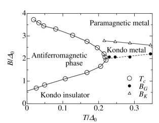
Figure 1: Phase diagram of the PAM on the hypercubic lattice in infinite dimensions. The parameters are chosen as $U=2.0$ and $V=0.6$. The second-order AF transition temperature $T_{c}$ is indicated by open circles. Two fields $B_{G}$ and $B_{K}$ characterize the crossover behavior related to the gap closing and the change in the magnetization process, respectively. The region denoted as a Kondo metal possesses interesting physical properties different from ordinary heavy electrons, see text.

III Detail of the Results

We now explain how the above phase diagram is obtained in the DMFT framework. We first investigate the field-induced AF transitions, and then discuss some characteristic properties in the paramagnetic phase.

III.1 Phase transitions

An AF transition is signaled by the divergence of the staggered spin susceptibility $\chi_{xx}(\mathbf{Q})$ with $\mathbf{Q}=[\pi,\pi,\ldots]$, where the suffix $x$ denotes the direction perpendicular to the field. In DMFT, we can calculate this quantity via the impurity model, since the irreducible vertex function as well as the self-energy is independent of the momentum in infinite dimensions.jarrell The detail of the calculation is summarized in Appendix B.

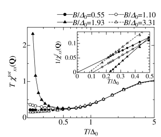
Figure 2: Temperature dependence of the total staggered susceptibility $\chi^{tot}_{xx}(\mathbf{Q})$ with $\mathbf{Q}=[\pi,\pi,\ldots]$. Inset shows the inverse of the susceptibility for $f$ electrons $\chi^{f}_{xx}(\mathbf{Q})$. Both of $\chi^{tot}_{xx}(\mathbf{Q})$ and $\chi^{f}_{xx}(\mathbf{Q})$ diverge at the same critical temperature. $\chi^{f}_{xx}(\mathbf{Q})$ is well fitted with the form $1/\chi^{f}_{xx}(\mathbf{Q})\propto T-T_{c}$, which enables us to determine the transition temperature $T_{c}$ by a proper extrapolation procedure.

In Fig. 2, the staggered spin susceptibility $T\chi^{tot}_{xx}(\mathbf{Q})$ is plotted as a function of temperature for different magnetic fields. In the DMFT framework, the susceptibility exhibits mean-field behavior, $\chi_{xx}(\mathbf{Q})\propto[T-T_{c}]^{-1}$. Thus, we evaluate the transition temperature rather accurately by extrapolating the inverse susceptibility to zero as a function of $T$, as shown in the inset of Fig. 2. The transition temperature $T_{c}$ thus obtained for various values of $B$ is plotted in the phase diagram shown in Fig. 1. The magnetic field triggers a phase transition from the paramagnetic Kondo insulator to the transverse AF ordered state. The critical field between the Kondo insulator and the AF insulator is estimated as $B\sim 0.56\Delta_{0}$ at $T=0$. In our calculation, it is somewhat difficult to precisely determine the higher critical field separating the AF phase and the paramagnetic metallic phase at $T=0$, since the signal of antiferromagnetism appears at very low temperature with increasing $B/\Delta_{0}$. Milat et. al. concluded that the AF state should persist up to the fully polarized state because of perfect nesting.milat Our numerical results support their conclusion, although such a transition would occur at extremely low temperatures in the high field regime. It is instructive to note that the transition temperature $T_{c}$ takes a maximum value $T_{c}\sim 0.22\Delta_{0}$ around the field $B\sim 1.93\Delta_{0}$, which is almost the same as the spectral gap, $2\Delta_{0}$. We will see that this value of field is close to two typical crossover fields discussed below.

III.2 Heavy-fermion behavior in paramagnetic phase

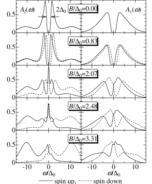
Figure 3: Spectral functions of $f$ (left) and $c$ (right) electrons at $T=0.23\Delta_{0}$ for different values of $B/\Delta_{0}$. The energy scale $\Delta_{0}$ is determined by the distance between zero frequency and the frequency which takes the half value of the first peak in the $f$-electron spectral function at zero field.

We obtain dynamical quantities by applying the maximum entropy method (MEM) to the imaginary-time QMC data computed with DMFT. In Fig. 3, we show the one-particle spectral functions for the $c$ and $f$ electrons, $A_{c\uparrow,\downarrow}(\omega)$ and $A_{f\uparrow,\downarrow}(\omega)$, at $T=0.23\Delta_{0}$ for different magnetic fields. Note that the system is in the paramagnetic phase for any magnetic fields at this temperature. One can see in this figure how the magnetic filed closes the quasi-particle gap and then induces correlated metallic states. At $B=0$, the well-defined insulating gap exists both for $f$ and $c$ electrons. As the field is increased ($B/\Delta_{0}=0.83$), the peak structure existing beside the gap is slightly shifted in the presence of the Zeeman splitting. For $B/\Delta_{0}\sim 2$, the spectral gap almost disappears. A remarkable point in this case is that $f$ electrons get another sharp peak structure around $\omega=0$, as seen for the third panel in Fig. 3. This implies that strong Kondo correlations still persist even in such fields, driving the system to a correlated metallic state (Kondo metal in Fig. 1) immediately after the quasi-particle gap is closed by the field. If the field is further increased, such a sharp quasi-particle peak disappears, and the system gradually changes to an ordinary paramagnetic metal with the spin polarization.

In order to see the above characteristics clearly, we show the $f$-electron spectral weight at the Fermi level, $A_{f}(0)=[A_{f_{\uparrow}}(0)+A_{f_{\downarrow}}(0)]/2$, in Fig. 4 (a) as a function of the magnetic field at different temperatures. It may be legitimate to define the crossover field $B_{G}$ characterizing the gap-closing by the field where $A_{f}(0)$ takes its maximum as a function of $B$. The crossover field thus estimated, $B_{G}\simeq 2\Delta_{0}$, is consistent with the known results that the spin gap is nearly equal to the quasi-particle gap in infinite dimensions.jarrell ; mutou2 It is seen that $B_{G}$ is almost independent of the temperature in the range shown in Fig.1. As a reference, in Fig. 4 (b) we show the numerical derivative of the $f$-electron self-energy, $Z$, which would correspond to the inverse of the mass-enhancement factor at low temperatures. It is seen that $Z^{-1}$ indeed takes its maximum around the field $B_{G}$, which seems consistent with the development of the sharp quasi-particle peak in Fig. 3. However, one notices that the mass enhancement (i.e. development of the sharp peak) observed around $B/\Delta_{0}\sim 2$ in Fig. 3 is larger than that in Fig. 4(b). This difference comes from our numerical differentiation procedure with discrete frequency in Fig. 4(b), where we have naively used the formula in the Matsubara form, $Z={\mathrm{I}\mathrm{m}}\Sigma(\omega_{0})/\omega_{0}$ with $\omega_{0}=\pi T$. This formula may not pick up the sharp structure of the spectrum around $B/\Delta_{0}\sim 2$ in Fig. 3. Therefore, the actual mass enhancement should be somewhat larger than that displayed in Fig. 4(b).

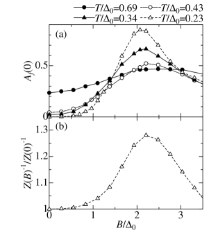
Figure 4: (a) The $f$-electron spectral function at the Fermi level $A_{f}(0)$ as a function of $B/\Delta_{0}$, which is used to determine $B_{G}$; (b) the derivative of the $f$-electron self-energy $Z(B)^{-1}$ at $T=0.23\Delta_{0}$ normalized by its zero-field value $Z(0)^{-1}(\simeq 2)$. Here $Z$ is computed numerically by the formula $Z={\mathrm{I}\mathrm{m}}\Sigma(\omega_{0})/\omega_{0}$ with $\omega_{0}=\pi T$.

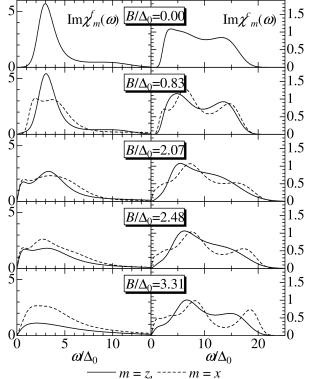
Figure 5: Dynamical spin-correlation function, $\mathrm{Im}\chi^{m}_{\alpha}(\omega)$, for $f$ (left panel) and $c$ (right panel) electrons at $T/\Delta_{0}=0.23$ for different values of $B/\Delta_{0}$. Solid (broken) lines represent the $z$- ($x$-) component of the spin correlation function, where the $z$ axis is parallel to the applied field.

We further calculate the dynamical spin-correlation function to directly observe the magnetic-field effects on spin excitations. The imaginary-time spin-correlation function $\chi^{m}_{\alpha}(\tau)$, defined as $\chi^{m}_{\alpha}(\tau)=\left\langle\mathrm{T}_{\tau}S_{i,\alpha}^{m}\left(\tau\right)S_{i,\alpha}^{m}\left(0\right)\right\rangle$ with $m=c,f$ and $\alpha=z,x$, is calculated by the QMC method and is analytically continued to the real frequency with MEM. In Fig. 5, we show the field dependence of $\mathrm{Im}\chi^{m}_{\alpha}(\omega)$ at a given temperature, $T/\Delta_{0}=0.23$, slightly larger than the maximum AF transition temperature.

At zero field, there are two characteristic features in the dynamical spin-correlation functions. One is a low-energy peak (shoulder) structure in $\mathrm{Im}\chi_{\alpha}^{f}(\omega)$ ($\mathrm{Im}\chi_{\alpha}^{c}(\omega)$) due to spin-triplet excitations, which determine the size of the spin gap. The other is a broad continuum in the high-energy region due to the dispersion of $c$ electrons, which features a higher-energy hump in $\mathrm{Im}\chi_{\alpha}^{c}(\omega)$. When a magnetic field is introduced, the spin-triplet excitations split into three distinct excitations specified by $S_{z}^{tot}$. At $B/\Delta_{0}=0.83$, the magnetic field little affects the shape of $\mathrm{Im}\chi_{z}^{f,c}(\omega)$, whereas it splits the low-energy peak of $\mathrm{Im}\chi_{x}^{f,c}(\omega)$ into two sub-peaks. The results are naturally understood, because the triplet excitations observed in $\mathrm{Im}\chi_{z}^{f,c}(\omega)$ ($\mathrm{Im}\chi_{x}^{f,c}(\omega)$) are those with $S_{z}^{tot}=0$ ($S_{z}^{tot}=\pm 1$): the latter causes the splitting in the spin excitation spectrum. If the field is further increased, the spin gap disappears around $B/\Delta_{0}\sim 2$, making the Kondo singlet state unstable. Note that around this field, $\mathrm{Im}\chi_{z}^{f}(\omega)$ develops another hump structure around $\omega=0$, which is consistent with the fact that heavy-fermion states with the enhanced mass appear in the one-particle spectrum (Fig. 3). Another noticeable point is that $\mathrm{Im}\chi_{z}^{c}(\omega)$ does not increase its weight around $\omega=0$, although $\mathrm{Im}\chi_{x}^{c}(\omega)$ as well as $\mathrm{Im}\chi_{z,x}^{f}(\omega)$ already has a reasonable weight (see data at $B/\Delta_{0}=2.07$). Furthermore, $\mathrm{Im}\chi_{z}^{c}(\omega)$ eventually develops a shoulder-like structure around $\omega=0$ at $B/\Delta_{0}=3.31$, where the heavy-fermion behavior in $\mathrm{Im}\chi_{z}^{f}(\omega)$ is already suppressed. In this way, the $z$-component spin excitations of $c$ electrons exhibit unusual behavior around the field $B/\Delta_{0}=2\sim 3$.

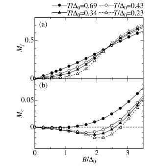
Figure 6: The magnetization process of $f$ (a) and $c$ (b) electrons. $M_{f}$ and $M_{c}$ are defined by $M_{f}=\langle n_{f\uparrow}-n_{f\downarrow}\rangle$ and $M_{c}=\langle n_{c\uparrow}-n_{c\downarrow}\rangle$.

To make the above point clear, we turn to another interesting crossover behavior denoted by the line $B_{K}$ (see Fig.1) in the paramagnetic phase above $T_{c}$. This line is determined by the change in the magnetization process for $c$ electrons. Shown in Figs. 6 (a) and (b) are the magnetization of $f$ and $c$ electrons at several different temperatures. It is found that the magnetization of $f$ electrons is always positive, while that of $c$ electrons is negative for weak fields and gets positive beyond a certain magnetic field. We define $B_{K}$ by the magnetic field at which the magnetization of $c$ electrons changes its sign. This field $B_{K}$ roughly corresponds to the strength of the local singlet formation. At weak fields, the Kondo effect is still dominant to align the spins of $c$ and $f$ electrons in the opposite directions, which may give rise to the negative magnetization in $c$ electrons. Such nonmonotonic behavior is also seen in the spectral function of $c$ electrons in Fig. 3. The spectral function of $c$ electrons with up spin is shifted to the low-energy side, while its weight is considerably suppressed. These results are also consistent with what we have observed in the small-$\omega$ behavior of $\mathrm{Im}\chi^{x}_{c}(\omega)$ for $B/\Delta_{0}=2\sim 3$ in Fig. 5.

Summarizing the results found in the normal phase, we can say that around the field where $T_{c}$ takes a maximum, various correlation effects such as the Kondo-gap formation, the AF instability, etc. compete with each other, yielding characteristic properties in correlated electrons. Such features are different from ordinary heavy fermions without magnetic fields.

IV Summary

We have investigated the effects of the magnetic field on the Kondo insulator by applying DMFT to the PAM at finite temperatures. There are several characteristic features in the phase diagram. At low temperatures, we have observed the quantum phase transition from the Kondo insulator to the transverse AF phase, in accordance with the results obtained in the two-dimensional case. We have also found some remarkable properties in the paramagnetic regime. Namely, in the paramagnetic phase close to the maximum AF transition temperature, heavy-fermion states with the enhanced mass are realized, where the competition of the magnetic field and the Kondo correlations results in characteristic features in the one-particle spectrum, the dynamical spin susceptibility and the magnetization process. It may be interesting to experimentally investigate static as well as dynamical properties in this region. Such investigation may provide a unique example of field-induced heavy-fermion states without phase transitions.

Appendix A Formulation of DMFT

In this Appendix, we summarize the DMFT formulation of the PAM.dmft ; jarrell ; rozenberg In DMFT, the original lattice model is mapped onto an effective impunity model with the effective medium determined self-consistently. This medium is described in terms of a cavity Green’s function ${\bf\cal G}(i\omega_{n})$, which represents the motion of correlated electrons on all sites except an impurity site. The local Green’s function ${\bf G}(i\omega_{n})$ is then expressed in terms of the momentum-independent self-energy $\Sigma(i\omega_{n})$ and the cavity Green’s function ${\cal G}(i\omega_{n})$ as

$${\bf G}^{\sigma}(i\omega_{n})=\left[{\bf\cal G}^{\sigma}(i\omega_{n})^{-1}-{\bf\Sigma}^{\sigma}(i\omega_{n})\right]^{-1},$$ (1)

where the Green’s functions and the self-energy are expressed in the matrix form,

$${\bf G}^{\sigma}(i\omega_{n}) = \left[\begin{array}[]{cc}G_{cc}^{\sigma}(i\omega_{n})&G_{cf}^{\sigma}(i\omega_{n})\\ G_{fc}^{\sigma}(i\omega_{n})&G_{ff}^{\sigma}(i\omega_{n})\end{array}\right],$$ (4)

$${\bf\cal G}^{\sigma}(i\omega_{n}) = \left[\begin{array}[]{cc}{\cal G}_{cc}^{\sigma}(i\omega_{n})&{\cal G}_{cf}^{\sigma}(i\omega_{n})\\ {\cal G}_{fc}^{\sigma}(i\omega_{n})&{\cal G}_{ff}^{\sigma}(i\omega_{n})\end{array}\right],$$ (7)

$${\bf\Sigma}^{\sigma}(i\omega_{n}) = \left[\begin{array}[]{cc}0&0\\ 0&\Sigma^{\sigma}_{f}(i\omega_{n})\end{array}\right].$$ (10)

On the other hand, the local Green’s function $G(i\omega_{n})$ can be written as

$$G^{\sigma}(i\omega_{n}) = \int d\varepsilon\frac{\rho_{0}(\varepsilon)}{\xi^{\sigma}(i\omega_{n},\varepsilon)}\left[\begin{array}[]{cc}\xi_{f}^{\sigma}(i\omega_{n})&V\\ V&\xi_{c}^{\sigma}(i\omega_{n},\varepsilon)\end{array}\right]$$ (13)

with

$$\xi_{c}^{\sigma}\left(i\omega_{n},\varepsilon\right) = i\omega_{n}+\frac{1}{2}\sigma g\mu_{B}B-\varepsilon,$$ (15)

$$\xi_{f}^{\sigma}\left(i\omega_{n}\right) = i\omega_{n}-\frac{U}{2}+\frac{1}{2}\sigma g\mu_{B}B-\Sigma_{f}\left(i\omega_{n}\right),$$ (16)

$$\xi^{\sigma}\left(i\omega_{n},\varepsilon\right) = \xi_{c}^{\sigma}\left(i\omega_{n},\varepsilon\right)\xi_{f}^{\sigma}\left(i\omega_{n}\right)-V^{2}.$$ (17)

By solving equations (1) and (LABEL:lattice) self-consistently, we can discuss the effects of electron correlations on local properties in the PAM. In this paper, we obtain the imaginary-time Green’s function $G^{\sigma}(\tau)$ by solving the impurity problem with the QMC method.qmc

Appendix B Magnetic Susceptibility

To discuss the instability to an AF ordered phase, it is necessary to obtain the momentum-dependent susceptibility $\chi_{xx}(\mathbf{q})$ in the PAM. Here, we explain how this quantity is formulated in the framework of DMFT.dmft ; jarrell

We first consider the local two-particle propagator in the effective impurity system,

$$\chi_{+-i}^{f}\left(\tau_{1},\tau_{2},\tau_{3},\tau_{4}\right)$$ (18)

$$= \left\langle\mathrm{T}_{\tau}f^{\dagger}_{i\uparrow}\left(\tau_{1}\right)f_{i\downarrow}\left(\tau_{2}\right)f^{\dagger}_{i\downarrow}\left(\tau_{3}\right)f_{i\uparrow}\left(\tau_{4}\right)\right\rangle,$$

$$\chi_{-+i}^{f}\left(\tau_{1},\tau_{2},\tau_{3},\tau_{4}\right)$$ (19)

$$= \left\langle\mathrm{T}_{\tau}f^{\dagger}_{i\downarrow}\left(\tau_{1}\right)f_{i\uparrow}\left(\tau_{2}\right)f^{\dagger}_{i\uparrow}\left(\tau_{3}\right)f_{i\downarrow}\left(\tau_{4}\right)\right\rangle.$$

We obtain the vertex function $\Gamma(i\nu_{l}=0;i\omega_{m},i\omega_{n})$ by solving the Bethe-Salpeter equation,

$$\chi^{f}_{i}=\chi^{f0}_{i}+\chi^{f0}_{i}\Gamma\chi^{f}_{i},$$ (20)

where $\chi^{f0}_{i}$ is the non-interacting part of the local two-particle propagator,

$$\chi^{f0}_{i}\left(i\nu_{l}=0;i\omega_{m},i\omega_{n}\right)=-\frac{\delta_{m,n}}{\beta}G_{ff}^{\uparrow}\left(i\omega_{n}\right)G_{ff}^{\downarrow}\left(i\omega_{n}\right).$$ (21)

By using the vertex function $\Gamma$, we obtain the two-particle propagator for correlated $f$-electrons in the lattice system,

$$\chi^{f}_{\mathbf{q}}=\chi^{f0}_{\mathbf{q}}+\chi^{f0}_{\mathbf{q}}\Gamma\chi^{f}_{\mathbf{q}},$$ (22)

where $\chi^{f0}_{\mathbf{q}}$ is the bare two-particle propagator in the lattice system given by,

$$\chi^{f0}_{+-{\mathbf{q}}}\left(i\nu_{l}=0;i\omega_{m},i\omega_{n}\right)$$

$$=-\frac{\delta_{n,m}}{N\beta}\sum_{\mathbf{k}}G^{ff}_{\mathbf{k}\uparrow}\left(i\omega_{n}\right)G^{ff}_{\mathbf{k}+\mathbf{q}\downarrow}\left(i\omega_{n}\right),$$ (23)

$$\chi^{f0}_{-+\mathbf{q}}\left(i\nu_{l}=0;i\omega_{m},i\omega_{n}\right)$$

$$=-\frac{\delta_{n,m}}{N\beta}\sum_{\mathbf{k}}G^{ff}_{\mathbf{k}\downarrow}\left(i\omega_{n}\right)G^{ff}_{\mathbf{k}+\mathbf{q}\uparrow}\left(i\omega_{n}\right).$$ (24)

Equations (23) and (24) can be rewritten as

$$\chi_{+-\mathbf{q}}^{f0}(i\nu_{l}=0;i\omega_{m},i\omega_{n})=$$

$$-\frac{\delta_{m,n}}{\beta}\int dx_{1}dx_{2}\Delta_{\mathbf{q}}(x_{1},x_{2})\frac{\xi_{c}^{\uparrow}(i\omega_{m},x_{1})\xi_{c}^{\downarrow}(i\omega_{m},x_{2})}{\xi^{\uparrow}(i\omega_{m},x_{1})\xi^{\downarrow}(i\omega_{m},x_{2})},$$

$$\chi_{-+\mathbf{q}}^{f0}(i\nu_{l}=0;i\omega_{m},i\omega_{n})=$$

$$-\frac{\delta_{m,n}}{\beta}\int dx_{1}dx_{2}\Delta_{\mathbf{q}}(x_{1},x_{2})\frac{\xi_{c}^{\downarrow}(i\omega_{m},x_{1})\xi_{c}^{\uparrow}(i\omega_{m},x_{2})}{\xi^{\downarrow}(i\omega_{m},x_{1})\xi^{\uparrow}(i\omega_{m},x_{2})},$$

with the two-particle density of states $\Delta_{q}(x_{1},x_{2})$ defined as

$$\Delta_{\mathbf{q}}(x_{1},x_{2})=\frac{1}{N}{\sum_{\mathbf{k}}}\delta(x_{1}-\varepsilon_{\mathbf{k}})\delta(x_{2}-\varepsilon_{\mathbf{k}+\mathbf{q}}).$$ (27)

If we focus on the center or the corner of the Brillouin zone, this function is reduced to the simpler form,

$$\Delta_{\mathbf{q}}(x_{1},x_{2})=\left\{\begin{array}[]{cl}\delta(x_{1}-x_{2})\rho_{0}(x_{1}),&\mathbf{q}=\left[0,0,\ldots\right]\\ \delta(x_{1}+x_{2})\rho_{0}(x_{1}),&\mathbf{q}=\left[\pi,\pi,\ldots\right]\end{array}\right..$$ (30)

Using the above equations, we can calculate the momentum-dependent two-particle propagator $\chi_{\mathbf{q}}^{f}(i\nu_{l}=0;i\omega_{m},i\omega_{n})$. We then obtain the static susceptibility,

$$\chi^{f}(\mathbf{q})=\frac{1}{\beta}\sum_{m,n}\chi^{f}_{\mathbf{q}}(i\nu_{l}=0;i\omega_{m},i\omega_{n}).$$ (32)

The total two-particle propagator in the lattice system, defined as $\chi_{\mathbf{q}}^{tot}=\chi_{\mathbf{q}}^{c}+\chi_{\mathbf{q}}^{cf}+\chi_{\mathbf{q}}^{fc}+\chi_{\mathbf{q}}^{f},$ can be expressed by that for correlated $f$-electrons $\chi^{f}_{\mathbf{q}}$ as

$$\chi_{\mathbf{q}}^{tot} = \chi_{\mathbf{q}}^{c0}-\chi_{\mathbf{q}}^{cf0}\left(\chi_{\mathbf{q}}^{f0}\right)^{-1}\chi_{\mathbf{q}}^{fc0}$$

$$+ \left[{\mathbf{I}}+\chi_{\mathbf{q}}^{cf0}\left(\chi_{\mathbf{q}}^{f0}\right)^{-1}\right]\chi_{\mathbf{q}}^{f}\left[{\mathbf{I}}+\left(\chi_{\mathbf{q}}^{f0}\right)^{-1}\chi_{\mathbf{q}}^{fc0}\right],$$

where ${\mathbf{I}}$ the unit matrix, and $\chi_{\mathbf{q}}^{c0}(i\nu_{l}=0;i\omega_{m},i\omega_{n})$ and $\chi_{\mathbf{q}}^{cf0}(i\nu_{l}=0;i\omega_{m},i\omega_{n})$ are the $c$-$c$ and $c$-$f$ elements of the bare two-particle propagator, which are obtained in the same way as $\chi_{\mathbf{q}}^{f0}(i\nu_{l}=0;i\omega_{m},i\omega_{n})$. We then obtain the total static-susceptibility $\chi^{tot}(\mathbf{q})$, summing over the Matsubara frequency in $\chi_{\mathbf{q}}^{tot}(i\nu_{l}=0;i\omega_{m},i\omega_{n})$.

References

- (1) P. S. Riseborough, Adv. Phys, 49, 257 (2000).
- (2) T. E. Mason, G. Aeppli, A. P. Ramirez, K. N. Clausen, C. Broholm, N. Stücheli, E. Bucher and T. T. M. Palstra, Phys. Rev. Lett. 69, 490 (1992); H. Kadowaki, T. Sato, H. Yoshizawa, T. Ekino, T. Takabatake, H. Fujii, L. P. Regnault and Y. Isikawa, J. Phys. Soc. Jpn. 63, 2074 (1994).
- (3) H. v. Lohneysen, J. Phys.: Condens. Matter 8, 9689 (1996); G. R. Stewart, Rev. Mod. Phys. 73, 794 (2001); Q. Si, S. Rabello, K. Ingersent and J. L. Smith, Nature 413 (2000).
- (4) M. Jaime, R. Movshovich, G. R. Stewart, W. P. Beyermann, M. G. Berisson, M. F. Hundley, P. C. Canfield and J. L. Sarrao, Nature 405, 160 (2000).
- (5) K. Sugiyama, F. Iga, M. Kasaya, T. Kasuya, and M. Date, J. Phys. Soc. Jpn. 57, 3946 (1988).
- (6) J. C. Cooley, C. H. Mielke, W. L. Hults, J. D. Goettee, M. M. Honold, R. M. Modler, A. Lacerda, D. G. Rickel and J. L. Smith, J. Supercond. 12, 171 (1999).
- (7) N. Grewe and F. Steglich, Handbook on the Physics and Chemistry of Rare Earths, edited by K. A. Gschneidner, Jr. and L. Eyring (North-Holland, Amsterdam, 1991), Vol. 14, p. 343.
- (8) V. Dorin and P. Schlottmann, Phys. Rev. B 46, 10800 (1992).
- (9) P. S. Riseborough, Phys. Rev. B 45, 13984 (1992).
- (10) R. Doradziński and J. Spalek, Phys. Rev. B 58, 3293 (1998).
- (11) M. Jarrell, H. Akhlaghpour, T. Pruschke Phys. Rev. Lett. 70, 1670 (1993); M. Jarrell Phys. Rev. B 51, 7429 (1995).
- (12) M. J. Rozenberg, Phys. Rev. B 52, 7369 (1995).
- (13) A. Georges, G. Kotliar, W. Krauth and M. J. Rozenberg, Rev. Mod. Phys. 68, 13 (1996).
- (14) Y. Imai and N. Kawakami, Acta. Phys. Pol. B 34, 779 (2003).
- (15) T. Saso, J. Phys. Soc. Jpn. 66, 1175 (1995); T. Saso and M. Itoh, Phys. Rev. B 53, 6877 (1996); T. Saso and H. Harima, J. Phys. Soc. Jpn. 72, 1131 (2003).
- (16) Y. Ōno, J. Phys. Soc. Jpn. 67, 2197 (1998).
- (17) K. Ohara, K. Hanzawa and K. Yosida, J. Phys. Soc. Jpn. 68, 521 (1999).
- (18) T. Mutou, Phys. Rev. B 62, 15589 (2000).
- (19) H. Satoh and F. J. Ohkawa, Phys. Rev. B 63, 184401 (2001).
- (20) D. Meyer and W. Nolting, Phys. Rev. B 64, 52402 (2001).
- (21) K. S. D. Beach, P. A. Lee and P. Monthoux, Phys. Rev. Lett. 92, 26401 (2004).
- (22) I. Milat, F. Assaad and M. Sigrist, Eur. Phys. J. B, 38, 571 (2004).
- (23) J. E. Hirsch and R. M. Fye, Phys. Rev. Lett. 56, 2521 (1986).
- (24) A. Georges and G. Kotliar, Phys. Rev. B 45, 6479 (1992).
- (25) M. Jarrell, Phys. Rev. Lett. 69, 168 (1992).
- (26) X. Y. Zhang, M. J. Rozenberg, and G. Kotliar, Phys. Rev. Lett. 70, 1666 (1993).
- (27) M. Caffarel and W. Krauth, Phys. Rev. Lett. 72, 1545 (1994).
- (28) D. S. Fisher, G. Kotliar, and G. Moeller, Phys. Rev. B 52, 17112 (1995).
- (29) H. Kajueter and G. Kotliar, Phys. Rev. Lett. 77, 131 (1996).
- (30) R. Bulla, Phys. Rev. Lett. 83, 136 (1999).
- (31) M. J. Rozenberg, Phys. Rev. B 55, R4855 (1997).
- (32) K. Held and D. Vollhardt, Eur. Phys. J. B 5, 473 (1998).
- (33) J. E. Han, M. Jarrell, and D. L. Cox, Phys. Rev. B 58, R4199 (1998).
- (34) Th. Maier, M. B. Zölfl, Th. Pruschke, and J. Keller, Eur. Phys. J. B 19, 377 (1999).
- (35) T. Momoi and K. Kubo, Phys. Rev. B 58, R567 (2000).
- (36) Y. Imai and N. Kawakami, J. Phys. Soc. Jpn. 70, 2365 (2001).
- (37) V. S. Oudovenko and G. Kotliar, Phys. Rev. B 65, 075102 (2002).
- (38) S. Florens, A. Georges, G. Kotliar and O. Parcollet, Phys. Rev. B 66, 205102 (2002).
- (39) A. Koga, Y. Imai, and N. Kawakami, Phys. Rev. B 66, 165107 (2002); A. Koga, T. Ohashi, Y. Imai, S. Suga and N. Kawakami, J. Phys. Soc. Jpn. 72, 1306 (2003); A. Koga, N. Kawakami, T. M. Rice and M. Sigrist, Phy. Rev. Lett. 92, 216402 (2004).
- (40) T. Mutou and D. Hirashima, J. Phys. Soc. Jpn. 63, 4475(1994); 64, 4799 (1995).
- (41) A. N. Tahvildar-Zadeh, M. Jarrell and J. K. Freericks, Phys. Rev. B 55, R3332 (1997);
- (42) Th. Pruschke, R. Bulla, M. Jarrell, Phys. Rev. B 61, 12799 (2000).
- (43) Y. Shimizu, O. Sakai and A. C. Hewson, J. Phys. Soc. Jpn. 69, 1777 (2000).
- (44) N. S. Vidhyadhiraja, V. E. Smith, D. E. Logan and H. R. Krishnamurthy, J. Phys.: Condens. Matter 15, 4045 (2003).
- (45) R. Sato, T. Ohashi, A. Koga and N. Kawakami, cond-mat/0404553