An associative network with spatially organized connectivity

Abstract

We investigate the properties of an autoassociative network of threshold-linear units whose synaptic connectivity is spatially structured and asymmetric. Since the methods of equilibrium statistical mechanics cannot be applied to such a network due to the lack of a Hamiltonian, we approach the problem through a signal-to-noise analysis, that we adapt to spatially organized networks. The conditions are analyzed for the appearance of stable, spatially non-uniform profiles of activity with large overlaps with one of the stored patterns. It is also shown, with simulations and analytic results, that the storage capacity does not decrease much when the connectivity of the network becomes short range. In addition, the method used here enables us to calculate exactly the storage capacity of a randomly connected network with arbitrary degree of dilution.

1 Introduction

Considerable theoretical and experimental evidence supports the notion that cortical networks have been specialized in evolution to serve a memory function. In particular the hippocampus, sitting at the top of the cortical hierarchy [13] is thought to approximate a ”pure” associative memory system - in the formation of e.g. spatial memories in rats or episodic memories in humans [30] - in the sense that the activity of individual units is only meaningful in relation to previous activity, and not in relation to the physical position of the units in the tissue [36]. At the core of the hippocampus, information from different sources is associated together within the CA3 network, and the pattern of activity corresponding to a memory item can be conceived of as an arbitrary, randomly generated compressed representation. In neocortical areas sitting lower in the hierarchy, instead, memory operations still reflect the topography informing synaptic connections, with the result that the activity of a unit relates also to its position in the tissue. One can identify of course many additional differences between memory storage in the hippocampus and in the neocortex, e.g. differences in time scales, but we focus here on two simple types of model, that emphasize only the relationship between memory function and the spatial organization (i.e., the geometry) of the connectivity. Both types of model implement an autoassociative network with recurrent collateral connections, whose efficacy has been modified during a training phase by associative plasticity (a model Hebbian ”learning rule”).

In the first, ‘hippocampus’ type of model it is assumed that episodic memories or charts [25] of the local environment have been stored as patterns of neuronal activity distributed throughout a network. Units in the network are labeled with an index $i$, $i=1\dots N$, but the connectivity between the units, or the probability that two units are connected, does not depend on their indexes. The connectivity can in fact be complete, as in the Hopfield model [16] and in its graded-response variants [32], or it can be sparse, but still independent of the index, as in [29] or in the highly diluted limit considered by [12]. This type of model has been thoroughly analyzed in terms of its storage capacity, yielding a relation between the maximum number of pattern $p_{c}$ that can be turned into dynamical attractors, i.e. that can be associatively retrieved, and the number $C$ of connections per receiving unit. Typically the relationship includes, as the only other crucial parameter, the sparseness of firing $a$ [33], and it takes the form

$$p_{c}\simeq{C\over a\log(1/a)}.$$ (1)

Note that the storage capacity calculation has been extended to the chart model introduced by [25], leading to an estimate, parallel to Eq.1, of the maximum number of charts that can be stored given their sparsity $a$ and the number of connections $C$ [6]. Although in a given chart units are arranged topographically by their spatial selectivity, such an arrangement is different from chart to chart and unrelated to any absolute ”index” - effectively there is a chart-specific index, randomly reshuffled in each chart. Correspondingly, there is no absolute geometrical structure to the connectivity, even though connection weights reflect the storage of multiple charts.

Typically, the plasticity process, i.e. the modification of connection weights that leads to the formation of attractors, is not described in detail by mathematical models of the autoassociative variety, but it is a widely held hypothesis that in the hippocampal CA3 network attractors are formed by tuning the synaptic efficacy of its recurrent collaterals with synaptic plasticity mechanisms akin to LTP and LTD [19]. Very similar mechanisms could operate in storing memory patterns in the neocortex. Indeed, several reports on the observation of synaptic plasticity in the isocortex contribute to this idea [18, 10]. Thus memory storage could be mediated by the same processes in the neocortex as in the hippocampus.

Yet, the first type of models reviewed above is inappropriate to analyze memory retrieval in the cerebral cortex, because there one has to take geometry into account. Both the local neocortical patch and CA3, in terms of the degree of recurrent connectivity, can be thought of as networks of extensively but sparsely connected pyramidal cells [8], in the sense that each pyramidal cells receives inputs from thousands of its neighbors, but those represent only a fraction of the total neighbor population. While in CA3, on the other hand, the probability of existence of a synapse between two pyramidal cells does not change much with their physical distance [2], in the neocortex on the contrary it does depend on their distance. For instance one study [15] shows that in layers II and III of mice visual cortex the probability of connection falls off from $50\%$-$80\%$ for directly adjacent neurons to $0\%$-$15\%$ at a distance of $500\mu m$. A similar distance dependence and spatially organized pattern of connectivity could be observed in other isocortical areas, and this fact is what is not considered in the type of models mentioned above, which makes them inappropriate for neocortex.

Investigating a simple associative network model with a geometric structure informing its connectivity is the purpose of this article. We thus introduce and analyze an autoassociative network which is comprised of threshold-linear units and includes a geometrical organization of neuronal connectivity, meant as a simplistic model of the type of organization of connections observed in the cortex. The units in the model are therefore endowed with an index, that refers to their physical position on an underlying substrate. For simplicity, we consider periodic boundary conditions in either 1D (a ring) or 2D (a torus). Connections are taken to be denser between units close on the ring or the torus than between distant units. Such connectivity structures have been considered extensively in neural networks models of, for example, orientation selectivity [7] or head direction cells [31], and have been shown to lead to localized activity states (’bumps’), corresponding to a specific orientation or head direction. These models do not include an associative memory function. In addition to these models, there have been studies on networks with non-geometric connectivities but spatial correlations in the stored patterns [20]. Here, we consider both geometry in the connectivity and associative storage on the connection weights, leading to network states than can be localized, or correlated to randomly distributed activity patterns previously stored on the weights, or both.

It is worth noting that it is not straightforward to apply to such networks endowed with geometrical connectivity the methods from statistical physics which were originally borrowed to solve models like the Hopfield model [3]. These methods are based on the existence of a Hamiltonian describing the steady, asynchronous firing states of the system, which leads to a free-energy function of a limited number of order parameters. One condition for the existence of a Hamiltonian is that interactions between pair of units be symmetric, i.e. the effect of a pre-synaptic unit on a post-synaptic unit be exactly reciprocated. This obviously presupposes symmetric connectivity (and identical weights in the two directions); although it could also be taken to be a good first approximation to networks with asymmetric connectivity. Further, the standard procedure requires that all variables that bear the index of individual units be averaged out, to obtain a free-energy that depends solely on non-local, extensive quantities, which can be assumed in turn to take narrowly constrained values. As we shall discuss elsewhere, this self-averaging property does not apply to networks with geometric connectivity. To address these problems we develop an improved version of the ‘self-consistent signal-to-noise analysis’ [27].

The paper is organized in the following way. In the second section, we describe a model of an associative network of threshold-linear model neurons with an arbitrary geometrical (and sparse) connectivity. We then derive the self-consistent equations for the order parameters that we define. We refer to these equations as the mean-field equations. In the third section, we use these equations to calculate the storage capacity of a network without geometry. We recover the results previously found by using the replica method for an ‘extremely diluted’ network [34] and also calculate the leading deviations from this limit when the connectivity is less sparse. This exercise yields insight useful later in analyzing the geometrical model. In the fourth section, we study a one-dimensional model in which we consider a probability distribution for the connectivity. We study the behavior of the storage capacity and the shape of the profiles of activity for such a network, via analytical arguments and computer simulations. Conclusions are summarized at the end, while details of the calculation are provided in 3 Appendices.

2 Methods

2.1 Threshold-linear model

Consider a network of $N$ units, in which the level of activity of unit $i$ is represented by a variable $v_{i}\geq 0$. This variable can be taken to represent the firing rate of the neuron averaged over a short time window. We assume that each unit receives $C$ inputs from the other units in the network. The thermodynamic limit $N\rightarrow\infty$ and $C\rightarrow\infty$ is assumed. The specific covariance ’Hebbian’ learning rule we consider prescribes that the synaptic weight between units $i$ and $j$ be given as:

$$J_{ij}=\frac{1}{Ca^{2}}\sum_{\mu=1}^{p}c_{ij}\left(\eta_{i}^{\mu}-a\right)\left(\eta_{j}^{\mu}-a\right),$$ (2)

where $\eta_{i}^{\mu}$ represents the activity of unit $i$ in memory pattern ${\mu}$ and $c_{ij}$ is a binary variable equal to $1$ if there is a connection running from neuron $j$ to neuron $i$, and $0$ otherwise. Each $\eta_{i}^{\mu}$ is taken to be a ‘quenched variable’, i.e. a given parameter, drawn independently from a distribution $p(\eta)$, with the constraints $\eta\geq 0$, $\langle\eta\rangle=\langle\eta^{2}\rangle=a$, where $\langle\rangle$ stands for the average over the distribution $p(\eta)$. Here we concentrate on the binary coding scheme $p(\eta)=a\delta(\eta-1)+(1-a)\delta(\eta)$, but the calculation can be carried out for any probability distribution. As in one of the first extensions of the Hopfield model [37], we thus allow for the mean activity $a$ of the patterns to differ from the value $a=1/2$ of the original model [32]. We further assume that the input (local field) to unit $i$ takes the form:

$$h_{i}=\sum_{j\neq i}J_{ij}v_{i}+b\left(\frac{1}{N}\sum_{j}v_{j}\right),$$ (3)

where the first term enables the memories encoded in the weights to determine the dynamics; the second term is unrelated to the memory patterns, but is designed to regulate the activity of the network, so that at any moment in time $x\equiv\frac{1}{N}\sum_{i}v_{i}$ and $y\equiv\frac{1}{N}\sum_{i}v_{i}^{2}$ both approach the prescribed value $a$ (which then parametrizes the sparsity of the network activity [33]). The activity of each unit is determined by its input through a threshold-linear function:

$$v_{i}=F[h_{i}]=g(h_{i}-T_{thr})\Theta(h_{i}-T_{thr})$$ (4)

where $T_{thr}$ is a threshold below which the input elicits no output, $g$ is a gain parameter, and $\Theta(...)$ the Heaviside step function. The exact details of the updating rule are not specified further, here, because they do not affect the steady states of the dynamics, and we take “fast noise” levels to be vanishingly small, $T\to 0$. Discussions about the biological plausibility of this model for networks of pyramidal cells can be found in [33, 4], and will not be repeated here.

In order to analyze this network, we first define a set of order parameters $\{m^{\mu}_{i}\}$, with $\mu=1\ldots p;i=1\ldots N$, which we call the local overlaps, as follows:

$$m^{\mu}_{i}=\frac{1}{C}\sum_{j}c_{ij}(\eta^{\mu}_{j}/a-1)v_{j},$$ (5)

This is a natural choice for quantities that measure retrieval while also taking into account the spatial structure of the network, and hence the position dependence of the activity.

If we rewrite the local field $h_{i}$ defined above in terms of these order parameters we have:

$$h_{i}=\sum_{\mu}\left(\eta_{i}^{\mu}/a-1\right)m_{i}^{\mu}-c_{ii}\alpha(1/a-1)v_{i}+b\left(x\right)$$ (6)

in which $\alpha=p/C$ is the storage load, and we have carried out the average $\sum_{\mu}(\eta_{i}^{\mu}/a-1)^{2}\simeq p(1/a-1)$. We will use this expression for the local field in the next section.

2.2 Retrieval states and the mean-field equations

A pattern $\mu$ is said to be retrieved if $\sum_{i}m^{\mu}_{i}=O(N)$. Without loss of generality, we suppose that the first pattern is the retrieved one and therefore $m^{\nu}_{i}\ll m^{1}_{i}$ for $\nu\neq 1$ and any $i$. When one pattern is retrieved, the local field to each unit can be decomposed into two terms. One is the signal, which is in the direction of keeping the network in a state with large overlap with the retrieved pattern. The second term, which can be called noise, contributes random interference. In Eq.6 the signal is nothing but the $\mu=1$ term in the sum on the r.h.s., whereas the noise is the rest. The idea is to calculate these terms as a function of the local overlaps with the retrieved pattern. In other words we wish to express the r.h.s of Eq.6 solely as a function of $m_{i}=m^{1}_{i}$ and $\eta^{1}_{i}$. If we do so, we can then express the activity of each unit as a function of $m_{i}$, and by inserting it in the definition of local overlaps, we will be able to find a self consistent equation for the local overlap with the first pattern.

To proceed further, we define two more local order parameters $\rho_{i}$ and $\gamma_{i}$ through the equation:

$$\sum_{\nu\neq 1}(\eta_{i}^{\nu}/a-1)m_{i}^{\nu}=\rho_{i}z+\gamma_{i}v_{i},$$ (7)

where we take $z$ to have quenched-averaged standard deviation unity. We then single out a generic pattern $\mu$ from the sum over non-retrieved patterns, writing:

$$\sum_{\nu\neq 1,\mu}(\eta_{i}^{\nu}/a-1)m_{i}^{\nu}=\rho^{\mu}_{i}z+\gamma^{\mu}_{i}v_{i},$$ (8)

and noting that, to leading order in $1/p$, $\rho^{\mu}_{i}\simeq\rho_{i}$ and $\gamma^{\mu}_{i}\simeq\gamma_{i}$ are expected to be independent of $\mu$. With this, we can write the activity of the network as:

$$v_{i}=F[(\eta_{i}^{1}/a-1)m_{i}^{1}+(\eta_{i}^{\mu}/a-1)m_{i}^{\mu}+\rho^{\mu}_{i}z+\gamma^{\mu}_{i}v_{i}-c_{ii}\alpha(1/a-1)+b(x)-T_{thr}]$$ (9)

from which $v_{i}$ can be found self consistently, as in [6]:

$$v_{i}\simeq G[(\eta_{i}^{1}/a-1)m_{i}^{1}+(\eta_{i}^{\mu}/a-1)m_{i}^{\mu}+\rho_{i}^{\mu}z+b(x)-T_{thr}]$$ (10)

Assuming that $\Gamma_{i}=\gamma_{i}-c_{ii}\alpha(1/a-1)<1/g$ the function $G[x]$ takes the following form for a threshold-linear unit:

$$G[x]=\frac{g}{1-g\Gamma}x\Theta(x).$$ (11)

In the case of a non-geometric network, as discussed by Shiino and Yamana [28] this factor $\Gamma$ equals minus the Onsager reaction term, when one treats the network in the TAP equation framework.

Now we expand the r.h.s. of the above equation for $v_{i}$ up to the linear term in $m^{\mu}_{i}$ and insert the result in Eq.5, to get:

$$m_{i}^{\mu}=L_{i}^{\mu}+\sum_{j}K_{ij}^{\mu}m_{j}^{\mu}$$ (12)

where:

$$L_{i}^{\mu} = \frac{1}{C}\sum_{j}c_{ij}(\eta_{j}^{\mu}/a-1)G[(\eta_{j}^{1}/a-1)m_{j}^{1}+\rho_{j}^{\mu}z+b(x)-T_{thr}]$$

$$K_{ij}^{\mu} = \frac{c_{ij}}{C}(\eta_{j}^{\mu}/a-1)^{2}G^{\prime}[(\eta_{j}^{1}/a-1)m_{j}^{1}+\rho_{j}^{\mu}z+b(x)-T_{thr}].$$

Solving the above equation for $m_{i}^{\mu},\mu\neq 1$ and using it in the expression defining $m_{i}\equiv m_{i}^{1}$ we get the following self consistent (mean-field) equations (see Appendix I):

$$\psi_{ij} = \sum_{l}K_{il}^{\mu}c_{lj}+\sum_{lt}K_{il}^{\mu}K_{lt}^{\mu}c_{tj}+\ldots$$

$$\Gamma_{i} = \alpha T_{0}\psi_{ii}$$

$$\rho^{2}_{i} = \frac{\alpha g^{2}T_{0}^{2}}{C}\sum_{j}\left(c_{ij}+2c_{ij}\psi_{ij}+\psi_{ij}^{2}\right)\times$$ (13)

$$\langle\int^{+}Dz\left((\frac{\eta_{j}}{a}-1)m_{j}+b(x)-T_{thr}-\rho_{j}z\right)^{2}(1-g\Gamma_{j})^{-2}\rangle$$

$$m_{i} = \frac{g}{C}\sum_{j}c_{ij}(\eta_{j}/a-1)\times$$

$$\int^{+}Dz\left((\frac{\eta_{j}}{a}-1)m_{j}+b(x)-T_{thr}-\rho_{j}z\right)(1-g\Gamma_{j})^{-1}$$

$$x = \frac{g}{N}\sum_{j}\langle\int^{+}Dz\left((\frac{\eta_{j}}{a}-1)m_{j}+b(x)-T_{thr}-\rho_{j}z\right)(1-g\Gamma_{j})^{-1}\rangle.$$

where $Dz=dz\frac{e^{-z^{2}/2}}{\surd 2\pi}$ and the superscript $+$ indicates that the integration has to be carried out in the range where $(\frac{\eta_{i}}{a}-1)m_{i}+b(x)-T_{thr}>\rho_{i}z$. The new order parameters $\psi$, $\rho$ have been defined in the derivation of these equations in Appendix I.

3 Diluted network without structure

To proceed further let us first consider the case in which there is no geometry and the $c_{ij}$’s are randomly generated with probability $Pr\{c_{ij}=1\}=C/N$. In this case, in the definition of $\psi$ (see Eq.I-8 in Appendix I) for the first sum on the r.h.s we have:

$$\sum_{l}K_{il}^{\mu}c_{lj}=\frac{1}{C}\sum_{l}c_{il}c_{lj}(\eta^{\mu}_{l}/a-1)^{2}G^{\prime}[(\eta_{l}^{1}/a-1)m_{l}^{1}+\rho_{l}^{\mu}z+b(x)-T_{thr}].$$

If we replace the sum with an average over the distribution of $\{c_{ij}\}$ and $\{\eta_{i}\}$ and neglect in this averaging any correlation between the position of the unit and its activity (this assumption will have to be reviewed, of course, in the geometric case)

$$\sum_{l}K_{il}^{\mu}c_{lj}=\frac{C}{N}<(\eta/a-1)^{2}>_{\eta}<G^{\prime}[j]>_{\eta,z}=\frac{CT_{0}}{N}<G^{\prime}[j]>_{\eta,z}$$

and, in fact, one notes that it can be written, to any order in $n$:

$$\sum_{l,t}K_{il}^{\mu}\left(K^{\mu}\right)_{lt}^{n-1}c_{tj}=\frac{C}{N}\left[T_{0}<G^{\prime}[j]>\right]^{n}_{\eta,z}=\frac{C}{N}\Omega^{n}$$

where we have defined the quantity:

$$\Omega=T_{0}<G^{\prime}[j]>_{\eta,z}=\frac{gT_{0}}{1-g\Gamma}<\int^{+}Dz>$$ (14)

that we assume to self-average, i.e. not to depend on the index $j$.

Using the above expression yields the steady state equations:

$$\psi = \frac{C}{N}\left(\Omega+\Omega^{2}+\Omega^{3}+\ldots\right)$$

$$\Gamma = \alpha T_{0}\psi$$

$$\rho^{2} = \alpha\left(\frac{gT_{0}}{(1-g\Gamma)}\right)^{2}\left(1+2\psi+\frac{N}{C}\psi^{2}\right)\times$$

$$\langle\int^{+}Dz\left((\frac{\eta}{a}-1)m+b(x)-T_{thr}-\rho z\right)^{2}\rangle$$

$$m = \frac{g}{1-g\Gamma}\langle\int^{+}Dz(\eta/a-1)\left((\frac{\eta}{a}-1)m+b(x)-T_{thr}-\rho z\right)\rangle$$

$$x = \frac{g}{1-g\Gamma}\langle\int^{+}Dz\left((\frac{\eta}{a}-1)m+b(x)-T_{thr}-\rho z\right)\rangle.$$

The fact that $\psi$ vanishes in the limit of $C/N\rightarrow 0$ can be understood intuitively. The order parameter $\psi$ is nothing but the contribution of the activity reverberating in the loops of the network. When one considers a highly diluted network, the number of such loops becomes negligible, and they do not contribute to network dynamics. Thus $\psi$ and $\Gamma$ vanish in this limit. This also makes the above inequality $\Gamma_{i}<1/g$ a valid assumption. $\Gamma$ essentially measures the effect of the activity of each unit on itself, after it has reverberated through the network, and this effect becomes negligible when one deals with an extremely diluted network.

We can then define the new variables $r=m/\rho$ and $w=[b\left(x\right)-m-T_{thr}]/\rho$ and the following integrals, which are functions of $r$ and $w$, as in [32]:

$$A_{2} = \frac{1}{rT_{0}}\langle(\frac{\eta}{a}-1)\int^{+}Dz(w+\frac{r\eta}{a}-z)\rangle$$

$$A_{1} = A_{2}-\langle\int^{+}Dz\rangle$$ (16)

$$A_{3} = \langle\int^{+}Dz(w+\frac{v\eta}{a}-z)^{2}\rangle.$$

By using this notation, as shown in Appendix II, one finds that:

$$\Omega=1-(A_{1}/A_{2})$$ (17)

and the remaining steady state equations can be reduced to:

$$E_{1}(r,w) = A_{2}^{2}-\left(1+\frac{C}{N}\left(\frac{(2-\Omega)\Omega}{(1-\Omega)^{2}}\right)\right)\alpha A_{3}=0$$ (18)

$$E_{2}(r,w) = (\frac{1}{gT_{0}}-\alpha\frac{C\Omega}{N(1-\Omega)})-A_{2}=0$$ (19)

which extend and interpolate the results of [33] to finite values of $C/N$.

The first equation above appears as a closed curve in the $(w,r)$, plane, which shrinks in size when one increases $\alpha$ and then disappears; whereas the second equation is an almost straight curve, which for a certain range of $g$ intersects twice with the closed curve above. Since for a given value of $\alpha$ such that the first equation is satisfied, there always exists a value for $g$ that satisfies the second equation, the storage capacity is the value of $\alpha$ for which the closed curve shrinks to a point. We treat $g$ as a free parameter, because it can be easily changed in a network by mechanisms like multiplicative inhibition, if required in order to approach the optimal storage load.

Figure 1: Storage Capacity vs. $a$ for $C/N=0$ (full curve), $C/N=0.05$ (dashed line) and $C/N=1$ (dotted line).

In the limit of extreme dilution, i.e. $C/N\rightarrow 0$, $\Omega$ does not contribute to the equation for the storage capacity. The result of calculating the storage capacity as a function of the sparseness of the coding is shown in Fig.1 (the full curve). For other values of $C/N$ the contribution from $\Omega$ should be taken into account, which for small $C/N\neq 0$ results in deviations from the storage capacity of a highly diluted network. An example is illustrated in in Fig.1 for $C/N=0.05$. It is clear that, at least for small $a$, a network with 5% connectivity can be considered as highly diluted, in the sense that for sparse patterns of activity, the effect of loops – which produces the difference between $A_{2}$ and $A_{1}$ – becomes unimportant.

4 The network with geometrical connectivity

In this section we study the fixed points equations of the network, when the probability of the existence of a connection between two units depends on their distance, as opposed to the previous case. An interesting example, in one dimension, is a network with a Gaussian connectivity probability distribution:

$$Pr\{c_{ij}=1\}=\frac{C}{\sqrt{2\pi\sigma^{2}}}e^{\frac{-(i-j)^{2}}{2\sigma^{2}}}+{\rm Baseline}.$$ (20)

The baseline is a correction that has to be considered for $\sigma\varpropto N$, to ensure that when the ring cannot be taken to be infinite, we still have that the sum $\sum_{j}Pr\{c_{ij}=1\}=C$.

In this geometrical case there can be spatially non-uniform solutions to the steady state equations. We have to analyze then two related issues, both emerging with decreasing $\sigma$, as the network approaches a more local connectivity: the appearance of non-uniform solutions to the equations, and whether the storage capacity of the network decreases.

4.1 Appearance of spatially non-uniform activity

When $\sigma$ is large one may expect the solutions of the equations that we have previously found to be again independent of space. It can be seen from the simulations that this is actually the case. Indeed when one measures the local overlap with different patterns in a steady state, one can observe that for values of $\sigma$ larger than a critical value $\sigma_{c}$ the solutions do not show spatial dependence; but, as soon as $\sigma$ becomes smaller than $\sigma_{c}$, the local overlap begins to display some spatial dependence, which increases by further decreasing $\sigma$. This is illustrated in Fig.2. In this subsection we aim to study this phenomenon analytically.

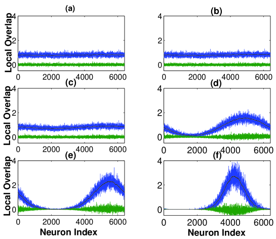
Figure 2: The dependence of the local overlap on $\sigma$. Results are from simulating a network with $N=6400$, $C=320$, $p=32$, $g=0.7$, $a=0.2$ and $\sigma=1900$ (a), $\sigma=1700$ (b), $\sigma=1500$ (c), $\sigma=1000$ (d), $\sigma=700$ (e) and $\sigma=500$ (f). In each panel, the upper fluctuating curve is the local overlap with the retrieved pattern and the lower one the local overlap with one of the non retrieved patterns. The black line inside the local overlap with the retrieved pattern is a smooth version of the local overlap, calculated by averaging over 100 nearby units for each point. A smooth change of the local overlap from a uniform shape to the first Fourier mode is clear.

The simulations indicate that close to the transition the spatial dependence of the overlap takes the form of a cosine, whereas for lower $\sigma$ values it approaches a gaussian. One can easily check analytically, however, that considering a gaussian ansatz for $m_{i}$, and another gaussian for, say, $\rho_{i}$, does not solve the mean-field equations, Eqs.13, which do not in fact appear to admit any simple curve as a solution. This led us to develop approximate treatments that circumvent the lack of a closed-form spatially-dependent solution.

From what we see in the simulations we assume that the transition to the spatially non-uniform solution is smooth (second order). We further assume that $C/\sigma_{c}$ is small so that to a first approximation, in order to determine the critical point, we can neglect the effect of loops, i.e. of $\psi$ and $\Gamma$. This assumption may well be inappropriate (for small $g$, for instance, as we shall see later) but we hypothesize that its effect will not distort a qualitative picture of the phenomenon too much. This can be verified by simulations. Using this ansatz, we now write the solutions of the fixed point equations as follows:

$$m_{i} = m^{0}+\delta m_{i},\hskip 19.91684pt\mid\delta m_{i}\mid\ll m^{0}$$

$$\rho_{i} = \rho^{0}+\delta\rho_{i},\hskip 28.45274pt\mid\delta\rho_{i}\mid\ll\rho^{0}$$

$$T = T^{0}+\delta T\hskip 28.45274pt\mid\delta T\mid\ll T^{0}$$

where $m^{0}$ and $\rho^{0}$ are the uniform parts of the solutions, which we take to be the solutions of the fixed point equations for $\sigma=\infty$; and $\delta m_{i}$ and $\delta\rho_{i}$ are the small deviations from uniformity. In the same way $T^{0}$ is the value of the threshold which sets the mean activity $x=a$ for the uniform solution and $T^{0}+\delta T$ is the (uniform) threshold necessary to keep $x=a$ in the presence of non-uniform terms $\delta m_{i}$ and $\delta\rho_{i}$. It is worth noting that a more accurate approach would be to use the values of $m^{0}$ and $\rho^{0}$ calculated for $\sigma$ just above the transition value $\sigma_{c}$. These values would be different from those at $\sigma=\infty$, as the effects of loops may become important close to the transition to non-uniform solutions; but as stated before we provisionally neglect this inaccuracy. Using these assumptions and expanding the mean-field equation around the uniform solutions one obtains equations for the fluctuations. These equations in the continuum limit are of the following form:

$$\delta m\left(r\right) = \int dr^{\prime}\{\left(\frac{a_{11}}{C}c\left(r,r^{\prime}\right)-\frac{b_{11}}{N}\right)\delta m\left(r^{\prime}\right)+\left(\frac{a_{12}}{C}c\left(r,r^{\prime}\right)-\frac{b_{12}}{N}\right)\delta\rho\left(r^{\prime}\right)\}$$ (21)

$$\delta\rho\left(r\right) = \int dr^{\prime}\{\left(\frac{a_{21}}{C}c\left(r,r^{\prime}\right)-\frac{b_{21}}{N}\right)\delta m\left(r^{\prime}\right)+\left(\frac{a_{22}}{C}c\left(r,r^{\prime}\right)-\frac{b_{22}}{N}\right)\delta\rho\left(r^{\prime}\right)\}$$ (22)

where the coefficients are defined in Appendix III.

Next we take the Fourier transform of the two sides of the above equations, to get:

$$\left(\begin{array}[]{ccc}1-a_{11}e^{-\frac{k^{2}\sigma^{2}}{2}}+b_{21}\frac{\delta(k)}{N}&a_{12}e^{-\frac{k^{2}\sigma^{2}}{2}}-b_{12}\frac{\delta(k)}{N}\\ a_{21}e^{-\frac{k^{2}\sigma^{2}}{2}}-b_{21}\frac{\delta(k)}{N}&1-a_{22}e^{-\frac{k^{2}\sigma^{2}}{2}}+b_{22}\frac{\delta(k)}{N}\end{array}\right)\left(\begin{array}[]{ccc}\delta\tilde{m}\left(k\right)\\ \delta\tilde{\rho}\left(k\right)\end{array}\right)=0.$$

The above equations for $\delta m$ and $\delta\rho$ have a non-trivial solution if and only if the determinant of the matrix of coefficients becomes zero. For $k=0$ the matrix (which includes the $b$ terms) is the same as that which determines the stability of the uniform solution in the network without geometry. On the other hand, when $k\neq 0$ the matrix does not include the $b$ terms, and the vanishing of its determinant yields the critical value of $\sigma$, as it signals the instability of the uniform solution towards the appearance of a non-uniform Fourier mode. For large $\sigma$, the determinant of the coefficient matrix approaches 1, and it decreases with decreasing $\sigma$. For those values of the other parameters (besides $\sigma$) for which the determinant of the matrix is negative at $\sigma=0$, there would be a critical value for $\sigma$ at which the determinant becomes zero, and therefore a transition occurs. It is clear that the first Fourier mode i.e. $k=\frac{2\pi}{N}$ is the one that appears first. This is what one actually observes in simulations.

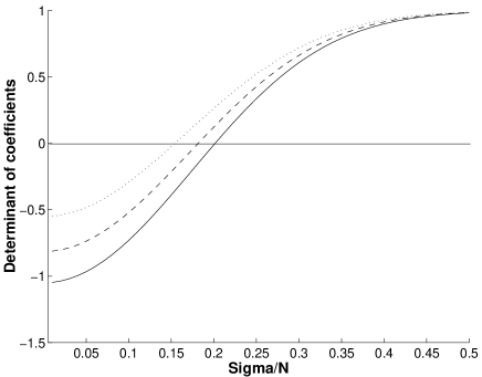
Figure 3: The determinant of the coefficients versus the $\sigma/N$ for $g=0.7$ (full curve), $g=0.6$ (dashed curve) and $g=0.5$ (dotted curve). The other parameters are $a=0.2$ and $p/C=0.1$.

In Fig.3 (full line) we have plotted the determinant of the coefficient matrix as a function of $\sigma/N$ for the first Fourier mode. This is done for three values of $g=0.7,0.6$ and $0.5$. We deduce from this graph that the value of $\sigma_{c}$ increases by increasing $g$. Note however that the first Fourier mode, a cosine, is not strictly speaking a solution of Eqs.13 for any $\sigma$ value below $\sigma_{c}$. The discrepancy becomes more evident, see Fig.2, as $\sigma$ decreases, and the solution eventually becomes localized, i.e. it takes non-zero values for the order parameters only on a limited fraction of the ring. In that regime solutions look like gaussian curves, but they are not exact gaussians.

It is important to realize that the $b$ terms in the above equations come from the effective threshold which results from our uniform inhibitory term, and fixes the mean activity of the network at $x=a$. This is important because if there were no $b$ terms, the condition for the instability of the uniform solution for the non-geometric network and the condition for the appearance of the non-uniform solutions at finite $\sigma$ would have been the same. Therefore without an activity-dependent threshold, stable retrieval in the non-geometric network would have implied no spatially non-uniform solution in its geometric counterpart.

4.2 Storage capacity

The storage capacity of the geometric network differs from that of the non-geometric one for two main reasons. The first one is that by changing the geometry of the connectivity one changes the distribution of the connectivity loops that contribute to noise reverberation in the network. Effectively, lowering $\sigma$ increases the clustering of the nodes in the network [38] and the number of its loops, leading to a decrease in storage capacity for the same reason that the capacity decreases (if expressed as $\alpha\equiv p/C$) when a diluted non-geometric network reaches a denser connectivity.

The second one is the non-uniformity of the spatial distribution of the signal and noise to the units i.e. the spatial dependence of $m(r)$ and $\rho(r)$. Effectively, the connections originating from the less active units at the flanks of the spatial profile are used less, or even unused if the solution is localized and those units remain inactive, and the network becomes roughly equivalent to one with a lower $C$ value.

These two effects are correlated with each other, but one can get an estimate of how they affect the storage capacity by first considering them separately. In other words, one can consider a network with structured connectivity and calculate its storage capacity if the profile of activity has no spatial dependence. Although we know from the previous sections that this kind of uniform solution would not be the stable state of the network, we can calculate this way the effect of the change in the distribution of the loops on the storage capacity. On the other hand, one can consider a network without geometric connectivity, but with a spatially non-uniform activity, although again this would not be the stable solution. We will follow this approach in the coming subsections.

4.2.1 The effect of the loops

We start by considering a uniform solution to the mean-field equations Eqs.13, while considering a gaussian connectivity. The uniform solution is of course not stable nor relevant when $\sigma<\sigma_{c}$: as discussed previously (see Fig.2 and section 4.1) the actual form of the activity is quite close to a cosine immediately below the $\sigma_{c}$; and then slowly transforms to a localized quasi-gaussian activity (Fig2.f) by decreasing $\sigma$. Although we know that the uniform solution is not stable below $\sigma_{c}$, we can still calculate a reference storage capacity by inserting it into the mean-field equations. Then we can compare the results with the simulations and assess their correspondence. In the next section we shall see that this procedure, even though very crude, gives us an estimate of the true storage capacity which is comparable with the simulations.

By considering the uniform solution to the equations, we have:

$$\psi(r-r^{\prime})=\frac{C}{\sqrt{2\pi\sigma^{2}}}\sum_{n=1}^{\infty}e^{-\frac{(r-r^{\prime})}{2(n+1)\sigma^{2}}}\frac{1}{\sqrt{n+1}}\Omega^{n}$$ (23)

and hence:

$$\int dr^{\prime\prime}\{2c(r-r^{\prime\prime})\psi(r-r^{\prime\prime})+\psi(r-r^{\prime\prime})^{2}\}=\frac{C}{\sqrt{2\pi\sigma^{2}}}\sum_{n=1}^{\infty}\frac{n+1}{\sqrt{n+2}}\Omega^{n}$$ (24)

Using the above, we can write the equation for the storage capacity as:

$$A_{2}-\left(1+\frac{C}{\sqrt{2\pi\sigma^{2}}}\sum_{n=1}^{\infty}\frac{n+1}{\sqrt{n+2}}\Omega^{n}\right)\alpha A_{3}=0$$ (25)

Using this equation and evaluating the series numerically, we have calculated the storage capacity for various values of $\sigma$ in a network of $C=320$ and $a=0.2$, as shown in Fig.6. This graph indicates that the storage capacity decreases with $\sigma$ but not by much. The assumption of considering the uniform solution implies that such a decrease is due solely to the increased relevance, as $\sigma$ decreases, of closed loops, and therefore of increased noise reverberation. Although this analysis does not take into account additional effects due to the emergence of non-uniform solutions, we shall see in the next section that the capacity decrease in the graph is quite comparable with the results of the simulations, also for values of $\sigma$ which lead to non-uniform steady states.

4.2.2 The effect of the non-uniform solution

We can have an idea of how the form of the solution affects the storage capacity simply by considering an ansatz on the form of $\rho(r)$ and $m(r)$ which depends on a finite set of parameters $\{\lambda_{1},\lambda_{2},\cdots,\lambda_{k}\}$. We also assume, to start with, that the effects of loops are negligible, so that we can set $\psi(r,r^{\prime})=0$ and $\Gamma(r)=0$. Loops are of course not negligible e.g. when $\sigma$ is small, but we want now to isolate the effect of the non-uniformity from that of loops, which has been estimated in the previous part using the uniform solution. In other words by this procedure we actually consider a network without loops and calculate the storage capacity corresponding to a parametrized non-uniform activity profile, although we know it is unstable in a structure-less network.

With this ansatz and integrating over $r$ on both the left and right hand sides of the equations describing $\rho(r)$ and $m(r)$, i.e. Eqs.13, we can write after some manipulation:

$$\left(\frac{\int drI_{2}(r)}{T_{0}\int drm(r)}\right)^{2} - \alpha\frac{\int drI_{3}(r)}{\int dr[\rho(r)]^{2}}=0$$ (26)

$$x = \frac{\int drm(r)}{\int drI_{2}(r)}\int drI_{4}(r)$$ (27)

$$I_{2}(r) = \langle(\frac{\eta(r)}{a}-1)\int^{+}Dz((\frac{\eta(r)}{a}-1)m(r)+b(x)-T_{thr}-\rho(r)z)\rangle$$

$$I_{3}(r) = \langle\int^{+}Dz((\frac{\eta(r)}{a}-1)m(r)+b(x)-T_{thr}-\rho(r)z)^{2}\rangle$$

$$I_{4}(r) = \langle\int^{+}Dz((\frac{\eta(r)}{a}-1)m(r)+b(x)-T_{thr}-\rho(r)z)\rangle$$

In practice, for any given form of the functions $m(r)$ and $\rho(r)$, one can solve Eq.27 to get $b(x)-T_{thr}$ by setting its r.h.s to $x=a$. Then one can use this to evaluate the integrals appearing in Eq.26 and find the highest value of $\alpha$ for which a solution for this equation exists in the $\{\lambda_{1},\lambda_{2},\cdots,\lambda_{k}\}$ space.

As an example, let us consider a gaussian form, which simulations indicate is a reasonable approximation, even if not an exact solution, in the localized, or low $\sigma$, regime. In other words, let us assume that $m(r)=m_{0}exp(-r^{2}/2l^{2})$ and $\rho(r)=\rho_{0}exp(-r^{2}/2l^{2})$. By fixing $l$ and following the procedure described above one finds that for a given value of $\alpha$, Eq.26 appears as a closed curve in the $(m_{0},\rho_{0})$ plane, that shrinks in size with increasing $\alpha$, analogously to Eq.18. The value of $\alpha$ for which this closed curve disappears defines the storage capacity at constant width $\alpha(l)$. Of course the gaussian ansatz is an approximation which needs to be considered carefully. An example of gaussian-like activity is Fig.2.f. Unfortunately the profile of activity below $\sigma_{c}$ does not take an analytical form. Still, a gaussian fit seems to be a good approximation, even though it is not the solution (note that in Fig.2.f the activity goes to zero outside a finite radius, hence it cannot be a gaussain). The accuracy of the gaussian ansatz can be checked by comparing the resulting storage capacity with that of the simulations. As we shall discuss in the next section, our procedure leads to a reasonable agreement with the simulations.

Fig.4 shows the result of following the above procedure for calculating $\alpha(l)$ for a network of $N$ units and $a=0.2$. The decrease in the storage capacity for more localized solutions can be seen. This decrease is solely due to the non-uniformity of the solution, and it has no contribution from the geometry of the connectivity, since the effect of the connectivity decouples when one integrates over space in the mean-field equations to get Eq.26. In other words, there is no dependence on the connectivity probability distribution $c(r,r^{\prime})$ in this equation.

Figure 4: The dependence of the storage capacity, for $a=0.2$, on $l/N$, where $l$ is the width of a gaussian solution. Note the correspondence with the $\sigma$ values used in Fig.2: see text.

In Fig.4 we have indicated, on the $l/N$ axis, the widths of the profiles seen in the simulations with the 6 values of $\sigma$ used in Fig.2. We have run extensive simulations with those 6 values of $\sigma$ but, unlike those in Fig.2, with $\alpha$ close to $\alpha_{c}$ and $g$ to the optimal gain value, as estimated from the simulations themselves. To calculate the values of $l$ corresponding to each $\sigma$ and close to capacity we have used equation Eq. 29: we first calculate the average value of $q$ across simulations with each $\sigma$, by using its definition Eq.28, and then find the value $l$ which solves Eq.29. Please note that the gaussian fit is a reaonable approximation, only in the localized regime e.g. Fig.2e and f, but not really for apparently flat solutions like those in Fig.2a or even cosine-like ones like those in Fig.2c. Moreover, finite size effects smooth the otherwise sharp transition at $\sigma_{c}$. Finally, Fig.2 was produced by running simulations at low $\alpha$ and fixed $g$, whereas we now set these parameters at the storage capacity limit. All these effects cumulate to make the estimated $l$ values smaller than what one would have predicted from visually inspecting Fig.2a-c (the discrepancy is milder in the localized regime). For example, looking at point $a$ in Fig.4 one sees $l=1.4N$ for $\sigma=1900$, while from the flat-looking solution of Fig.2 one might have expected $l\to\infty$!

One can see that such widths change significantly, and correspondingly there is a significant estimated capacity decrease, for the upper 3 $\sigma$ values, which are relatively clustered around $\sigma_{c}$. For the lower 3 $\sigma$ values, even though they cover a much larger range on a log scale, the resulting profile widths change less ($l$ is roughly proportional to $\sigma$), as the solutions have become effectively localized. Correspondingly, the storage capacity does not decrease further due the profiles of the solutions, although it continues to decrease due to more clustered connectivity. The second of the two mechanisms which decrease the storage capacity thus reaches a maximum effect as soon as the two flanks of the activity profile go to zero, and the steady state of the network is a genuine ’bump’.

5 Simulations

In this section we present the results of simulations that investigate the relation between the storage capacity and the width of the connectivity, as well as the emergence of non-uniform asymptotic states. Such states for very local connectivity (very low $\sigma$) eventually become localized, in the sense that activity is zero outside a limited fraction of the ring.

To measure the degree of uniformity of the steady states reached in each simulation, we define the quantity:

$$q=\frac{12\int dr\left(r-r_{max}\right)^{2}m\left(r\right)}{N^{2}\int drm\left(r\right)}$$ (28)

where $r_{max}$ is where the local overlap $m\left(r\right)$ has its maximum. We use a smoothed version of the local overlap to regularize the parameter $0<q\leq 1$, which takes its maximum $q=1$ for a uniform solution and is inversely related to the degree of bumpiness, or of locality, of a spatially non-uniform overlap distribution [5].

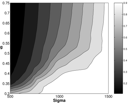
Figure 5: The change in the uniformity $q$ as a function of $g$ and $\sigma$ from simulating a network of $N=6400$, $C=320$. The sparsity of the patterns is $a=0.2$. The value of $p$ is chosen in a way that the network on average is able to retrieve $50\%$ of the patterns for the given values of $g$ and $\sigma$.

Here we report the results of simulating a network composed of $N=6400$ units with $C=320$ and $a=0.2$. For each value of $\sigma$, $g$ and $p$ we give the network a full cue, corresponding to one of the stored patterns, and after $50$ synchronous updates we measure the final overlap with the presented pattern. If the final overlap is larger than $0.4$ we take it to be a successful retrieval. We repeat this for $4$ different seeds for the random number generator and $5$ different patterns and then index the performance of the network with the percent of patterns retrieved (according to the above criteria). We take the value of $p$ at which the performance reaches $50\%$ as a measure of the storage capacity for those values of $g$ and $\sigma$. By repeating for different values of $g$ we thus assess the optimal storage capacity for the network, optimized across values of the gain.

In Fig.5 one can observe the way $q$ changes as a function of $g$ and $\sigma$. As we found in section 4, for values of $\sigma$ below the transition the activity is not uniform in space, i.e. it has a ’bumpy’ profile. Increasing $g$ favours the localization of the solution, which for high $g$ and low $\sigma$ becomes a genuine ’bump’ of activity, as seen in Fig.2. There appears to be no sharp transition, but rather a very smooth cross-over, from the ’quasi-cosine’ regime near $\sigma_{c}$ to the localized ’quasi-gaussian’ regime for low $\sigma$. The cross-over is in fact regulated by the gain $g$.

The second point that we have studied through the simulations is the dependence of the storage capacity on the width of the connectivity $\sigma$. The storage capacity calculated from the simulations is the full curve in Fig.6. This curve lies below the storage capacity calculated analytically using the uniform solution. As previously mentioned there are two effects which contribute to the decrease of the storage capacity. First, the increase in the number of loops as a result of the decrease in the width of the connectivity, which has the effect discussed in section 4.2.1 and shown with the dashed curve in Fig.6. Second, the non-uniform profile of the solution, discussed in section 4.2.2. These two effects are not uncorrelated but one can consider them combined as if they were uncorrelated, in the following way. For each value of $\sigma$ one first calculates the storage capacity by considering only the effects of the loops, i.e. the dashed curve. Then one estimates the most appropriate width for a model localized solution, i.e. the best gaussian fit, by solving the following equation for $l$, using the value $q$ obtained from the simulations:

$$q=\frac{12\int_{-0.5}^{0.5}drr^{2}exp(-\frac{r^{2}N^{2}}{2l^{2}})}{\int_{-0.5}^{0.5}drexp(-\frac{r^{2}N^{2}}{2l^{2}})}$$ (29)

Then an estimate of the storage capacity, given independent effects of loops and localization, would simply be the multiplication of the storage capacity calculated for the uniform solution by the factor $\alpha(l)/\alpha(\infty)$. This is the dotted curve in Fig.6. It yields a lower estimate of the storage capacity as compared to that of the simulations, but yet closer to it than the uniform solution approximation. The assumption of uncorrelated effects thus overestimates the capacity decrease with lower $\sigma$ values.

Note that the capacity decrease could in principle be overestimated also as an effect of our procedure of exploring only spatially-dependent solutions of a given shape (in particular, gaussian); this effect is however likely negligible, at least in the localized regime where the profiles seen in the simulations are very close to gaussian.

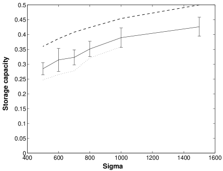
Figure 6: In this graph, the full curve shows the storage capacity versus $\sigma$ for $a=0.2$, obtained numerically simulating a network with $N=6400$, $C=320$. The dashed curve is the storage capacity estimated analytically using the uniform approximation, as discussed in section 4.2.1. The dotted line represents the storage capacity estimated taking into account, as uncorrelated, both the effect of more loops and that of the spatial dependence of the solution, as explained in section 4.2.2.

6 Discussion

In this paper we have studied the retrieval properties of an autoassociative network with geometric synaptic connectivity. To approach the analysis of a spatially structured network we had to find alternatives to the standard thermodynamic formalism often applied to systems with quenched disorder, based on the calculation of a free-energy with the replica trick, and on its evaluation at a saddle point. Even though in terms of their behaviour and even of their fixed point equations asymmetric and symmetric networks do not differ by much at least in networks with threshold-linear units for which the spin glass phase is irrelevant [35], the lack of a Hamiltonian requires an alternative approach to obtain the mean-field equations. Fukai and Shiino developed years ago a ’self-consistent signal-to-noise analysis’ to treat cases in which a Hamiltonian could not be defined, in particular asymmetric networks [26] and networks with arbitrary analogue transfer functions [27]. The asymmetric connectivity is in some sense a technical problem, which might not reveal any ’new’ physics in the threshold-linear networks. In our case, we had to face a second and more substantive problem, as a direct result of the geometry in the connectivity. This is the fact that in order to describe the behavior of a geometric network, one needs to introduce order parameters that are not scalars but scalar fields. This makes the derivation of the mean-field equations and the analysis of their solutions much more challenging: the equations are now integral equations in these field order parameters (see Eq.13). We adapted the ’self-consistent signal-to-noise analysis’ turning it into a local signal-to-noise approach, to find self-consistent equations for order parameters with the following physical meaning:

• $m(r)$: the local overlap, i.e. the product of the current activity and the stored patterns, summed over all units presynaptic to the unit at $r$.

• $\rho(r)$: the local noise, i.e. the mean square amplitude of the non-condensed overlaps [3], as seen at $r$.

• $\psi(r,r^{\prime})$: the effect of the direct and indirect connections linking two units at positions $r$ and $r^{\prime}$ on the reverberation of the noise.

• $\Gamma(r)$: a measure, proportional to the diagonal elements of $\psi(r,r^{\prime})$, of the effect of the activity of each unit on the noise component of its own input.

Although the stored patterns do not include any spatial structure or correlation, the retrieval states of the geometric connectivity network, as simulations easily demonstrate, may have non-uniform activity profiles when the connections are short range enough. The activity profile of the retrieval state can even become localized in space, as a ’bump’ of activity, in the appropriate parameter regime. It is worth emphasizing that a non-uniform retrieval state does not correspond in full to the stored pattern that is being retrieved, since the stored pattern does not have any spatial preference; the retrieval state has a large overlap with the pattern, but circumscribed to the bump. As shown in Fig.5, the bumpiness of such a non-uniform retrieval state depends not only on how short range is the connectivity, but also on the gain of the input-output transfer function. Increasing the gain favours localization in the retrieval state, of course as long as the network remains in the regime where retrieval occurs.

Given that the storage capacity of the geometric network decreases with respect to that of a uniform network due to both an increase in the loops and the non-uniformity of the solution, we described a procedure to estimate these effects under the assumption that they are independent. Comparing with simulations, we found that the procedure yields a reasonable estimate of the storage capacity, although lower than the true value, due probably to the simplifying independence assumption. The bottom-line conclusion is that as the connectivity of the autoassociative network becomes shorter range, its storage capacity, expressed as $p/C$, decreases indeed, but not by a large factor.

The model that we have studied here is defined on a ring, i.e. it is a one dimensional model. Although we do not expect significant differences between the results reported here and those of a more interesting model in two dimensions, it remains to be checked, in future work, to what extent the results can be generalized to a 2D model.

Further, we have considered a gaussian connectivity of varying width. An alternative model, introduced by Watts and Strogatz [38], is that of a network with a fraction of connections strictly short range, and the complementary fraction distributed at random across the entire network. This could be perhaps an appropriate model for cortical connectivity, with its short- and long-range connections [8], and it has already been considered, albeit in a geometry-free formulation, as a model of semantic memory [22, 14]. It seems important to be able to extend our approach to a model of the Watts-Strogatz type, with 1D or 2D geometry. It is possible that the storage capacity would decrease more substantially in such a model, than it does in the one considered here - a naive expectation is that $p$ should scale, essentially, with the number of short range connections, those that comprise the so-called regular network.

Indeed, the Watts-Strogatz autoassociative model has been studied by [5], even though with simulations only and a more realistic neuronal integrate-and-fire dynamics. One result of that study is the near incompatibility between localization and retrieval, which appear to occur in almost mutually exclusive ranges of the relevant parameter, the fraction of short-range connections. The fact that retrieval did not seem to succeed when asymptotic firing states are localized may have been due to a strongly decreased capacity, or to instabilities associated with the integrate-and-fire dynamics, or to other aspects of that model, such as the mechanism implementing inhibitory control of the activity of excitatory units. Whatever the case, this emphasizes the need for studies of associative retrieval and localization in realistic neural network models. Important features that need consideration are the dynamics of individual units and the model adopted for inhibitory effects.

Once thus extended, this approach has the potential to yield a quantitative assessment of the storage capacity of cortical modules in the mammalian brain. Such modules obviously differ from our simplified mathematical models in several respects, but an educated guess predicts that the crucial factor that determines their storage capacity is the number and geometrical distribution of the Hebbian-modifiable connections that the average unit receives.

It becomes possible at that stage to consider in a realistic setting a phenomenon which had been considered earlier in rather abstract models: the coexistence of multiple retrieval states. So-called ’spurious’ solutions have been shown not to be stable, essentially, in threshold-linear networks without geometry [24], but in a simple ring model [21] different stored patterns can be retrieved in different portions of the ring. Thus the underlying geometrical manifold can turn spurious mixtures of patterns into interesting combinations of localized patterns, and this raises the issue of their competitive interactions. Recent neurophysiological work [23] demonstrates that the receptive fields of visually evoked activity patterns are effectively restricted 2- to 3-fold, in the macaque temporal cortex, when several objects are present together in the visual scene. This finding may have a correlate in an associative memory network with geometry, where long-range inhibition may restrict the width of activity profiles retrieved on different portions of the manifold.

Appendix.I

Using Eq.12, the solution for $m^{\mu}_{i}$ can be written as:

$$m_{i}^{\mu}=\frac{1}{C}R^{\mu}_{ii}(\eta_{i}^{\mu}/a-1)G^{\mu}[i]+\frac{1}{C}\sum_{j\neq i}R^{\mu}_{ij}(\eta_{j}^{\mu}/a-1)G^{\mu}[j]$$ (I-1)

where $R_{ij}^{\mu}$ is expanded in a power series as:

$$R_{ij}^{\mu}=c_{ij}+\sum_{l}K_{il}^{\mu}c_{lj}+\sum_{lt}K_{il}^{\mu}K_{lt}^{\mu}c_{tj}+\ldots$$ (I-2)

and we have used the notation $G^{\mu}[i]=G[(\eta_{i}^{1}/a-1)m_{i}^{1}+\rho_{i}^{\mu}z+b(x)-T_{thr}]$.

Now that we have expressed the local overlap with a non-retrieved pattern as a function of $m^{1}_{i}$, we can proceed to evaluate $\rho$ and $\gamma$:

$$\sum_{\nu\neq 1}(\eta_{i}^{\nu}-1)m_{i}^{\nu} = \frac{1}{C}\sum_{\nu\neq 1}R_{ii}^{\nu}(\eta_{i}^{\nu}/a-1)^{2}G^{\nu}[i]$$

$$+ \frac{1}{C}\sum_{j\neq i,\nu\neq 1}R_{ij}^{\nu}(\eta_{i}^{\nu}/a-1)(\eta_{j}^{\nu}/a-1)G^{\nu}[j].$$

For the first sum in the r.h.s of Eq.Appendix.I above, using the independence of different patterns and assuming that $\rho_{i}^{\mu}\simeq\rho_{i}$ one can write:

$$\frac{1}{C}\sum_{\nu\neq 1}R_{ii}^{\nu}(\eta_{i}^{\nu}/a-1)^{2}G^{\nu}[i] = \alpha\langle R_{ii}^{\nu}(\eta_{i}^{\nu}/a-1)^{2}G^{\nu}[i]\rangle$$

$$\simeq \alpha\langle R_{ii}^{\nu}(\eta_{i}^{\nu}/a-1)^{2}\rangle v_{i}$$

and as a result we identify:

$$\gamma_{i}=\alpha<R_{ii}^{\nu}(\eta_{i}^{\nu}/a-1)^{2}>=\alpha T_{0}\langle R_{ii}^{\nu}\rangle,$$ (I-5)

where we denote as in [32] $T_{0}\equiv 1/a-1$; and therefore:

$$\Gamma_{i}=\alpha T_{0}(\langle R_{ii}^{\nu}\rangle-c_{ii})=\alpha T_{0}\langle\sum_{l}K_{il}^{\mu}c_{lj}+\sum_{lt}K_{il}^{\mu}K_{lt}^{\mu}c_{tj}+\dots\rangle.$$ (I-6)

The second term is a bit tricky. For this term, by replacing the sum with the average we get zero mean, but for the standard deviation we have:

$$\rho^{2}=\frac{\alpha}{C}(1/a-1)\sum_{j}\langle{R_{ij}^{\nu}}^{2}(\eta_{j}^{\nu}/a-1)^{2}G^{\nu}[j]^{2}\rangle$$ (I-7)

which is, actually, the standard deviation of the noise. We can then replace the second term, that is the noise term, with a gaussian random variable with mean zero and standard deviation $\rho$, and take it into account in our mean-field equations by averaging the equations over this gaussian measure. We shall discuss the reliability of this assumption soon.

In order to make the equations more comprehensive, we define the order parameter $\psi$ as an average over non-retrieved patterns of $\psi^{\mu}$, where:

$$\psi_{ij}^{\mu}=R^{\mu}_{ij}-c_{ij}=\sum_{l}K_{il}^{\mu}c_{lj}+\sum_{lt}K_{il}^{\mu}K_{lt}^{\mu}c_{tj}+\ldots$$ (I-8)

By using this definition with some algebraic manipulation we get the mean-field equations.

Considering the noise term as a gaussian random variable comes from rewriting the left hand side of Eq.7 in its original form and then approximating it as a sum of random independent variables:

$$\rho_{i}z+\gamma_{i}v_{i}=\frac{1}{C}\sum_{\nu\neq 1,j}c_{ij}(\eta_{i}^{\nu}/a-1)(\eta_{j}^{\nu}/a-1)v_{j}$$ (I-9)

The assumption of independence of these terms is a bit tricky, since in general when following the dynamics of the system the activity of each unit $v_{i}$ at a given time depends on the local field at the previous time step, hence on the patterns. However, it becomes an appropriate approximation when the first pattern is thoroughly retrieved i.e. $v_{i}=\eta_{i}^{1}$. In this case the terms that appear in the noise sum are in fact close to independent random variables, as the patterns are, by construction. The gaussian noise assumption is thus accurate in the limit in which the solutions of the mean-field equations are exactly equal to the patterns used in generating the weight matrix, i.e. in the case of retrieval without errors. This is of course never strictly the case, unless the storage capacity is zero in the thermodynamic limit[1]. However, if we assume that the retrieved state in a successful retrieval is very close to a stored pattern and has a large overlap with it, then the gaussian approximation is reasonable. In other words the gaussian noise is appropriate when retrieval really occurs.

It is important to note that one should be careful in using the gaussian approximation when dealing with the dynamics of the network. This approximation may just qualitatively predict the recall dynamics when retrieval occurs (as well as the stationary state phase diagram) but it fails to describe the non-retrieval trajectories. This is simply due to the fact that the noise distribution can be approximated by a gaussian when retrieval is successful, as explained above, but it could be non-gaussian in the intermediate states before getting close to the retrieval attractor. Starting from an initial state which for instance has a non-zero overlap with two patterns, the noise does not follow in general a gaussian distribution. It approaches a gaussian form as the network evolves toward one of the attractors, corresponding to one of the patterns. The gaussian approximation may also give the correct dynamical equations for the fist few time steps, but then it may give results different from the exact solutions later on. For a detailed discussion on this issue see [11, 9].

As we shall see later in the limit of a structure-less network the mean-field equations from the gaussian approximation are identical to those found previously using the replica method. This confirms that the equations that result from the gaussian approximation in the signal-to-noise analysis are in terms of accuracy in the same line as the equations derived with the replica method. Actually the close relation between the signal-to-noise analysis, the replica method and the TAP equation has been investigated in a recent paper by Shiino and Yamana [28].

Appendix.II

Dividing by the gain factor the equations for $\rho$ and $m$ one gets:

$$\left(\frac{gT_{0}}{1-g\Gamma}\right)^{-2} = \alpha\left(1+2\psi+\frac{N}{C}\psi^{2}\right)A_{3}$$

$$\left(\frac{gT_{0}}{1-g\Gamma}\right)^{-1} = A_{2}$$

On the other hand using the equation for $\psi$ and the definition of $\Omega$ in Eq.14 we have:

$$2\psi+\frac{N}{C}\psi^{2} = \frac{C}{N}\frac{(2-\Omega)\Omega}{(1-\Omega)^{2}}$$

and we find:

$$\Omega=\langle\int^{+}Dz\rangle/A_{2}.$$

Combining the equations above one gets to Eqs.18 and 19. The second of those equations determines the optimal value of $g$, but it does not change the storage capacity.

Appendix.III

$$a_{11} = g\langle\left(\frac{\eta}{a}-1\right)^{2}\phi\left(w+v\eta/a\right)\rangle$$

$$b_{11} = g\langle\left(\frac{\eta}{a}-1\right)\phi\left(w+v\eta/a\right)\rangle^{2}/\Delta$$

$$a_{12} = g\langle\left(\frac{\eta}{a}-1\right)\beta\left(w+v\eta/a\right)\rangle$$

$$b_{12} = g\langle\left(\frac{\eta}{a}-1\right)\phi\left(w+v\eta/a\right)\rangle\langle\beta\left(w+v\eta/a\right)\rangle/\Delta$$

$$a_{21} = \alpha g^{2}T_{0}^{2}\langle(\frac{\eta}{a}-1)\left((w+v\eta/a)\phi\left(w+v\eta/a\right)+\beta\left(w+v\eta/a\right)\right)\rangle$$

$$b_{12} = \alpha g^{2}T_{0}^{2}\langle\left((w+v\eta/a)\phi\left(w+v\eta/a\right)+\beta\left(w+v\eta/a\right)\right)\rangle\langle\left(\frac{\eta}{a}-1\right)\phi\left(w+v\eta/a\right)\rangle/\Delta$$

$$a_{22} = \alpha g^{2}T_{0}^{2}\langle\phi\left(w+v\eta/a\right)\rangle$$

$$b_{22} = \alpha g^{2}T_{0}^{2}\langle\left((w+v\eta/a)\phi\left(w+v\eta/a\right)+\beta\left(w+v\eta/a\right)\right)\rangle\langle\beta\left(w+v\eta/a\right)\rangle/\Delta$$

$$\Delta = \langle\phi\left(w+v\eta/a\right)\rangle$$

$$\phi\left(x\right) = \frac{1}{\sqrt{2\pi\sigma^{2}}}\int_{-\infty}^{x}dz\exp(-z^{2}/2)$$

$$\beta\left(x\right) = \frac{1}{\sqrt{2\pi\sigma^{2}}}\exp(-x^{2}/2).$$

where we have set $r=m_{0}/\rho_{0}$ and $w=[b\left(x\right)-m_{0}-T_{thr}]/\rho_{0}$.

References

- [1] Amari S and Maginu K, Statistical neurodynamics of associative memory, 1988 Neural Networks 1 63
- [2] Amaral DG and Witter MP, The three-dimensional organization of the hippocampal formation: a review of anatomical data, 1989 Neuroscience 31 571
- [3] Amit DJ, Modelling Brain Function, 1989 (Cambridge Univ. Press, New York).
- [4] Amit DJ and Tsodyks MV, Quantitative study of attractor neural network retrieving at low spike rates: I. Substrates – spikes, rates and neuronal gain, 1991 Network: Comput. Neural Syst. 2 259
- [5] Anishchenko A, Bienenstock E and Treves A, Autoassociative Memory Retrieval and Spontaneous Activity Bumps in Small-World Networks of Integrate-and-Fire Neurons, 2004 SISSA preprint
- [6] Battaglia FP and Treves A, Attractor neural networks storing multiple space representations: A model for hippocampal place, 1998 Phys. Rev. E 58 7738
- [7] Ben-Yishai R, Bar-Or RL and Sompolinsky H, Theory of orientation tuning in visual cortex, 1995 Proc. Natl. Acad. Sci. USA 92 3844
- [8] Braitenberg V and Schuz A (1991) Anatomy of the Cortex (Springer-Verlag, Berlin).
- [9] Bolle D, Busquets Blanco J and Verbeiren T, The signal-to-noise analysis of the Little-Hopfield model revisited, cond-mat/0307499
- [10] Buonomano DV and Merzenich MM, Cortical plasticity: From synapses to maps, 1998 Annu. Rev. Neurosci. 21 149
- [11] Coolen A C C, Statistical mechanics of recurrent networks II: Dynamics, cond-mat/0006011
- [12] Derrida B, Gardner E and Zippelius A, An exactly solvable asymmetric neural network model, 1987 Europhys. Lett. 4 167.
- [13] Felleman DJ and Van Essen DC, Distributed hierarchical processing in the primate cerebral cortex, 1991 Cereb. Cortex 1 1.
- [14] Fulvi Mari C and Treves A, Modeling neocortical areas with a modular neural network, 1998 Biosystems 48 47
- [15] Hellwig B, A quantitative analysis of the local connectivity between pyramidal neurons in layers 2/3 of the rat visual cortex, 2000 Biol. Cyber. 82 111
- [16] Hopfield JJ, Neural networks and physical systems with emergent collective computational abilities, 1982 Proc. Natl. Aca. Sci. USA 79 2554
- [17] Kuhn R, Bos S and Vanhemmen JL, Statistical mechanics for networks of graded response neurons, Phys. Rev. A 1991 43 2084
- [18] Martin SJ and Morris RGM, New life in an old idea: The synaptic plasticity and memory hypothesis revisited, 2002 Hippocampus 12 609
- [19] McNaughton BL and Morris RGM, Hippocampal synaptic enhancement and information storage within a distributed memory system, 1987 Trends Neurosci. 10 408
- [20] Monnason R, Storage of spatially correlated patterns in autoassociative memories,1993 J. Phys. I Paris 3 1141
- [21] Morelli LG, Abramson G and Kupermanet MN, Associative memory on a small-world neural network, 2003 oai:arXiv.org:nlin/0310033
- [22] O’Kane D and Treves A, Why the simplest notion of neocortex as an autoassociative memory would not work, 1992 Network: Comp. Neural Syst. 3 379
- [23] Rolls ET, Aggelopoulos NC and Zheng F, The receptive fields of inferior temporal cortex neurons in natural scenes, 2003 J. Neurosci. 23 339
- [24] Roudi Y and Treves A, Disappearance of spurious states in analog associative memories, 2003 Phys. Rev. E 67:041906
- [25] Samsonovich A and McNaughton BL, Path integration and cognitive mapping in a continuous attractor neural network model, 1997 J. Neurosci. 17 5900
- [26] Shiino M and Fukai T, Self-consistent signal-to-noise analysis and its application to analogue neural network with asymmetric connections, 1992 Jour. of Phys. A: Math. Gen. 25 L375
- [27] Shiino M and Fukai T, Self-consistent signal-to-noise analysis of the statistical behavior of analog neural networks and enhancement of the storage capacity. 1993 Phys. Rev. E 48 867
- [28] Shiino M and Yamana M, Statistical mechanics of stochastic neural networks: Relationship between the self-consistent signal-to-noise analysis, Thouless-Anderson-Palmer equation, and replica symmetric calculation approaches, 2004 Phys. Rev. E 96 011904
- [29] Sompolinsky H, Neural networks with nonlinear synapses and a static noise, 1986 Phys. Rev. A 34 2571
- [30] Squire LR, Memory and the hippocampus: A synthesis from findings with rats, monkeys, and humans, 1992 Psychol. Rev. 99 195
- [31] Touretzky DS, Redish AD, Theory of rodent navigation based on interacting representations of space, 1996 Hippocampus 62 47
- [32] Treves A, Graded-response neurons and information encoding, 1990 Phys. Rev. A 42 2418
- [33] Treves A and Rolls ET, What determines the capacity of autoassociative memories in the brain, 1991 Network: Comp. Neural Syst. 2 371
- [34] Treves A, Dilution and sparse coding in threshold-linear nets, 1991 J. Phys. A: Math. Gen. 24 327
- [35] Treves A, Are spin-glass effects relevant to understanding realistic auto-associative networks?, 1991 Jour. of Phys. A: Math. Gen. 24 2645
- [36] Treves A and Rolls ET, A computational analysis of the role of the hippocampus in memory, 1994 Hippocampus 4 374.
- [37] Tsodyks MV and Feigel’man MV, The enhanced storage capacity in neural networks with low activity level, 1988 Europhys. Lett. 6 101
- [38] Watts DJ and Strogatz SH, Collective dynamics of ’small world ’ networks, 1998 Nature 393 440