The renormalization group approach - from Fermi liquids to quantum dots

1 The RG: what, why and how

Imagine that you have some problem in the form of a partition function

$$Z(a,b)=\int dx\int dye^{-a(x^{2}+y^{2})}e^{-b(x+y)^{4}}$$ (1)

where $a,b$ are the parameters.

First consider $b=0$, the gaussian model. Suppose that you are just interested in $x$, say in its fluctuations. Then you have the option of integrating out $y$ and working with the new partition function

$$Z(a)=N\ \int dxe^{-ax^{2}}$$ (2)

where $N$ comes from doing the $y$-integration. We will ignore such an $x$-independent pre-factor here and elsewhere since it will cancel in any averaging process.

Consider now the nongaussian case with $b\neq 0$. Here we have

$$Z(a^{\prime},b^{\prime}...) = \int dx\left[\int dye^{-a(x^{2}+y^{2})}e^{-b(x+y)^{4}}\right]$$ (3)

$$\equiv \int dxe^{-a^{\prime}\ x^{2}}e^{-b^{\prime}x^{4}-c^{\prime}x^{6}+...}$$

where $a^{\prime}$, $b^{\prime}$ etc., define the parameters of the effective field theory for $x$. These parameters will reproduce exactly the same averages for $x$ as the original ones. This evolution of parameters with the elimination of uninteresting degrees of freedom, is what we mean these days by renormalization, and as such has nothing to do with infinities; you just saw it happen in a problem with just two variables.

The parameters $b$, $c$ etc., are called couplings and the monomials they multiply are called interactions. The $x^{2}$ term is called the kinetic or free-field term.

Notice that to get the effective theory we need to do a nongaussian integral. This can only be done perturbatively. At the simplest tree Level, we simply drop $y$ and find $b^{\prime}=b$. At higher orders, we bring down the nonquadratic exponential and integrate in $y$ term by term and generate effective interactions for $x$. This procedure can be represented by Feynman graphs in which variables in the loop are limited to the ones being eliminated.

Why do we do this? Because certain tendencies of $x$ are not so apparent when $y$ is around, but surface to the top, as we zero in on $x$. For example, we are going to consider a problem in which $x$ stands for low-energy variables and $y$ for high energy variables. Upon integrating out high energy variables a numerically small coupling can grow in size (or initially impressive one diminish into oblivion), as we zoom in on the low energy sector.

This notion can be made more precise as follows. Consider the gaussian model in which we have just $a\neq 0$. We have seen that this value does not change as $y$ is eliminated since $x$ and $y$ do not talk to each other. This is called a fixed point of the RG. Now turn on new couplings or ”interactions” (corresponding to higher powers of $x$, $y$ etc.) with coefficients $b$, $c$ and so on. Let $a^{\prime}$, $b^{\prime}$ etc., be the new couplings after $y$ is eliminated. The mere fact that $b^{\prime}>b$ does not mean $b$ is more important for the physics of $x$. This is because $a^{\prime}$ could also be bigger than $a$. So we rescale $x$ so that the kinetic part, $x^{2}$, has the same coefficient as before. If the quartic term still has a bigger coefficient, (still called $b^{\prime}$), we say it is a relevant interaction. If $b^{\prime}<b$ we say it is irrelevant. This is because in reality $y$ stands for many variables, and as they are eliminated one by one, the coefficient of the quartic term will run to zero. If a coupling neither grows not shrinks it is called marginal.

There is another excellent reason for using the RG, and that is to understand the phenomenon of universality in critical phenomena. I must regretfully pass up the opportunity to explain this and refer you to Professor Michael Fisher’s excellent lecture notes in this very same school many years ago MEF .

We will now see how this method is applied to interacting fermions in $d=2$. Later we will apply these methods to quantum dots.

2 The problem of interacting fermions

Consider a system of nonrelativistic spinless fermions in two space dimensions. The one particle hamiltonian is

$$H={K^{2}\over 2m}-\mu$$ (4)

where the chemical potential $\mu$ is introduced to make sure we have a finite density of particles in the ground state: all levels up the Fermi surface, a circle defined by

$$K^{2}_{F}/2m=\mu$$ (5)

are now occupied and occupying these levels lowers the ground-state energy.

Notice that this system has gapless excitations above the ground state. You can take an electron just below the Fermi surface and move it just above, and this costs as little energy as you please. Such a system will carry a dc current in response to a dc voltage. An important question one asks is if this will be true when interactions are turned on. For example the system could develop a gap and become an insulator. What really happens for the $d=2$ electron gas?

We are going to answer this using the RG. Let us first learn how to do RG for noninteracting fermions. To understand the low energy physics, we take a band of of width $\Lambda$ on either side of the Fermi surface. This is the first great difference between this problem and the usual ones in relativistic field theory and statistical mechanics. Whereas in the latter examples low energy means small momentum, here it means small deviations from the Fermi surface. Whereas in these older problems we zero in on the origin in momentum space, here we zero in on a surface. The low energy region is shown in Figure 1.

Figure 1: The low energy region for nonrelativistic fermions lies within the annulus concentric with the Fermi circle.

To apply our methods we need to cast the problem in the form of a path integral. Following any number of sources, say rmprg we obtain the following expression for the partition function of free fermions:

$$Z_{0}=\int d\psi d\overline{\psi}e^{S_{0}}\\$$ (6)

where

$$S_{0}=\int d^{2}K\int_{-\infty}^{\infty}d\omega\overline{\psi}(\omega,{\mathbf{K}})\left(i\omega-{(K^{2}-K_{F}^{2})\over 2m}\right)\psi(\omega,{\mathbf{K}})$$ (7)

where $\psi$ and $\overline{\psi}$ are called Grassmann variables. They are really weird objects one gets to love after some familiarity. Most readers can assume they are ordinary integration variables. The dedicated reader can learn more from Ref. rmprg .

We now adapt this general expression to the annulus to obtain

$$Z_{0}=\int d\psi d\overline{\psi}e^{S_{0}}\\$$ (8)

where

$$S_{0}=\int_{0}^{2\pi}d\theta\int_{-\infty}^{\infty}d\omega\int_{-\Lambda}^{\Lambda}dk\overline{\psi}(i\omega-v\ k)\psi.$$ (9)

To get here we have had to approximate as follows:

$${K^{2}-K_{F}^{2}\over 2m}\simeq{K_{F}\over m}\cdot k=v_{F}\ k$$ (10)

where $k-K-K_{F}$ and $v_{F}$ is the fermi velocity, hereafter set equal to unity. Thus $\Lambda$ can be viewed as a momentum or energy cut-off measured from the Fermi circle. We have also replaced $KdK$ by $K_{F}dk$ and absorbed $K_{F}$ in $\psi$ and $\overline{\psi}$. It will seen that neglecting $k$ in relation to $K_{F}$ is irrelevant in the technical sense.

Let us now perform mode elimination and reduce the cut-off by a factor $s$. Since this is a gaussian integral, mode elimination just leads to a multiplicative constant we are not interested in. So the result is just the same action as above, but with $|k|\leq\Lambda/s$. Let us now do make the following additional transformations:

$$(\omega^{\prime},k^{\prime}) = s(\omega,k)$$

$$(\psi^{\prime}(\omega^{\prime},k^{\prime}),\overline{\psi}^{\prime}(\omega^{\prime},k^{\prime})) = s^{-3/2}(\psi({\omega^{\prime}\over s},{k^{\prime}\over s}),\overline{\psi}({\omega^{\prime}\over s},{k^{\prime}\over s})).$$ (11)

When we do this, the action and the phase space all return to their old values. So what? Recall that our plan is to evaluate the role of quartic interactions in low energy physics as we do mode elimination. Now what really matters is not the absolute size of the quartic term, but its size relative to the quadratic term. Keeping the quadratic term identical before and after the RG action makes the comparison easy: if the quartic coupling grows, it is relevant; if it decreases, it is irrelevant, and if it stays the same it is marginal. The system is clearly gapless if the quartic coupling is irrelevant. Even a marginal coupling implies no gap since any gap will grow under the various rescalings of the RG.

Let us now turn on a generic four-Fermi interaction in path-integral form:

$$S_{4}=\int\overline{\psi}(4)\overline{\psi}(3)\psi(2)\psi(1)u(4,3,2,1)$$ (12)

where $\int$ is a shorthand:

$$\int\equiv\prod_{i=1}^{3}\int{d\theta_{i}}\int_{-\Lambda}^{\Lambda}dk_{i}\int_{-\infty}^{\infty}d\omega_{i}$$ (13)

At the tree level, we simply keep the modes within the new cut-off, rescale fields, frequencies and momenta , and read off the new coupling. We find

$$u^{\prime}(k^{\prime},\omega^{\prime},\theta)=u(k^{\prime}/s,\omega^{\prime}/s,\theta)$$ (14)

This is the evolution of the coupling function. To deal with coupling constants with which we are more familiar, we expand the functions in a Taylor series (schematic)

$$u=u_{o}+ku_{1}+k^{2}u_{2}...$$ (15)

where $k$ stands for all the $k$’s and $\omega$’s. An expansion of this kind is possible since couplings in the Lagrangian are nonsingular in a problem with short range interactions. If we now make such an expansion and compare coefficients in Eqn. (14), we find that $u_{0}$ is marginal and the rest are irrelevant, as is any coupling of more than four fields. Now this is exactly what happens in $\phi^{4}_{4}$, scalar field theory in four dimensions with a quartic interaction. The difference here is that we still have dependence on the angles on the Fermi surface:

$$u_{0}=u(\theta_{1},\theta_{2},\theta_{3},\theta_{4})$$

Therefore in this theory we are going to get coupling functions and not a few coupling constants.

Let us analyze this function. Momentum conservation should allow us to eliminate one angle. Actually it allows us more because of the fact that these momenta do not come form the entire plane, but a very thin annulus near $K_{F}$. Look at the left half of Figure 2. Assuming that the cutoff has been reduced to the thickness of the circle in the figure, it is clear that if two points $1$ and $2$ are chosen from it to represent the incoming lines in a four point coupling, the outgoing ones are forced to be equal to them (not in their sum, but individually) up to a permutation, which is irrelevant for spinless fermions. Thus we have in the end just one function of two angles, and by rotational invariance, their difference:

$$u(\theta_{1},\theta_{2},\theta_{1},\theta_{2})=F(\theta_{1}-\theta_{2})\equiv F(\theta).$$ (16)

About forty years ago Landau came to the very same conclusionlandau that a Fermi system at low energies would be described by one function defined on the Fermi surface. He did this without the benefit of the RG and for that reason, some of the leaps were hard to understand. Later detailed diagrammatic calculations justified this picture agd . The RG provides yet another way to understand it. It also tells us other things, as we will now see.

Figure 2: Kinematical reasons why momenta are either conserved pairwise or restricted to the BCS channel.

The first thing is that the final angles are not slaved to the initial ones if the former are exactly opposite, as in the right half of Figure 2. In this case, the final ones can be anything, as long as they are opposite to each other. This leads to one more set of marginal couplings in the BCS channel, called

$$u(\theta_{1},-\theta_{1},\theta_{3},-\theta_{3})=V(\theta_{3}-\theta_{1})\equiv V(\theta).$$ (17)

The next point is that since $F$ and $V$ are marginal at tree level, we have to go to one loop to see if they are still so. So we draw the usual diagrams shown in Figure 3. We eliminate an infinitesimal momentum slice of thickness $d\Lambda$ at $k=\pm\Lambda$.

Figure 3: One loop diagrams for the flow of $F$ and $V$. The last at the bottom shows that a large momentum $Q$ can be absorbed only at two particular initial angles (only one of which is shown) if the final state is to lie in the shell being eliminated.

These diagrams are like the ones in any quartic field theory, but each one behaves differently from the others and its its traditional counterparts. Consider the first one (called ZS) for $F$. The external momenta have zero frequencies and lie of the Fermi surface since $\omega$ and $k$ are irrelevant. The momentum transfer is exactly zero. So the integrand has the following schematic form:

$$\delta F\ \simeq\int d{\theta}\int dkd\omega\left(\frac{1}{(i\omega-\varepsilon(K))}\ \frac{1}{(i\omega-\varepsilon(K))}\right)$$ (18)

The loop momentum $K$ lies in one of the two shells being eliminated. Since there is no energy difference between the two propagators, the poles in $\omega$ lie in the same half-plane and we get zero, upon closing the contour in the other half-plane. In other words, this diagram can contribute if it is a particle-hole diagram, but given zero momentum transfer we cannot convert a hole at $-\Lambda$ to a particle at $+\Lambda$. In the ZS’ diagram, we have a large momentum transfer, called $Q$ in the inset at the bottom. This is of order $K_{F}$ and much bigger than the radial cut-off, a phenomenon unheard of in say $\phi^{4}$ theory, where all momenta and transfers are bounded by $\Lambda$. This in turn means that the loop momentum is not only restricted in the direction to a sliver $d\Lambda$, but also in the angular direction in order to be able to absorb this huge momentum $Q$ and land up in the other shell being eliminated (see bottom of Fig. (3). So we have $du\simeq dt^{2}$, where $dt=d\Lambda/\Lambda$. The same goes for the BCS diagram. Thus $F$ does not flow at one loop.

Let us now turn to the renormalization of $V$. The first two diagrams are useless for the same reasons as before, but the last one is special. Since the total incoming momentum is zero, the loop momenta are equal and opposite and no matter what direction $K$ has, $-K$ is guaranteed to lie in the same shell being eliminated. However the loop frequencies are now equal and opposite so that the poles in the two propagators now lie in opposite half-planes. We now get a flow (dropping constants)

$${dv(\theta_{1}-\theta_{3})\over dt}=-\int d\theta v(\theta_{1}-\theta)\ v(\theta-\theta_{3})$$ (19)

Here is an example of a flow equation for a coupling function. However by expanding in terms of angular momentum eigenfunctions we get an infinite number of flow equations

$$\frac{dv_{m}}{dt}=-v_{m}^{2}.$$ (20)

one for each coefficient. These equations tell us that if the potential in angular momentum channel $m$ is repulsive, it will get renormalized down to zero ( a result derived many years ago by Anderson and Morel) while if it is attractive, it will run off, causing the BCS instability. This is the reason the $V$’s are not a part of Landau theory, which assumes we have no phase transitions. This is also a nice illustration of what was stated earlier: one could begin with a large positive coupling, say $v_{3}$ and a tiny negative coupling $v_{5}$. After much renormalization, $v_{3}$ would shrink to a tiny value and $v_{5}$ would dominate.

3 Large-$N$ approach to Fermi liquids

Not only did Landau say we could describe Fermi liquids with an $F$ function, he also managed to compute the response functions at small $\omega$ and $q$ in terms of the $F$ function even when it was large, say $10$, in dimensionless units. Again the RG gives us one way to understand this. To this end we need to recall the the key ideas of ”large-N” theories.

These theories involve interactions between $N$ species of objects. The largeness of $N$ renders fluctuations (thermal or quantum) small, and enables one to make approximations which are not perturbative in the coupling constant, but are controlled by the additional small parameter $1/N$.

As a specific example let us consider the Gross-Neveu modelgross-neveu which is one of the simplest fermionic large-$N$ theories. This theory has $N$ identical massless relativistic fermions interacting through a short-range interaction. The Lagrangian density is

$${\cal{L}}=\sum\limits_{i=1}^{N}{\bar{\psi}}_{i}\not\!\partial\psi_{i}-{\lambda\over N}\bigg{(}\sum\limits_{i=1}^{N}{\bar{\psi}}_{i}\psi_{i}\bigg{)}^{2}$$ (21)

Note that the kinetic term conserves the internal index, as does the interaction term: any index that goes in comes out. You do not have to know much about the GN model to to follow this discussion, which is all about the internal indices.

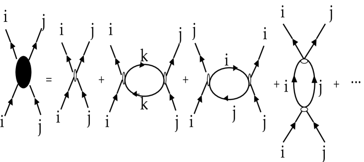
Figure 4: Some diagrams from a large-N theory

Figure 4 shows the first few diagrams in the expression for the scattering amplitude of particle of isospin index $i$ and $j$ in the Gross-Neveu theory. The “bare” vertex comes with a factor $\lambda/N$. The one-loop diagrams all share a factor $\lambda^{2}/N^{2}$ from the two vertices. The first one-loop diagram has a free internal summation over the index $k$ that runs over $N$ values, with the contribution being identical for each value of $k$. Thus, this one-loop diagram acquires a compensating factor of $N$ which makes its contribution of order $\lambda^{2}/N$, the same order in $1/N$ as the bare vertex. However, the other one-loop diagrams have no such free internal summation and their contribution is indeed of order $1/N^{2}$. Therefore, to leading order in $1/N$, one should keep only diagrams which have a free internal summation for every vertex, that is, iterates of the leading one-loop diagram, which are called bubble graphs. For later use remember that in the diagrams that survive (do not survive), the indices $i$ and $j$ of the incoming particles do not (do) enter the loops. Let us assume that the momentum integral up to the cutoff $\Lambda$ for one bubble gives a factor $-\Pi(\Lambda,q_{ext})$, where $q_{ext}$ is the external momentum or frequency transfer at which the scattering amplitude is evaluated. To leading order in large-$N$ the full expression for the scattering amplitude is

$$\Gamma(q_{ext})={1\over N}{\lambda\over 1+\lambda\Pi(\Lambda,q_{ext})}$$ (22)

Once one has the full expression for the scattering amplitude (to leading order in $1/N$) one can ask for the RG flow of the “bare” vertex as the cutoff is reduced by demanding that the physical scattering amplitude $\Gamma$ remain insensitive to the cutoff. One then finds (with $t=\ln(\Lambda_{0}/\Lambda)$)

$${d\Gamma(q_{ext})\over dt}=0\Rightarrow{d\lambda\over dt}=-\lambda^{2}{d\Pi(\Lambda,q_{ext})\over dt}$$ (23)

which is exactly the flow one would extract at one loop. Thus the one-loop RG flow is the exact answer to leading order in a large-$N$ theory. All higher-order corrections must therefore be subleading in $1/N$.

3.1 Large-N applied to Fermi liquids

Consider now the ${\bar{\psi}}\psi-{\bar{\psi}}\psi$ correlation function (with vanishing values of external frequency and momentum transfer). Landau showed that it takes the form

$$\chi={\chi_{0}\over 1+F_{0}},$$ (24)

where $F_{0}$ is the angular average of $F(\theta)$ and $\chi_{0}$ is the answer when $F=0$. Note that the answer is not perturbative in $F$.

Landau got this result by working with the ground-state energy as a functional of Fermi surface deformations. The RG provides us with not just the ground-state energy, but an effective hamiltonian (operator) for all of low-energy physics. This operator problem can be solved using large $N$-techniques.

The value of $N$ here is of order $K_{F}/\Lambda$, and here is how it enters the formalism. Imagine dividing the annulus in Fig. (1) into $N$ patches of size $(\Lambda)$ in the radial and angular directions. The momentum of each fermion ${\bf k}_{i}$ is a sum of a ”large” part ($\mathcal{O}(k_{F}))$ centered on a patch labelled by a patch index $i=1,...N$ and a ”small” momentum $(\mathcal{O}(\Lambda)$ within the patchrmprg .

Consider a four-fermion Green’s function, as in Figure (4). The incoming momenta are labelled by the patch index (such as $i$) and the small momentum is not shown but implicit. We have seen that as $\Lambda\to 0$, the two outgoing momenta are equal to the two incoming momenta up to a permutation. At small but finite $\Lambda$ this means the patch labels are same before and after. Thus the patch index plays the role of a conserved isospin index as in the Gross-Neveu model.

The electron-electron interaction terms, written in this notation, (with ${\mathbf{k}}$ integrals replaced by a sum over patch index and integration over small momenta) also come with a pre-factor of $1/N$ ($\simeq\Lambda/K_{F}$).

It can then be verified that in all Feynman diagrams of this cut-off theory the patch index plays the role of the conserved isospin index exactly as in a theory with $N$ fermionic species. For example in Figure (4) in the first diagram, the external indices $i$ and $j$ do not enter the diagram (small momentum transfer only) and so the loop momentum is nearly same in both lines and integrated fully over the annulus, i.e., the patch index $k$ runs over all $N$ values. In the second diagram, the external label $i$ enters the loop and there is a large momentum transfer ($\mathcal{O}({K_{F}}))$. In order for both momenta in the loop to be within the annulus, and to differ by this large $q$, the angle of the loop momentum is limited to a range $\mathcal{O}(\Lambda/K_{F})$. (This just means that if one momentum is from patch $i$ the other has to be from patch $j$. ) Similarly, in the last loop diagram, the angle of the loop momenta is restricted to one patch. In other words, the requirement that all loop momenta in this cut-off theory lie in the annulus singles out only diagrams that survive in the large $N$ limit.

The sum of bubble diagrams, singled out by the usual large-$N$ considerations, reproduces Landau’s Fermi liquid theory. For example in the case of $\chi$, one obtains a geometric series that sums to give $\chi={\chi_{0}\over 1+F_{0}}.$

Since in the large $N$ limit, the one-loop $\beta$-function for the fermion-fermion coupling is exact, it follows that the marginal nature of the Landau parameters $F$ and the flow of $V$ , Eqn. (20), are both exact as $\Lambda\to 0$.

A long paper of mine Ref. (rmprg ) explains all this, as well as how it is to be generalized to anisotropic Fermi surfaces and Fermi surfaces with additional special features and consequently additional instabilities. Polchinski pol independently analyzed the isotropic Fermi liquid (though not in the same detail, since it was a just paradigm or toy model for an effective field theory for him).

4 Quantum dots

We will now apply some of these ideas, very successful in the bulk, to two-dimensional quantum dotsqd-reviews ; aleiner - tiny spatial regions of size $L\simeq 100-200nm$, to which electrons are restricted using gates. The dot can be connected weakly or strongly to leads. Since many experts on dots are contributing to this volume, I will be sparing in details and references.

Let us get acquainted with some energy scales, starting with $\Delta$, the mean single particle level spacing. The Thouless energy is defined as $E_{T}={\hbar/\tau}$, where $\tau$ is the time it takes to traverse the dot. If the dot is strongly coupled to leads, this is the uncertainty in the energy of an electron as it traverses the dot. Consequently the $g$ (sharply defined) states of an isolated dot within $E_{T}$ will contribute to conductance and lead to a (dimensionless) conductance $g={E_{T}\over\Delta}$.

The dots in question have two features important to us. First, motion within the dot is ballistic: $L_{el}$, the elastic scattering length is the same as $L$, the dot size, so that $E_{T}={\hbar v_{F}\over L}$, where $v_{F}$ is the Fermi velocity. Next, the boundary of the dot is sufficiently irregular as to cause chaotic motion at the classical level. At the quantum level single-particle energy levels and wavefunctions (in any basis) within $E_{T}$ of the Fermi energy will resemble those of a random hamiltonian matrix and be described Random Matrix Theory (RMT) RMT . We will only invoke a few results from RMT and they will be explained in due course.

At a generic value of gate voltage $V_{g}$ the ground state has a definite number of particles $N$ and energy $\mathcal{E}_{N}$. If ${\mathcal{E}}_{N+1}-{\mathcal{E}}_{N}=\alpha eV_{g}$ ($\alpha$ is a geometry-dependent factor) the energies of the $N$ and $N+1$-particle states are degenerate, and a tunnelling peak occurs at zero bias. Successive peaks are separated by the second difference of ${\mathcal{E}}_{N}$, called $\Delta_{2}$, the distribution of which is measured. Also measured are statistics of peak-height distributionspeak-height-th ,peak-height-expt ; peak-height-expt2 , which depend on wavefunction statistics of RMT.

To describe the data one needs to write down a suitable hamiltonian

$$H_{U}=\sum\limits_{{\alpha}}{\varepsilon}_{\alpha}c^{\dagger}_{{\alpha}}c_{{\alpha}}+{1\over 2}\sum_{{\alpha}{\beta}{\gamma}{\delta}}V_{{\alpha}{\beta}{\gamma}{\delta}}c^{{\dagger}}_{{\alpha}}c^{{\dagger}}_{{\beta}}c_{{\gamma}}c_{{\delta}}$$ (25)

(where the subscripts label the exact single particle states including spin) and try to extract its implications. Earlier theoretical investigations were confined to the noninteracting limit: $V\equiv 0$ and missed the fact that due to the small capacitance of the dot, adding an electron required some significant charging energy on top of the energy of order ${\varepsilon}_{\alpha}$ it takes to promote an electron by one level. Thus efforts have been made to include interactionscoulomb-blockade ; H_U-prehistory ; H_U-kurland ; aleiner ; qd-numerics .

The simplest model includes a constant charging energy $U_{0}N^{2}/2$ coulomb-blockade ; qd-reviews . Conventionally $U_{0}$ is subtracted away in plotting $\Delta_{2}$. This model predicts a bimodal distribution for $\Delta_{2}$: Adding an electron above a doubly-filled (spin-degenerate) level costs $U_{0}+{\varepsilon}$, with ${\varepsilon}$ being the energy to the next single-particle level. Adding it to a singly occupied level costs $U_{0}$. While the second contribution gives a delta-function peak at $0$ after $U_{0}$ has been subtracted, the first contribution is the distribution of nearest neighbor level separation ${\varepsilon}$, of the order of $\Delta$. But simulations qd-numerics and experimentssmall-rs-expt ; large-rs-expt produce distributions for $\Delta_{2}$ which do not show any bimodality, and are much broader.

The next significant advance was the discovery of the Universal Hamiltonian H_U-prehistory ; H_U-kurland . Here one keeps only couplings of the form $V_{{\alpha}{\beta}{\beta}{\alpha}}$ on the grounds that only they have a non-zero ensemble average (over disorder realizations). This seems reasonable in the limit of large $g$ since couplings with zero average are typically of size $1/g$ according to RMT. The Universal Hamiltonian is thus

$$H_{U}=\sum\limits_{{\alpha},s}{\varepsilon}_{\alpha}c^{\dagger}_{{\alpha},s}c_{{\alpha},s}+{U_{0}\over 2}{N}^{2}-{J\over 2}{{\mathbf{S}}}^{2}+\lambda\bigg{(}\sum\limits_{{\alpha}}c^{\dagger}_{{\alpha},\uparrow}c^{\dagger}_{{\alpha},\downarrow}\bigg{)}\bigg{(}\sum\limits_{{\beta}}c_{{\beta},\downarrow}c_{{\beta},\uparrow}\bigg{)}$$ (26)

where $s$ is single-particle spin and ${{\mathbf{S}}}$ is the total spin. The Cooper coupling $\lambda$ does not play a major role, but the inclusion of the exchange coupling $J$ brings the theoretical predictionsH_U-prehistory ; H_U-kurland ; aleiner into better accord with experiments, especially if one-body “scrambling”scrambling ; adametal ; 2brim ; tau2 and finite temperature effects are taken into account. However, some discrepancies still remain in relation to numericalqd-numerics and experimental resultslarge-rs-expt at $r_{s}\geq 2$.

We now see that the following dot-related questions naturally arise. Given that adding more refined interactions (culminating in the universal hamiltonian) led to better descriptions of the dot, should one not seek a more systematic way to to decide what interactions should be included from the outset? Does our past experience with clean systems and bulk systems tell us how to proceed? Once we have written down a comprehensive hamiltonian, is there a way to go beyond perturbation theory to unearth nonperturbative physics in the dot, including possible phases and transitions between them? What will be the experimental signatures of these novel phases and the transitions between them if indeed they do exist? These questions will now be addressed.

4.1 Interactions and Disorder: Exact results on the dot

The first crucial step towards this goal was taken by Murthy and Mathur qd-us1 . Their ideas was as follows.

• Step 1: Use the clean system RG described earlier rmprg (eliminating momentum states on either side of the Fermi surface ) to eliminate all states far from the Fermi surface till one comes down to the Thouless band, that is, within $E_{T}$ of $E_{F}$.

  We have seen that this process inevitably leads to Landau’s Fermi liquid interaction (spin has been suppressed):

  $$V=\sum\limits_{m=0}^{\infty}{u_{m}\Delta\over 2}\sum\limits_{k,k^{\prime}}\cos[m({\theta}-{\theta}^{\prime})]c^{\dagger}_{{\mathbf{k}}}c_{{\mathbf{k}}}c^{\dagger}_{{\mathbf{k}}^{\prime}}c_{{\mathbf{k}}^{\prime}}$$ (27)

  where ${\theta},{\theta}^{\prime}$ are the angles of ${\mathbf{k}},\ {\mathbf{k}}^{\prime}$ on the Fermi circle, and $u_{m}$ is defined by

  $$F(\theta)=\sum_{m}u_{m}e^{im\theta}.$$ (28)

  A few words before we proceed. First, some experts will point out that the interaction one gets from the RG allows for small momentum transfer, i.e., there should be an additional sum over a small values $q$ in Eqn. (27) allowing ${\mathbf{k}}\to{\mathbf{k}}+{\mathbf{q}}$ and ${\mathbf{k}}^{\prime}\to{\mathbf{k}}^{\prime}-{\mathbf{q}}$. It can be shown that in the large $g$ limit this sum has just one term, at $q=0$. Unlike in a clean system, there is no singular behavior associated with $q\to 0$ and this assumption is a good one. Others have asked how one can introduce the Landau interaction that respects momentum conservation in a dot that does not conserve momentum or anything else except energy. To them I say this. Just think of a pair of molecules colliding in a room. As long as the collisions take place in a time scale smaller than the time between collisions with the walls, the interaction will be momentum conserving. That this is true for a collision in the dot for particles moving at $v_{F}$, subject an interaction of range equal to the Thomas Fermi screening length (the typical range) is readily demonstrated. Like it or not, momentum is a special variable even in a chaotic but ballistic dot since it is tied to translation invariance, and that that is operative for realistic collisions within the dot.

• Step 2: Switch to the exact basis states of the chaotic dot, writing the kinetic and interaction terms in this basis. Run the RG by eliminating exact energy eigenstates within $E_{T}$.

While this looks like a reasonable plan, it is not clear how it is going to be executed since knowledge of the exact eigenfunctions is needed to even write down the Landau interaction in the disordered basis:

$$V_{\alpha\beta\gamma\delta}= {\Delta\over 4}\sum\limits_{{\mathbf{k}}{\mathbf{k}}^{\prime}}u(\theta-\theta^{\prime})\left[\phi^{*}_{\alpha}({\mathbf{k}})\phi^{*}_{\beta}({\mathbf{k}}^{\prime})-\phi^{*}_{\alpha}({\mathbf{k}}^{\prime})\phi^{*}_{\beta}({\mathbf{k}})\right]$$ (29)

$$\times\left[\phi_{\gamma}({\mathbf{k}}^{\prime})\phi_{\delta}({\mathbf{k}})-\phi_{\gamma}({\mathbf{k}})\phi_{\delta}({\mathbf{k}}^{\prime})\right]$$

where ${\mathbf{k}}$ and ${\mathbf{k}}^{\prime}$ take $g$ possible values. These are chosen as follows. Consider the momentum states of energy within $E_{T}$ of $E_{F}$. In a dot momentum is defined with an uncertainty $\Delta k\simeq 1/L$ in either direction. Thus one must form packets in $k$ space obeying this condition. It can be easily shown that $g$ of them will fit into this band. One way to pick such packets is to simply take plane waves of precise ${\mathbf{k}}$ and chop them off at the edges of the dot and normalize the remains. The $g$ values of ${\mathbf{k}}$ can be chosen with an angular spacing $2\pi/g$. It can be readily verified that such states are very nearly orthogonal. The wavefunction $\phi_{\delta}({\mathbf{k}})$ is the projection of exact dot eigenstate $\delta$ on the state ${\mathbf{k}}$ as defined above.

We will see that one can go a long way without detailed knowledge of the wavefunctions $\phi_{\delta}({\mathbf{k}})$.

First, one can take the view of the Universal Hamiltonian (UH) adherents and consider the ensemble average (enclosed in $<>$ ) of the interactions. RMT tells us that to leading order in $1/g$,

$$<\phi_{\alpha}^{*}({\mathbf{k}}_{1})\phi_{\beta}^{*}({\mathbf{k}}_{2})\phi_{\gamma}({\mathbf{k}}_{3})\phi_{\delta}({\mathbf{k}}_{4})> ={{\delta}_{{\alpha}{\delta}}{\delta}_{{\beta}{\gamma}}{\delta}_{{\mathbf{k}}_{1}{\mathbf{k}}_{4}}{\delta}_{{\mathbf{k}}_{2}{\mathbf{k}}_{3}}\over g^{2}}+{{\delta}_{{\alpha}{\gamma}}{\delta}_{{\beta}{\delta}}{\delta}_{{\mathbf{k}}_{1}{\mathbf{k}}_{3}}{\delta}_{{\mathbf{k}}_{2}{\mathbf{k}}_{4}}\over g^{2}}$$ (30)

$$+{{\delta}_{{\alpha}{\beta}}{\delta}_{{\gamma}{\delta}}{\delta}_{{\mathbf{k}}_{1},-{\mathbf{k}}_{2}}{\delta}_{{\mathbf{k}}_{3},-{\mathbf{k}}_{4}}\over g^{2}}$$

It is seen that only matrix elements in Eqn. (29) for which the indices ${\alpha}{\beta}{\gamma}{\delta}$ are pairwise equal survive disorder-averaging, and also that the average has no dependence on the energy of ${\alpha}{\beta}{\gamma}{\delta}$. In the spinless case, the first two terms on the right hand side make equal contributions and produce the constant charging energy in the Universal Hamiltonian of Eq. (26), while in the spinful case they produce the charging and exchange terms. The final term of Eq. (30) produces the Cooper interaction of Eq. (26).

Thus the UH contains the rotationally invariant part of the Landau interaction. The others, i.e., those that do not survive ensemble averaging, are dropped because they are of order $1/g$. But we have seen before in the BCS instability of the Fermi liquid that a term that is nominally small to begin with can grow under the RG. That this is what happens in this case was shown by the RG calculation of Murthy and Mathur. There was however one catch. The neglected couplings could overturn the UH description for couplings that exceeded a critical value. However the critical value is of order unity and so one could not trust either the location or even the very existence of this critical point based on their perturbative one-loop calculation. Their work also gave no clue as to what lay on the other side of the critical point.

Subsequently Murthy and I qd-us2 showed that the methods of the large $N$ theories (with $g$ playing the role of $N$) were applicable here and could be used to show nonperturbatively in the interaction strength that the phase transition indeed exists. This approach also allowed us to study in detail the phase on the other side of the transition, as well as what is called the quantum critical region, to be described later.

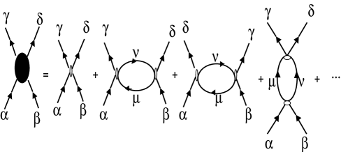
Figure 5: Feynman diagrams for the full four-point amplitude $\Gamma_{{\alpha}{\beta}{\gamma}{\delta}}$.

Let us now return to Murthy and Mathur and ask how the RG flow is derived. After integrating some of the $g$ states within $E_{T}$, we end up with $g^{\prime}=ge^{-t}$ states. Suppose we compute a scattering amplitude $\Gamma_{{\alpha}{\beta}{\gamma}{\delta}}$ for the process in which two fermions originally in states ${\alpha}{\beta}$ are scattered into states ${\gamma}{\delta}$. This scattering can proceed directly through the vertex $V_{{\alpha}{\beta}{\gamma}{\delta}}(t)$, or via intermediate virtual states higher order in the interactions, which can be classified by a set of Feynman diagrams, as shown in Figure 5. All the states in the diagrams belong to the $g^{\prime}$ states kept. We demand that the entire amplitude be independent of $g^{\prime}$, meaning that the physical amplitudes should be the same in the effective theory as in the original theory. This will lead to a set of flow equations for the $V_{{\alpha}{\beta}{\gamma}{\delta}}$. In principle this flow equation will involve all powers of $V$ but we will keep only quadratic terms (the one-loop approximation). Then the diagrams are limited to the ones shown in Figure 5, leading to the following contributions to the scattering amplitude $\Gamma_{{\alpha}{\beta}{\gamma}{\delta}}$

$$\Gamma_{{\alpha}{\beta}{\gamma}{\delta}}= V_{{\alpha}{\beta}{\gamma}{\delta}}$$

$$+ \sum\limits_{\mu,\nu}{}^{\prime}{N_{F}(\nu)-N_{F}(\mu)\over{\varepsilon}_{\mu}-{\varepsilon}_{\nu}}(V_{{\alpha}\nu\mu{\delta}}V_{{\beta}\mu\nu{\gamma}}-V_{{\alpha}\nu\mu{\gamma}}V_{{\beta}\mu\nu{\delta}})$$

$$- \sum\limits_{\mu\nu}{}^{\prime}{1-N_{F}(\mu)-N_{F}(\nu)\over{\varepsilon}_{\mu}+{\varepsilon}_{\nu}}V_{{\alpha}{\beta}\mu\nu}V_{\nu\mu{\gamma}{\delta}}$$ (31)

where the prime on the sum reminds us that only the $g^{\prime}$ remaining states are to be kept and where $N_{F}({\alpha})$ is the Fermi occupation of the state ${\alpha}$. We will confine ourselves to zero temperature where this number can only be zero or one. The matrix element $V_{{\alpha}{\beta}{\gamma}{\delta}}$ now explicitly depends on the RG flow parameter $t$.

Now we demand that upon integrating the two states at $\pm g^{\prime}\Delta/2$ we recover the same $\Gamma_{{\alpha}{\beta}{\gamma}{\delta}}$. Clearly, since $g^{\prime}=ge^{-t}$,

$${d\over dt}=-g^{\prime}{{\delta}\over{\delta}g^{\prime}}$$ (32)

The effect of this differentiation on the loop diagrams is to fix one of the internal lines of the loop to be at the cutoff $\pm g^{\prime}\Delta/2$, while the other one ranges over all smaller values of energy. In the particle-hole diagram, since $\mu$ or $\nu$ can be at $+g^{\prime}\Delta/2$ or $-g^{\prime}\Delta/2$, and the resulting summations are the same in all four cases, we take a single contribution and multiply by a factor of 4. The same reasoning applies to the Cooper diagram. Let us define the energy cutoff $\Lambda=g^{\prime}\Delta/2$ to make the notation simpler. Since we are integrating out two states we have ${\delta}g^{\prime}=2$

$$0= {dV_{{\alpha}{\beta}{\gamma}{\delta}}\over dt}$$

$$- {g^{\prime}\over 2}4\sum\limits_{\mu=\Lambda,\nu}{}^{\prime}{N_{F}(\nu)-N_{F}(\mu)\over{\varepsilon}_{\mu}-{\varepsilon}_{\nu}}(V_{{\alpha}\nu\mu{\delta}}V_{{\beta}\mu\nu{\gamma}}-V_{{\alpha}\nu\mu{\gamma}}V_{{\beta}\mu\nu{\delta}})$$

$$+ {g^{\prime}\over 2}4\sum\limits_{\mu=\Lambda,\nu}{}^{\prime}{1-N_{F}(\mu)-N_{F}(\nu)\over{\varepsilon}_{\mu}+{\varepsilon}_{\nu}}V_{{\alpha}{\beta}\mu\nu}V_{\nu\mu{\gamma}{\delta}}$$ (33)

where $\mu=\Lambda$ means $\varepsilon_{\mu}=\Lambda$ and so on. The changed sign in front of the 1-loop diagrams reflects the sign of Eq. (32)

So far we have not made any assumptions about the form of $V_{{\alpha}{\beta}{\gamma}{\delta}}$, and the formulation applies to any finite system. In a generic system such as an atom, the matrix elements depend very strongly on the state being integrated over, and the flow must be followed numerically for each different set ${\alpha}{\beta}{\gamma}{\delta}$ kept in the low-energy subspace.

In our problem things have become so bad that are good once again: the wavefunctions $\phi({\mathbf{k}})$ that enter the matrix elements above have so scrambled up by disorder that they can be handled by RMT. In particular it is possible to argue that the sum over the $g^{\prime}$ terms may be replaced by it ensemble average. In other words the flow equation is self-averaging. While the most convincing way to show this is to compute its variance, and see that it is of order $1/\sqrt{g}$ times its average, this fact can be motivated in the following way: There is a sum over $g^{\prime}\gg 1$ values of $\nu$ with a slowly varying energy denominator, which makes the sum over $\nu$ similar to a spectral average, which in RMT is the same as an average over the disorder ensemble. A more sophisticated argument is presented in Ref gang4 . We can use the result

$$<\phi^{*}_{\mu}({\mathbf{p}}_{1})\phi^{*}_{\nu}({\mathbf{p}}_{2})\phi_{\nu}({\mathbf{p}}_{3})\phi_{\mu}({\mathbf{p}}_{4})>=$$

$${{\delta}_{14}{\delta}_{23}\over g^{2}}-{{\delta}_{13}{\delta}_{24}\over g^{3}}-{{\delta}_{1,-2}{\delta}_{3,-4}\over g^{3}}$$ (34)

to deal with the product of four wavefunctions inside the loop and deal with the energy sum as follows:

$$\sum\limits_{{\varepsilon}_{\nu}=-\Lambda}^{0}{1\over\Lambda+|{\varepsilon}_{\nu}|}\approx\int\limits_{0}^{\Lambda}{d{\varepsilon}\over\Delta}{1\over\Lambda+{\varepsilon}}={\ln{2}\over\Delta}$$ (35)

We are exploiting the fact that wavefunction correlations are energy independent in the large -$g$ limit.

After we make this simplifications we find that there are many kinds of terms of which one kind dominates in the large -$g$ limit.

Let us go back to the properly antisymmetrized matrix element defined in terms of the Fermi liquid interaction function, Eq. (29). Since there is a product of two $V$’s in each loop diagram, and each $V$ contains 4 terms, it is clear that each loop contribution has 16 terms. Let us first consider a term of the leading type in the particle-hole diagram, which survives in the large-$g$ limit. Putting in the full wavefunction dependencies (and ignoring factors other than $g,\ g^{\prime}$) we have the following contribution from this type of term

$${dV_{{\alpha}{\beta}{\gamma}{\delta}}\over dt}_{\mbox{Leading}}= g^{\prime}\Delta^{2}\sum\limits_{\nu=-\Lambda}^{0}{1\over\Lambda+|{\varepsilon}_{\nu}|}\sum\limits_{{\mathbf{k}}{\mathbf{k}}^{\prime}}\sum\limits_{{\mathbf{p}}{\mathbf{p}}^{\prime}}u({\theta}_{\mathbf{k}}-{\theta}_{\mathbf{p}})u({\theta}_{{\mathbf{p}}^{\prime}}-{\theta}_{{\mathbf{k}}^{\prime}})$$ (36)

$$\times\phi^{*}_{\alpha}({\mathbf{k}})\phi^{*}_{\beta}({\mathbf{k}}^{\prime})\phi_{\gamma}({\mathbf{k}}^{\prime})\phi_{\delta}({\mathbf{k}})\phi^{*}_{\mu}({\mathbf{p}})\phi^{*}_{\nu}({\mathbf{p}}^{\prime})\phi_{\nu}({\mathbf{p}})\phi_{\mu}({\mathbf{p}}^{\prime})$$

Substituting the appropriate momentum labels for the particle-hole diagram in Eqn. (34), we see that the wavefunction average relevant to the sum over intermediate states is

$${{\delta}_{{\mathbf{p}}{\mathbf{p}}^{\prime}}\over g^{2}}-{1+{\delta}_{{\mathbf{p}},-{\mathbf{p}}^{\prime}}\over g^{3}}$$ (37)

Using the self-averaging, the first term of Eq.(37) forces ${\mathbf{p}}={\mathbf{p}}^{\prime}$ in Eq. (36). For large $g$, using

$$\sum\limits_{{\mathbf{p}}}=g\int{d{\theta}_{\mathbf{p}}\over 2\pi}$$ (38)

we obtain a convolution of the two Fermi liquid functions

$$\sum\limits_{{\mathbf{p}}}u({\theta}_{\mathbf{k}}-{\theta}_{\mathbf{p}})u({\theta}_{\mathbf{p}}-{\theta}_{{\mathbf{k}}^{\prime}})=g\big{(}u_{0}^{2}+{1\over 2}\sum\limits_{m=1}^{\infty}u_{m}^{2}\cos{m({\theta}-{\theta}^{\prime})}\big{)}$$ (39)

where we have reverted to the notation ${\theta}={\theta}_{\mathbf{k}},\ {\theta}^{\prime}={\theta}_{{\mathbf{k}}^{\prime}}$. In the second term of Eq. (37), the ${\delta}_{{\mathbf{p}},-{\mathbf{p}}^{\prime}}$ turns out to be subleading, while the other allows independent sums over ${\mathbf{p}},\ {\mathbf{p}}^{\prime}$. This means that only $u_{0}$ contributes to this term, (other avrerage to zero upon summing over all angles) which produces

$$-\sum\limits_{{\mathbf{p}}{\mathbf{p}}^{\prime}}u({\theta}_{\mathbf{k}}-{\theta}_{\mathbf{p}})u({\theta}_{{\mathbf{p}}^{\prime}}-{\theta}_{{\mathbf{k}}^{\prime}})=g^{2}u_{0}^{2}$$ (40)

Feeding this into full expression for this contribution to the particle-hole diagram, we find it to be

$${dV_{{\alpha}{\beta}{\gamma}{\delta}}\over dt}_{\mbox{Leading}}= {g^{\prime}\over g}\Delta\ln{2}\sum\limits_{{\mathbf{k}}{\mathbf{k}}^{\prime}}\bigg{(}\sum\limits_{m=1}^{\infty}u_{m}^{2}\cos{m({\theta}-{\theta}^{\prime})}\bigg{)}$$ (41)

$$\phi^{*}_{\alpha}({\mathbf{k}})\phi^{*}_{\beta}({\mathbf{k}}^{\prime})\phi_{\gamma}({\mathbf{k}}^{\prime})\phi_{\delta}({\mathbf{k}})$$

Notice that the result is still of the Fermi liquid form. In other words the couplings $V_{{\alpha}{\beta}{\gamma}{\delta}}$ which were written in terms of Landau parameters $u_{m}$, flow into renormalized coupling once again expressible in terms of renormalized Landau parameters. By comparing the two sides, we see each $u_{m}$ flows independently of the others as per

$${du_{m}\over dt}=-e^{-t}(\ln{2})u_{m}^{2}\ \ \ \ \ \ \ \ m\neq 0$$ (42)

The above equation can be written in a more physically transparent form by using a rescaled variable (for $m\neq 0$ only)

$${\tilde{u}}_{m}=e^{-t}u_{m}$$ (43)

in terms of which the flow equation becomes

$${d{\tilde{u}}_{m}\over dt}=-{\tilde{u}}_{m}-(\ln{2}){\tilde{u}}_{m}^{2}\equiv\beta({\tilde{u}}_{m})$$ (44)

where the last is a definition of the ${\beta}$-function.

The reason $u_{o}$ does not flow is that the corresponding interaction commutes with the one-body “kinetic” part, and therefore does not suffer quantum fluctuations.

This is the answer at large $g$. We have dropped subleading contributions of the following type:

$${dV_{{\alpha}{\beta}{\gamma}{\delta}}\over dt}|_{\mbox{sub}} =-g^{\prime}\Delta^{2}\sum\limits_{\nu=-\Lambda}^{0}{1\over\Lambda+|{\varepsilon}_{\nu}|}\left[\sum\limits_{{\mathbf{k}}{\mathbf{k}}^{\prime}}\sum\limits_{{\mathbf{p}}{\mathbf{p}}^{\prime}}u({\theta}_{\mathbf{k}}-{\theta}_{\mathbf{p}})u({\theta}_{{\mathbf{p}}^{\prime}}-{\theta}_{{\mathbf{k}}^{\prime}})\ \right.$$ (45)

$$\left.\times\phi^{*}_{\alpha}({\mathbf{p}})\phi^{*}_{\beta}({\mathbf{k}}^{\prime})\phi_{\gamma}({\mathbf{k}}^{\prime})\phi_{\delta}({\mathbf{k}})\phi^{*}_{\mu}({\mathbf{k}})\phi^{*}_{\nu}({\mathbf{p}}^{\prime})\phi_{\nu}({\mathbf{p}})\phi_{\mu}({\mathbf{p}}^{\prime})\right]$$

Note that the momentum labels of $\phi^{*}_{\alpha}$ and $\phi^{*}_{\mu}$ have been exchanged compared to Eq. (36) and there is a minus sign, both coming from the antisymmetrization of Eq. (29). Once again we ensemble average the internal $\mu,\ \nu$ sum, the wavefunction part of which gives

$$<\phi^{*}_{\mu}({\mathbf{k}})\phi^{*}_{\nu}({\mathbf{p}}^{\prime})\phi_{\nu}({\mathbf{p}})\phi_{\mu}({\mathbf{p}}^{\prime})>={{\delta}_{{\mathbf{k}}{\mathbf{p}}^{\prime}}{\delta}_{{\mathbf{p}}{\mathbf{p}}^{\prime}}\over g^{2}}-{{\delta}_{{\mathbf{k}}{\mathbf{p}}}+{\delta}_{{\mathbf{k}},-{\mathbf{p}}^{\prime}}{\delta}_{{\mathbf{p}},-{\mathbf{p}}^{\prime}}\over g^{3}}$$ (46)

It is clear that there is an extra momentum restriction in each term compared to Eq. (37), which means that one can no longer sum freely over ${\mathbf{p}}$ to get the factor of $g$ in Eq. (39), or the factor of $g^{2}$ in Eq. (40). Therefore this contribution will be down by $1/g$ compared to that of Eq. (36).

Turning now to the Cooper diagrams, the internal lines are once again forced to have the same momentum labels as the external lines by the Fermi liquid vertex, therefore they do not make any leading contributions.

The general rule is that whenever a momentum label corresponding to an internal line in the diagram (here $\mu$ and $\nu$) is forced to become equal to a momentum label corresponding to an external disorder label (here ${\alpha},{\beta},{\gamma},$ or ${\delta}$), the diagram is down by $1/g$, exactly as in the $1/N$ expansion. The fact that $1/g$ plays the role of $1/N$ was first realized by Murthy and Shankar qd-us2 . Not only did this mean that the one loop flow of Murthy and Mathur was exact, it meant the disorder-interaction problem of the chaotic dot could be solved exactly in the large $g$ limit. It is the only known case where the problem of disorder and interactionsintdisorder ; belitz ; weak-ferro can be handled exactly.

From Eqn. (44) it can be seen that positive initial values of ${\tilde{u}}_{m}$ (which are equal to initial values of $u_{m}$ inherited from the bulk) are driven to the fixed point at ${\tilde{u}}_{m}=0$, as are negative initial values as long as $u_{m}(t=0)\geq u_{m}^{*}=-1/\ln{2}$. Thus, the Fermi liquid parameters are irrelevant for this range of starting values. Recall that setting all $u_{m}=0$ for $m\neq 0$ results in the Universal Hamiltonian. Thus, the range $u_{m}\geq u_{m}^{*}$ is the basin of attraction of the Universal Hamiltonian. On the other hand, for $u_{m}(t=0)\leq u_{m}^{*}$ results in a runaway flow towards large negative values of $u_{m}$, signalling a transition to a phase not perturbatively connected to the Universal Hamiltonian.

Since we have a large $N$ theory here (with $N=g$), the one-loop flow and the new fixed point at strong coupling are parts of the final theory. What is the nature of the state for $u_{m}(t=0)\leq u_{m}^{*}$? The formalism and techniques needed to describe that are beyond what was developed in these lectures, which has focused on the RG. Suffice it to say that it is possible to write the partition function in terms of a new collective field $\sigma$ (which depends on all the particles) and that the action $S(\mbox{\boldmath$\sigma$})$ has a factor $g$ in front of it, allowing us to evaluate the integral by saddle point(in the limit $g\to\infty$), to confidently predict the strong coupling phase and many of its properties. Our expectations based on the large $g$ analysis have been amply confirmed by detailed numerical studies gang4 . For now I will briefly describe the new phenomenon in qualitative terms for readers not accustomed to these ideas and give some references for those who are.

In the strong coupling region $\sigma$ acquires an expectation value in the ground state. The dynamics of the fermions is affected by this variable in many ways: quasi-particle widths become broad very quickly above the Fermi energy, the second difference $\Delta_{2}$ has occasionally very large values and can even be negative, , and the system behaves like one with broken time-reversal symmetry if $m$ is odd.

Long ago Pomeranchuk pomeranchuk found that if a Landau function of a pure system exceeded a certain value, the fermi surface underwent a shape transformation from a circle to an non-rotationally invariant form. Recently this transition has received a lot of attentionvarma ; oganeysan The transition in question is a disordered version of the same. Details are given in Refs. (qd-us2 , gang4 ).

Details aside, there is another very interesting point: even if the coupling does not take us over to the strong-coupling phase, we can see vestiges of the critical point $u_{m}^{*}$ and associated critical phenomena. This is a general feature of many quantum critical pointscritical-fan , i.e., points like $u_{m}^{*}$ where as a variable in a hamiltonian is varied, the system enters a new phase (in contrast to transitions wherein temperature $T$ is the control parameter).

Figure 6 shows what happens in a generic situation. On the $x$-axis a variable ($u_{m}$ in our case ) along which the quantum phase transition occurs. Along $y$ is measured a new variable, usually temperature $T$. Let us consider that case first. If we move from right to left at some value of $T$, we will first encounter physics of the weak-coupling phase determined by the weak-coupling fixed point at the origin. Then we cross into the critical fan (delineated by the $V$-shaped dotted lines), where the physics controlled by the quantum critical point. In other words we can tell there is a critical point on the $x$ -axis without actually traversing it. As we move further to the left, we reach the strongly-coupled symmetry-broken phase, with a non-zero order parameter.

It can be shown that in our problem, $1/g$ plays the role of $T$. One way to see is this that in any large $N$ theory $N$ stands in front of the action when written in terms of the collective variable. That is true in this case well for $g$. (Here $g$ also enters at a subdominant level inside the action, which makes it hard to predict the exact shape of the critical fan. The bottom line is that we can see the critical point at finite $1/g$. In addition one can also raise temperature or bias voltage to see the critical fan.

Subsequent work has shown, in more familiar examples that Landau interactions, that the general picture depicted here is true in the large $g$ limit: upon adding sufficiently strong interactions the Universal Hamiltonian gives way to other descriptions with broken symmetrybrower ; gm .

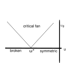
Figure 6: The generic phase diagram for a second-order quantum phase transition. The horizontal axis represents the coupling constant which can be tuned to take one across the transition. The vertical axis is usually the temperature in bulk quantum systems, but is $1/g$ here, since in our system one of the roles played by $g$ is that of the inverse temperature.

5 Acknowledgement

It is a pleasure to thank the organizers of this school especially Professors Dieter Heiss, Nithaya Chetty and Hendrik Geyer for their stupendous hospitality that made all of decide to revisit South Africa as soon as possible.

References

- (1) M.E.Fisher Critical Phenomena, F. W. J. Hahne, Editor, Lecture Notes Number 186, Springer-Verlag, Berlin, (1983). These notes are from the Engelbrecht Summer School of 1983!
- (2) R. Shankar, Physica A177, 530 (1991); R.Shankar, Rev. Mod. Phys. 66, 129 (1994).
- (3) L. D. Landau, Sov. Phys. JETP 3, 920 (1956); Sov. Phys. JETP 5, 101 (1957).
- (4) A. A. Abrikosov, L. P. Gorkov, and I. E. Dzyaloshinski, Methods of Quantum Field Theory in Statistical Physics, Dover Publications, New York, 1963.
- (5) D. J. Gross and A. Neveu, Phys. Rev.D10, 3235 (1974).
- (6) P.Polchinski In: TASI Elementary Particle Physics, ed by J. Polchinski and J.Harvey (World Scientific, 1992.)
- (7) For recent reviews, see, T. Guhr, A. Müller-Groeling, and H. A. Weidenmüller, Phys. Rep. 299, 189 (1998); Y. Alhassid, Rev. Mod. Phys. 72, 895 (2000); A. D. Mirlin, Phys. Rep. 326, 259 (2000).
- (8) M. L. Mehta, Random Matrices, Academic Press, San Diego, 1991. K. B. Efetov, Adv. Phys. 32, 53 (1983); B. L. Al’tshuler ad B. I. Shklovskii, Sov. Phys. JETP 64, 127 (1986).
- (9) I. L. Aleiner, P. W. Brouwer, and L. I. Glazman, Phys. Rep. 358, 309 (2002), and references therein; Y. Oreg, P. W. Brouwer, X. Waintal, and B. I. Halperin, cond-mat/0109541, “Spin, spin-orbit, and electron-electron interactions in mesoscopic systems”.
- (10) R. A. Jalabert, A. D. Stone, and Y. Alhassid, Phys. Rev. Lett.68, 3468 (1992).
- (11) A. M. Chang, H. U. Baranger, L. N. Pfeiffer, K. W. West, and T. Y. Chang, Phys. Rev. Lett.76, 1695 (1996); J. A. Folk, S. R. Patel, S. F. Godjin, A. G. Huibers, S. M. Cronenwett, and C. M. Marcus, Phys. Rev. Lett.76, 1699 (1996).
- (12) S. R. Patel, D. R. Stewart, C. M. Marcus, M. Gokcedag, Y. Alhassid, A. D. Stone, C. I. Dururoz, and J. S. Harris, Phys. Rev. Lett.81, 5900 (1998).
- (13) D. V. Averin and K. K. Likharev, in Mesoscopic Phenomena in Solids, edited by B. L. Altshuler, P. A. Lee, and R. Webb (Elsevier, Amsterdam, 1991); C. W. J. Beenakker, Phys. Rev. B44, 1646 (1991).
- (14) A. V. Andreev and A. Kamenev, Phys. Rev. Lett.81, 3199 (1998), P. W. Brouwer, Y. Oreg, and B. I. Halperin, Phys. Rev. B60, R13977 (1999), H. U. Baranger, D. Ullmo, and L. I. Glazman, Phys. Rev. B61, R2425 (2000).
- (15) I. L. Kurland, I. L. Aleiner, and B. L. Al’tshuler, Phys. Rev. B 62, 14886 (2000).
- (16) O. Prus, A. Auerbach, Y. Aloni, U. Sivan, and R. Berkovits, Phys. Rev. B54, R14289 (1996), R. Berkovits, Phys. Rev. Lett. 81, 2128 (1998), A. Cohen, K. Richter, and R. Berkovits, Phys. Rev. B 60, 2536 (1999), P. N. Walker, G. Montambaux, and Y. Gefen, ibid, 2541 (1999), S. Levit and D. Orgad, Phys. Rev. B 60, 5549 (1999), D. Ullmo and H. U. Baranger, Phys. Rev. B 64, 245324 (2001), V. Belinicher, E. Ginossar, and S. Levit, cond-mat/0109005, Y. Alhassid and S. Malhotra, cond-mat/0202453, .
- (17) U. Sivan et al, Phys. Rev. Lett. 77, 1123 (1996); S. R. Patel et al, Phys. Rev. Lett. 80, 4522 (1998).
- (18) F. Simmel et al, Phys. Rev. B 59, 10441 (1999); D. Abusch-Magder et al, Physica E 6, 382 (2000).
- (19) Y. M. Blanter, A. D. Mirlin, and B. A. Muzykantskii, Phys. Rev. Lett.78, 2449 (1997), R. O. Vallejos, C. H. Lewenkopf, and E. R. Mucciolo, Phys. Rev. Lett.81, 677 (1998), .
- (20) S. Adam, P. W. Brouwer, J. P. Sethna, and X. Waintal, cond-mat/0203002.
- (21) J. B. French and S. S. M. Wong, Phys. Lett. 33B, 447 (1970), ‘ O. Bohigas and J. Flores, Phys. Lett. 34B, 261 (1971), Y. Alhassid, Ph. Jacquod, and A. Wobst, Phys. Rev. B 61, 13357 (2000), Physica E 9, 393 (2001), Y. Alhassid and A. Wobst, Phys. Rev. B 65, 041304 (2002), .
- (22) A. Tscherich and K. B. Efetov, Phys. Rev.E62, 2042 (2000), .
- (23) G. Murthy and H. Mathur, Phys. Rev. Lett. 89, 126804 (2002).
- (24) G. Murthy and R. Shankar, Phys. Rev. Lett.90, 066801 (2003).
- (25) G Murthy, R. Shankar, Damir Herman, and Harsh Mathur, cond-mat 0306529, Phys. Rev. B69, 075321, (2004).
- (26) A. M. Finkel’shtein, Sov. Phys. JETP 57, 97 (1983); C. Castellani, C. Di Castro, P. A. Lee, and M. Ma, Phys. Rev. B30, 527 (1984).
- (27) For a review of the theory, see, D. Belitz and T. R. Kirkpatrick, Rev. Mod. Phys. 66, 261 (1994).
- (28) D. Belitz and T. R. Kirkpatrick, Phys. Rev. B53, 14364 (1996); C. de C. Chamon and E. Mucciolo, Phys. Rev. Lett.85, 5607 (2000); C. Nayak and X. Yang, cond-mat/0302503.
- (29) I. I. Pomeranchuk, Sov. Phys. JETP 8, 361 (1958).
- (30) C. M. Varma, Phys. Rev. Lett. 83, 3538 (1999).
- (31) V. Oganesyan, S. A. Kivelson, and E. Fradkin, Phys. Rev. B 64, 195109 (2001).
- (32) S. Chakravarty, B. I. Halperin, and D. R. Nelson, Phys. Rev. Lett. 60, 1057 (1988); Phys. Rev. B 39, 2344 (1989); For a detailed treatment of the generality of the phenomenon, see, S. Sachdev, Quantum Phase Transitions, Cambridge University Press, Cambridge 1999.
- (33) Shaffique Adam, Piet W. Brouwer, and Prashant Sharma Phys. Rev. B 68, 241311 (2003).
- (34) G. Murthy, Random Matrix Crossovers and Quantum Critical Crossovers for Interacting Electrons in Quantum Dotscond-mat-0406029.