Rapid rotation of a Bose-Einstein condensate in a harmonic plus quartic trap

Abstract

A two-dimensional rapidly rotating Bose-Einstein condensate in an anharmonic trap with quadratic and quartic radial confinement is studied analytically with the Thomas-Fermi approximation and numerically with the full time-independent Gross-Pitaevskii equation. The quartic trap potential allows the rotation speed $\Omega$ to exceed the radial harmonic frequency $\omega_{\perp}$. In the regime $\Omega\gtrsim\omega_{\perp}$, the condensate contains a dense vortex array (approximated as solid-body rotation for the analytical studies). At a critical angular velocity $\Omega_{h}$, a central hole appears in the condensate. Numerical studies confirm the predicted value of $\Omega_{h}$, even for interaction parameters that are not in the Thomas-Fermi limit. The behavior is also investigated at larger angular velocities, where the system is expected to undergo a transition to a giant vortex (with pure irrotational flow).

I Introduction

The development of experimental techniques to create a single vortex in a dilute trapped Bose-Einstein condensate (BEC) Matt99 ; Madi00 rapidly led to larger arrays containing up to several hundred vortices Abo01 ; Rama01 ; Halj01 ; Enge02 . Typically, these condensates rotate rapidly, with angular velocities $\Omega$ that approach the radial trap oscillator frequency $\omega_{\perp}$. The resulting centrifugal effect significantly weakens the radial confinement, so that the condensate expands radially and shrinks axially Rama01 ; Halj01 ; Fett01 .

In a pure harmonic radial trap, the limit $\Omega\to\omega_{\perp}$ is singular, because the Thomas-Fermi (TF) radius diverges and the central density decreases toward zero. Consequently, the angular momentum also diverges, and it becomes increasingly difficult to spin up the condensate as it approaches this limit. In addition, the single-particle Hamiltonian reduces to that of a charged particle in a uniform magnetic field Ho01 , and the ground state can be constructed from the lowest-Landau-level wave functions. Recent experiments have explored the crossover region between these two regimes Schw04 ; Codd04 .

One procedure that eliminates this singularity is to add a stronger radial potential that confines the condensate even for $\Omega\geq\omega_{\perp}$. A quartic potential provides a particularly simple form Fett01 ; Lund02 that has recently been realized experimentally with a blue-detuned laser directed along the axial direction Bret04 ; Stoc04 .

For this combined potential, the system is expected to have no vortices at sufficiently slow rotation speeds $\Omega$. With increasing $\Omega$, there is a sequence of states with an increasing number of vortices that eventually form a relatively large vortex lattice. This behavior is not qualitatively different from that in a pure harmonic trap. The new feature of the quartic confining potential is that the condensate continues to expand radially for $\Omega>\omega_{\perp}$, with a central hole appearing at a critical angular velocity $\Omega_{h}$. For still larger values of $\Omega$, the condensate has an annular form with a mean radius that continues to expand with increasing $\Omega$. Ultimately, a giant vortex is expected to appear when the singly quantized vortices disappear from the Thomas-Fermi condensate, leaving an axisymmetric state with pure irrotational flow in the annulus. One reason for the interest in the additional quartic potential is that the central hole and giant vortex do not occur for a pure harmonic trap potential.

Previous theoretical work on this system has been mainly numerical Kasa02 ; Kavo03 or for weak interactions and small anharmonicities Jack04 , and here we report an analytical study of the TF regime, approximating the actual superfluid velocity of the dense vortex array by solid-body rotation $\bm{v}_{\rm sb}=\bm{\Omega}\times\bm{r}$. In addition, we perform a full numerical study of the two-dimensional Gross-Pitaevskii equation for different interaction strengths. Comparison of the numerical and analytical studies confirms the qualitative features of the TF analysis. Section II summarizes the basic TF procedure. This approach predicts the critical angular velocity $\Omega_{h}$ for the initial appearance of a central hole, surrounded by a dense vortex lattice (Sec. III). The corresponding numerical study is described in Sec. IV, confirming the TF result for $\Omega_{h}$. For larger values of $\Omega>\Omega_{h}$, the TF approximation predicts that the annular condensate expands radially with constant area. Thus the width of the annulus decreases, and eventually the vortices are expected to retreat into the central hole (Sec. V), leaving a pure irrotational state with macroscopic circulation (often called a “giant vortex”) Kasa02 ; Kavo03 ; Fisc03 . Since solid-body rotation always minimizes the energy in the rotating frame, this transition to a giant vortex depends essentially on the discrete character of the quantized superfluid vortices. Comparison with our numerical studies shows that the theoretical analyses are less successful in modeling this transition Kavo03 .

II Summary of procedure

The problem of interest is the equilibrium state of a rapidly rotating trapped Bose-Einstein condensate in a two-dimensional confining potential that has both quadratic (harmonic) and quartic components. In terms of the usual dimensional quantities, the trap potential has the form

$$V_{\rm tr}(r)=\frac{1}{2}M\omega_{\perp}^{2}\left(r^{2}+\lambda\frac{r^{4}}{d_{\perp}^{2}}\right)=\frac{1}{2}\,\hbar\omega_{\perp}\left(\frac{r^{2}}{d_{\perp}^{2}}+\lambda\frac{r^{4}}{d_{\perp}^{4}}\right),$$ (1)

where $d_{\perp}=\sqrt{\hbar/M\omega_{\perp}}$ is the harmonic-oscillator length, $\bm{r}$ is the two-dimensional radial coordinate and $\lambda$ is a dimensionless constant that characterizes the admixture of the quartic component. For simplicity, it is convenient to treat an effectively two-dimensional system, uniform in the $z$ direction over a length $Z$. Kavoulakis and Baym Kavo03 considered the same two-dimensional system, especially in the limit of rapid rotation where the condensate develops a central hole and becomes annular.

In a frame rotating with angular velocity $\Omega$, the energy is given by the functional

$$E^{\prime}=\int dV\,\left[\frac{\hbar^{2}}{2M}\,|{\bm{\nabla}}\Psi|^{2}+V_{\rm tr}(r)\,|\Psi|^{2}+\frac{2\pi\hbar^{2}a}{M}\,|\Psi|^{4}-\Omega\,L_{z}\right],$$ (2)

where $\Psi$ is the condensate wave function, the integral is over the three-dimensional volume, $a>0$ is the $s$-wave scattering length and $L_{z}=\Psi^{*}[\hat{\bm{z}}\cdot(\bm{r}\times{\bm{p}})]\Psi$ is the $z$ component of angular momentum. Once $E^{\prime}$ is evaluated for fixed particle number $N=\int dV|\Psi|^{2}$ and fixed $\Omega$, the chemical potential and angular momentum follow from the thermodynamic relations

$$\left(\frac{\partial E^{\prime}}{\partial N}\right)_{\Omega}=\mu,\qquad\left(\frac{\partial E^{\prime}}{\partial\Omega}\right)_{N}=-L_{z}.$$ (3)

Equivalently, the free energy $F=E^{\prime}-\mu N$ incorporates the constraint of fixed $N$ with the chemical potential $\mu$ as a Lagrange multiplier.

For the specific two-dimensional case studied here, the condensate wave function can be chosen as $\Psi=\sqrt{N/Z}\,\psi({\bm{r}})$, and the normalization condition becomes

$$\int d^{2}r\,|\psi|^{2}=1.$$ (4)

It is convenient to use dimensionless harmonic-oscillator units, with $\omega_{\perp}$ setting the scale for frequency and energy, and $d_{\perp}$ setting the scale for length. In addition, we use a dimensionless coupling parameter $g=4\pi Na/Z$, so that Eq. (2) has the dimensionless form

$$E^{\prime}=\int d^{2}r\,\left[\frac{1}{2}|{\bm{\nabla}}\psi|^{2}+\frac{1}{2}\left(r^{2}+\lambda r^{4}\right)\,|\psi|^{2}+\frac{1}{2}g\,|\psi|^{4}-\Omega L_{z}\right],$$ (5)

while Eq. (4) is unchanged. Using the replacement $\psi=\sqrt{n}\,{\rm e}^{iS}$, we can rewrite the first term in Eq. (5) as $|{\bm{\nabla}}\psi|^{2}=|{\bm{\nabla}}\sqrt{n}|^{2}+|{\bm{\nabla}}S|^{2}|\psi|^{2}$. The Thomas-Fermi approximation will be used here, which corresponds to neglecting the curvature of the density $n$. This contribution becomes significant only near to the edge of the condensate and at vortex cores, and we will discuss the validity of this approximation later. The usual expression for the dimensionless superfluid density ${\bm{v}}={\bm{\nabla}}S$ as a gradient of the phase gives

$$E^{\prime}=\int d^{2}r\,\left[\frac{1}{2}\left(v^{2}+r^{2}+\lambda r^{4}\right)\,|\psi|^{2}-\bm{\Omega}\,\cdot\bm{r}\times\bm{v}\,|\psi|^{2}+\frac{1}{2}g\,|\psi|^{4}\right].$$ (6)

Variation of the free energy with respect to $|\psi|^{2}$ yields the familiar TF density

$$g\,|\psi|^{2}=\mu+\bm{\Omega}\,\times\bm{r}\cdot\bm{v}-\frac{1}{2}\left(v^{2}+r^{2}+\lambda\,r^{4}\right),$$ (7)

which allows a direct determination of $\mu$ from the normalization condition (4) and $E^{\prime}$ from (6); as a check, $\mu(N,\Omega)$ must also follow from the first thermodynamic relation in (3).

The aim is to study the system for different annular condensates.

1. The first is an annulus containing a vortex lattice, for which the superfluid flow is approximated as solid-body rotation $\bm{v}_{\rm sb}=\bm{\Omega\times r}$. This approach has the principal advantage that all the physical properties can be evaluated analytically, in contrast to the more elaborate trial wave function and numerical approach used in Ref. Kavo03 . The approximation of replacing the vortex lattice by uniform vorticity works well when the Wigner-Seitz circular cell radius $l=1/\sqrt{\Omega}$ (in dimensional units, $l=\sqrt{\hbar/M\Omega}$) is much smaller than all the dimensions of the annulus.

2. As $\Omega$ increases, the annular condensate becomes increasingly narrow, with the width $d$ proportional to $1/\Omega$. Eventually $d$ becomes comparable with the intervortex spacing $\approx 2l$. Near this angular velocity, elementary considerations Fett67 suggest that the vortex lattice would disappear, indicating a transition to a giant vortex with irrotational flow enclosing the central hole. Note that this transition depends crucially on the nonzero quantum of circulation $\kappa=h/M$, which determines $l=\sqrt{\hbar/M\Omega}$. A quantitative study of this transition first requires an analysis of an annulus with pure irrotational flow, when the condensate wave function has the form $\psi=|\psi|e^{i\nu\phi}$, with $\nu$ a large integer. The irrotational velocity is azimuthal with $v_{\rm irr}=\nu/r$.

3. A detailed theory of the critical angular velocity for the transition to a giant vortex requires the inclusion of the additional energy associated with the local deviation of the velocity from solid-body rotation in the vicinity of an individual vortex core Kavo03 ; Fisc03 ; Baym04 . Previous numerical studies of the Gross-Pitaevskii equation suggest that the relevant comparison state in a narrow annular condensate is a one-dimensional vortex array combined with macroscopic circulation Kasa02 ; Afta03 . For simplicity, our present theoretical analysis treats only a single vortex at the midpoint of the annular gap. This TF model yields a value $\Omega_{g}$ for this transition that is considerably larger than that predicted by Kavoulakis and Baym Kavo03 , but our numerical results indicate that the actual transition occurs at still larger values.

III uniform vortex lattice with central hole

A single vortex located at the point ${\bm{r}}_{0}$ induces a circulating flow velocity ${\hat{\bm{z}}}\times\left({\bm{r}-\bm{r}}_{0}\right)/\left|{\bm{r}-\bm{r}}_{0}\right|^{2}$. Thus, an array of vortices located at the points $\{{\bm{r}}_{j}\}$ induces a total flow

$$\bm{v}(\bm{r})=\sum_{j}\frac{\hat{\bm{z}}\times\left(\bm{r}-\bm{r}_{j}\right)}{\left|\bm{r}-\bm{r}_{j}\right|^{2}}.$$ (8)

In the limit of a dense vortex array with dimensionless areal density $\Omega/\pi$ ($=M\Omega/\pi\hbar$ in conventional units), the sum can be approximated by an integral over the area of the annular region $R_{1}\leq r\leq R_{2}$, yielding

$$\bm{v}_{a}(\bm{r})=\left(\Omega\,r-\frac{\Omega\,R_{1}^{2}}{r}\right)\hat{\bm{\phi}}$$ (9)

for the velocity induced by the vortices in the annular region. The first term is the expected solid-body rotation, but the second term represents the hole in the center of the annulus. Thus it is necessary to add the irrotational flow $\bm{v}_{\rm irr}(r)=(\Omega R_{1}^{2}/r)\hat{\bm{\phi}}$ arising from the phantom vortices in the hole. In the TF approximation, these vortices can be considered either to have the same uniform density $\Omega/\pi$ or to combine into a single macroscopic circulation with $\Omega R_{1}^{2}$ quanta concentrated at the origin, since the interior of the annulus lies outside the physical region. Thus the total superfluid flow velocity in the annular region becomes $\bm{v}=\bm{v}_{a}+\bm{v}_{\rm irr}=\bm{\Omega}\times\bm{r}=\Omega r\hat{\bm{\phi}}$.

The solid-body flow velocity greatly simplifies the TF density in Eq. (7) to yield

$$g|\psi|^{2}=\mu+\frac{1}{2}\left[\left(\Omega^{2}-1\right)r^{2}-\lambda\,r^{4}\right].$$ (10)

For $\Omega<1$, the density has a local maximum near the center, but it changes to a local minimum for $\Omega>1$. The central density is proportional to $\mu$, which decreases continuously with increasing $\Omega$ Fett01 . For sufficiently large rotation speeds, the central density and $\mu$ can both vanish, which corresponds to the point at which the central hole first appears, as discussed in the next subsection.

III.1 Onset of formation of a central hole

The simple form of Eq. (10) allows a direct solution for the “classical” turning points where the TF density vanishes

$$R_{i}^{2}=\frac{\Omega^{2}-1}{2\lambda}\pm\sqrt{\left(\frac{\Omega^{2}-1}{2\lambda}\right)^{2}+\frac{2\mu}{\lambda}},\qquad i=1,2.$$ (11)

Here the upper (plus) sign denotes the outer squared radius $R_{2}^{2}$ for any value of the chemical potential $\mu$. In contrast, the lower (minus) sign yields a physical inner radius $R_{1}^{2}$ only if $\mu$ is negative.

The central hole in the uniform vortex lattice first appears when $\mu=0$ (so that $R_{1}^{2}$ also vanishes). For this value, the normalization condition (4) gives the explicit condition $12g=\lambda\pi R_{2}^{6}$. This equation determines the critical rotation frequency $\Omega_{h}$ at which the central density first vanishes (namely the first appearance of a central hole in the vortex lattice). It can be written in the equivalent forms

$$12g\lambda^{2}=\pi\left(\Omega_{h}^{2}-1\right)^{3},\qquad\Omega_{h}^{2}=1+2\sqrt{\lambda}\left(\frac{3\sqrt{\lambda}\,g}{2\pi}\right)^{1/3}.$$ (12)

Note that $\Omega_{h}$ always exceeds 1 (namely $\Omega_{h}>\omega_{\perp}$ in dimensional units).

III.2 Properties of the vortex lattice with central hole

If $\Omega>\Omega_{h}$, then the chemical potential is negative, and the squared TF radii obey the simple relations

$$R_{2}^{2}+R_{1}^{2}=\frac{\Omega^{2}-1}{\lambda},\qquad R_{2}^{2}-R_{1}^{2}=\sqrt{\left(\frac{\Omega^{2}-1}{\lambda}\right)^{2}-\frac{8\,|\mu|}{\lambda}}.$$ (13)

The normalization condition (4) yields $\lambda\pi\left(R_{2}^{2}-R_{1}^{2}\right)^{3}=12g$, and comparison with Eqs. (12) and (13) immediately gives the (negative) chemical potential

$$\mu=\frac{\left(\Omega_{h}^{2}-1\right)^{2}-\left(\Omega^{2}-1\right)^{2}}{8\lambda}\qquad\hbox{for $\Omega>\Omega_{h}$}.$$ (14)

Equations (13) show that the mean squared radius grows with increasing angular velocity, while, in contrast, the difference remains fixed

$$R_{2}^{2}-R_{1}^{2}=\frac{\Omega_{h}^{2}-1}{\lambda}=\frac{2}{\sqrt{\lambda}}\left(\frac{3\sqrt{\lambda}\,g}{2\pi}\right)^{1/3};$$ (15)

for all $\Omega>\Omega_{h}$. This relation shows that the area $\pi\!\left(R_{2}^{2}-R_{1}^{2}\right)$ of the annular condensate with a vortex array remains constant for all $\Omega\geq\Omega_{h}$. Since the areal vortex density is $\Omega/\pi$, the number of vortices in the annular region itself is ${\cal N}_{a}=\Omega\left(R_{2}^{2}-R_{1}^{2}\right)=\Omega\left(\Omega_{h}^{2}-1\right)/\lambda$, which increases linearly with $\Omega$. In contrast, the number of phantom vortices associated with the irrotational flow is ${\cal N}_{\rm irr}=\Omega R_{1}^{2}$ so that the effective total number of vortices becomes

$${\cal N}_{v}={\cal N}_{a}+{\cal N}_{\rm irr}=\Omega R_{2}^{2}=\Omega\left(\frac{\Omega^{2}-1+\Omega_{h}^{2}-1}{2\lambda}\right).$$ (16)

It is not difficult to manipulate the expressions for $R_{2}^{2}\pm R_{1}^{2}$ to obtain the mean radius $R\equiv\frac{1}{2}\left(R_{2}+R_{1}\right)$ and the width $d\equiv R_{2}-R_{1}$ of the annular region, for example

$$d^{2}=\frac{\left(\Omega_{h}^{2}-1\right)^{2}}{\lambda\left[\Omega^{2}-1+\sqrt{\left(\Omega^{2}-1\right)^{2}-\left(\Omega_{h}^{2}-1\right)^{2}}\right]}.$$ (17)

This expression reduces to $R_{2}^{2}$ in the limit $\Omega\to\Omega_{h}$, where the hole just forms, and $d$ decreases continuously as $\Omega$ increases, which is an obvious consequence of the fixed area of the annular condensate. For large $\Omega\gg\Omega_{h}$, Eq. (17) shows that

$$d\approx\frac{\Omega_{h}^{2}-1}{\Omega\sqrt{2\lambda}}=\frac{\sqrt{2}}{\Omega}\left(\frac{3\sqrt{\lambda}\,g}{2\pi}\right)^{1/3},$$ (18)

whereas Eq. (13) shows that the mean radius becomes

$$R\approx\frac{\Omega}{\sqrt{2\lambda}},$$ (19)

in the same limit.

The energy $E^{\prime}$ of the rotating condensate with a central hole follows by integrating the corresponding chemical potential in Eq. (14) using the first thermodynamic relation in (3) and noting that $g\propto N$

$$E^{\prime}=\frac{3N}{40\lambda}\,\left(\Omega_{h}^{2}-1\right)^{2}-\frac{N}{8\lambda}\left(\Omega^{2}-1\right)^{2}=\frac{3N}{10}\left(\frac{3\sqrt{\lambda}\,g}{2\pi}\right)^{2/3}-\frac{N}{8\lambda}\left(\Omega^{2}-1\right)^{2}.$$ (20)

The corresponding angular momentum per particle follows from the second of Eqs. (3)

$$\frac{L_{h}}{N}=\frac{\Omega\left(\Omega^{2}-1\right)}{2\lambda}.$$ (21)

The first factor reflects the usual linear relation between the angular velocity and the angular momentum. The second factor $(\Omega^{2}-1)/(2\lambda)$ is the mean squared radius from Eq. (13). Comparison with Eq. (16) for the effective total number of vortices shows that the angular momentum per particle per vortex is $0.5$ when the hole first appears, but it increases monotonically toward $1.0$ for $\Omega\gg\Omega_{h}$. This behavior is readily understood. For any annular TF condensate with approximate solid-body rotation $\bm{v}\approx\bm{\Omega}\times\bm{r}$, density $n(r)$ in the interval $0\leq R_{1}\leq r\leq R_{2}$ and total number of vortices ${\cal N}_{v}=\Omega R_{2}^{2}$, the angular momentum per particle per vortex is the average of $r^{2}/R_{2}^{2}$ with $n(r)$ as weight factor.

It follows from Eq. (10) that the maximum density occurs at the mean squared radius

$$r^{2}_{\rm max}=\frac{1}{2}\left(R_{2}^{2}+R_{1}^{2}\right)=\frac{\Omega^{2}-1}{2\lambda},$$ (22)

and has the dimensional value $n_{\rm max}=(\Omega_{h}^{2}-1)^{2}/(32\pi d_{\perp}^{2}a\lambda)$. The corresponding (dimensionless) healing length becomes

$$\xi=\left(\frac{1}{8\pi n_{\rm max}a\,d_{\perp}^{2}}\right)^{1/2}=\frac{2\sqrt{\lambda}}{\Omega_{h}^{2}-1}=\left(\frac{2\pi}{3\sqrt{\lambda}\,g}\right)^{1/3},$$ (23)

which is constant for $\Omega\geq\Omega_{h}$, namely for the annular condensate with a dense vortex array. In contrast, Eq. (18) shows that the width $d$ of the condensate decreases like $\Omega^{-1}$ for large $\Omega$.

III.3 Validity of the Thomas-Fermi approximation

The Thomas-Fermi approximation assumes that the healing length $\xi$ is much smaller than the width of the annulus $d$. Since $\xi$ is independent of $\Omega$ in the present model, this condition will fail for sufficiently large $\Omega$. After some algebra, the condition $\xi^{2}\ll d^{2}$ yields the explicit restriction

$$\Omega^{2}-1+\sqrt{\left(\Omega^{2}-1\right)^{2}-\left(\Omega_{h}^{2}-1\right)^{2}}\ll\frac{\left(\Omega_{h}^{2}-1\right)^{4}}{4\lambda^{2}}=4\left(\frac{3\sqrt{\lambda}\,g}{2\pi}\right)^{4/3}.$$ (24)

For large $\Omega$, the constraint (24) reduces to $\Omega^{2}\ll 2[3\sqrt{\lambda}\,g/(2\pi)]^{4/3}$. If $\Omega^{2}$ violates this restriction, the width of the condensate becomes too small to satisfy the TF approximation. Since $\xi$ also characterizes the size of the vortex core, the condition $\xi^{2}\sim d^{2}$ means that a vortex no longer fits in the annular gap, suggesting that at large angular velocities the system will exhibit a transition to a configuration with pure irrotational flow (a giant vortex). This transition will be discussed in Sec. V.

The Thomas-Fermi approximation also assumes that the healing length $\xi$ is small compared to the circular-cell radius $l=1/\sqrt{\Omega}$ in harmonic-oscillator units. Equations (18) and (23) together imply that

$$d\xi=\sqrt{2}l^{2}.$$ (25)

Thus $d/\xi=\sqrt{2}l^{2}/\xi^{2}$, so that the inequalities $\xi\ll d$ and $\xi\ll l$ are closely related.

IV Numerical solutions

In this section we study rapidly rotating condensates numerically, using the full Gross-Pitaevskii equation, and compare our results directly to those derived analytically in the previous section. The dimensionless two-dimensional time-dependent Gross-Pitaevskii equation is

$$i\frac{\partial\psi}{\partial t}=\left[-\frac{1}{2}\nabla^{2}+\frac{1}{2}(r^{2}+\lambda r^{4})+g|\psi|^{2}-i\Omega\left(y\frac{\partial}{\partial x}-x\frac{\partial}{\partial y}\right)\right]\psi$$ (26)

where $r^{2}=x^{2}+y^{2}$, and $\psi$ is again normalized to unity.

Equation (26) can be solved numerically by propagating some initial wavefunction in imaginary time,  where one simply makes the replacement $t\rightarrow-it$. Then, over an appropriate time scale, the system relaxes to the ground state at the given angular velocity $\Omega$. For sufficiently large angular velocities, this ground state will contain one or more vortices, ultimately arranged in a triangular lattice. In order to break any residual symmetries in the system, we add random noise to the initial wavefunction. In imaginary time, vortices then appear at the edge of the condensate before penetrating into the bulk and relaxing into the lattice, similar to the real-time simulations of Kasa02 . In some cases, more than one random initialization was tried in order to check whether we have reached the true ground state note1 .

Figure 1 shows the density $|\psi(x,y)|^{2}$ of the condensate as one increases the angular velocity, for $g=80$ and $\lambda=0.5$. For this quite small interaction strength, the Thomas-Fermi approximation should not be particularly good (for example, the nonzero density extends beyond the usual TF radii). At small angular velocities [Fig. 1(a)], one observes a vortex lattice similar to that seen in harmonic traps, with one singly quantized vortex at the center surrounded by six others in a ring. As $\Omega$ increases, another vortex appears near the central one [Fig. 1(b)], until, for $\Omega>2.25$ they merge to form a doubly quantized vortex surrounded by a ring of singly quantized vortices [Fig. 1(c)]. This situation roughly corresponds to the case of a vortex lattice with hole that is expected in the large-interaction limit. Then, as $\Omega$ increases still further, the size of the hole and the circulation around it both increase [Fig. 1(d)]. Eventually, the vortices in the outer ring recede into the hole. Figure 1(e) at $\Omega=3.0$ shows the resulting density profile, where all the vortices lie inside the hole. However, not all of the circulation is contained in a central multiply quantized vortex, since other vortices are distributed around the center. Thus, this state cannot be truly termed a giant vortex. Then as $\Omega$ increases further, the circulation is entirely absorbed into the giant vortex, as shown in Fig. 1(f) at $\Omega=3.5$. In this small-$g$ regime, the preceding discussion highlights that the transitions between the three phases (vortex lattice, lattice with hole, and giant vortex) are somewhat gradual. In Sec. V, we use the Thomas-Fermi approximation to discuss the transition to the giant-vortex state in more detail.

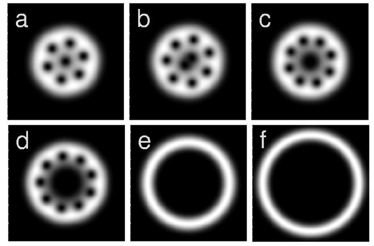
Figure 1: Density profiles of a rotating condensate at $g=80$ and $\lambda=0.5$, for (a) $\Omega=2.0$, (b) $\Omega=2.1$, (c) $\Omega=2.25$, (d) $\Omega=2.5$, (e) $\Omega=3.0$, (f) $\Omega=3.5$. The scale of each figure is $4\times 4$ in units of $d_{\perp}$.

We have also performed calculations for stronger interactions ($g=1000$). In this case one finds a vortex lattice at $\Omega=2.0$, as before [Fig. 2(a)]. However, as $\Omega$ increases, a density depression appears in the center of the condensate, with an associated increase in the core size of the central vortices [Fig. 2(b)]. At approximately $\Omega\simeq 3.3$, the density dips to zero at the center, which can be taken to be the numerical value of $\Omega_{h}$. Figure 2(c) shows a typical configuration with a central hole surrounded by two rows of vortices. As $\Omega$ increases, the inner row is absorbed by the expanding hole until, in Fig. 2(f) ($\Omega=5.0$) only one row of vortices remains. For larger $\Omega$, we find that the inner and outer radii of the condensate both increase in size, but the basic structure (a hole with a single ring of vortices) remains the same. We see no transition to the giant-vortex state up to $\Omega=7.0$, above which unfortunately the numerics become very difficult. Nevertheless, this value sets a lower bound on $\Omega_{g}$ for the transition to the giant vortex. For this angular velocity, the TF gap width and healing length from Eqs. (17) and (23) are $d\approx 1.43$ and $\xi\approx 0.144$, so that the TF approximation is well justified. Also note that the density distributions discussed here are qualitatively similar to the radial profiles found in a three-dimensional calculation of Ref. Afta03 .

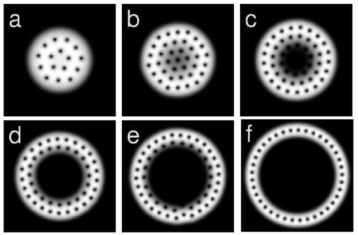
Figure 2: Density profiles of a rotating condensate at $g=1000$ and $\lambda=0.5$, for (a) $\Omega=2.0$, (b) $\Omega=3.0$, (c) $\Omega=3.5$, (d) $\Omega=4.0$, (e) $\Omega=4.5$, (f) $\Omega=5.0$, showing the stable vortice lattice configurations. The scale of each figure is $6\times 6$ in units of $d_{\perp}$.

To make a quantitative comparison of the numerical results in Fig. 2 with the analytical results, we have measured the intervortex spacing $b_{\rm meas}$ for the nearly triangular lattices in Figs. 2(a)-(d) and compared them with the predicted values for an ideal triangular lattice using the expression $b_{\rm tri}^{2}=2\pi/(\sqrt{3}\Omega)$. Table I shows that they agree very well, but the measured values $b_{\rm meas}$ decrease somewhat more slowly than would be expected for an ideal lattice at the same angular velocity.

Table 1: Comparison of numerical values for intervortex lattice spacing $b_{\rm meas}$ in a rotating condensate with $g=1000$ and $\lambda=0.5$ (obtained by direct measurements from Fig. 2) to the theoretical intervortex spacing $b_{\rm tri}$ for an ideal triangular lattice.

$\Omega$	$b_{\rm meas}$	$b_{\rm tri}$
2.0	1.32	1.35
3.0	1.08	1.10
3.5	1.01	1.02
4.0	0.97	0.95

For larger angular velocities, the vortex array is one-dimensional and the annular condensate becomes increasingly narrow. The mean radius $R_{\rm meas}$ and width $d_{\rm meas}$ can be measured from the numerical solutions by defining a reference density (in this case $|\psi|^{2}=10^{-4}$) and noting the radii at which the density is equal to this reference. Note that the inner and outer radii derived from this technique will differ from those calculated using the TF approximation, since in the latter case the density vanishes at well-defined points, while for the numerical results it does not. Nevertheless, the value of the measured mean radius is not likely to be affected too much by this detail and can be compared with the TF prediction $R_{\rm TF}$, which follows from an expression similar to Eq. (17). In addition, from $R_{\rm meas}$ and the number ${\cal N}_{a}$ of vortices in the array, we can readily calculate the intervortex spacing $b_{\rm meas}$ (Fig. 2 contains only the condensate for $\Omega=5.0$, but those for $\Omega=6.0$ and 7.0 are qualitatively similar). Finally, the measured width $d_{\rm meas}$ of the annular condensates can be compared to the TF prediction in Eq. (17). Note, however, that $d_{\rm meas}$ is affected by the numerical technique used to extract the radii, so only the $\Omega$ dependence can be checked when comparing to $d_{\rm TF}$. Table II contains these quantities. The most striking feature is that the measured intervortex spacing actually increases with increasing $\Omega$, in contrast to the $1/\sqrt{\Omega}$ dependence for an ideal triangular lattice. This behavior, which can be considered an extrapolation of that in Table I, may be a precursor of the transition to a giant vortex. The values of ${\cal N}_{a}$ found in our numerical solutions are much lower than those calculated from (15), which may reflect a non-uniform vortex density near to the edge of the condensate. In addition, Eq. (15) assumes a dense vortex array and therefore gives only a semi-quantative estimate of the number of vortices in the annulus when the array becomes one dimensional.

Table 2: Comparison of selected numerical values for a rotating condensate with $g=1000$ and $\lambda=0.5$ (obtained from Fig. 2) to some of the TF predictions. The intervortex spacing $b_{\rm meas}$ for the one-dimensional vortex arrays follows from direct measurements of the mean radius $R_{\rm meas}$ and the vortex number in the annulus ${\cal N}_{a}$.

$\Omega$	$R_{\rm meas}$	$R_{\rm TF}$	${\cal N}_{a}$	$b_{\rm meas}$	$d_{\rm meas}$	$d_{\rm TF}$
5.0	4.83	4.79	37	0.821	2.32	2.06
6.0	5.80	5.86	44	0.828	1.98	1.68
7.0	6.85	6.89	51	0.844	1.76	1.43

Figure 3 compares the $\Omega$-$g$ phase diagram resulting from this numerical analysis to the analytical TF results presented earlier. One can see that the value of $\Omega_{h}$ found in the numerical calculations is very close to the analytical result in Eq. (12). This is true not only for the value of $g=1000$ presented in Fig. 2; even for $g=80$ the agreement is very good, which is somewhat surprising since the Thomas-Fermi approximation assumed in the analytic result is expected to be less accurate. Given the difficulty in identifying the exact point at which the hole forms, the numerical value of $\Omega_{h}$ quoted here is approximate, with an error of $\pm 0.1$. In addition one can see that both the analytical and numerical results are very close to those of Kavoulakis and Baym Kavo03 . Near the horizontal axis, Fig. 3 also shows the crossover to a region where the Thomas-Fermi approximation is expected to fail, as estimated by the criterion $d^{2}\approx 10\xi^{2}$ with $d$ and $\xi$ given by Eqs. (17) and (23).

We have also calculated the energies of these vortex-lattice configurations. The numerical and analytical results will be discussed in the next section.

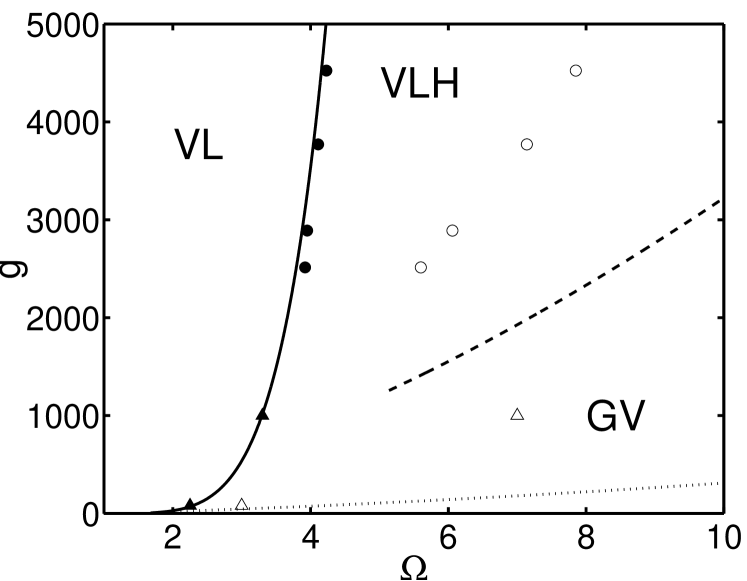
Figure 3: Phase diagram of a condensate rotating with angular velocity $\Omega$ versus interaction strength $g$, with $\lambda=0.5$, where the solid line is the critical frequency $\Omega_{h}$ [Eq. (12)] derived from our TF analysis. Going from left to right, the first state (denoted VL) is a vortex lattice without a hole, while above $\Omega_{h}$ (solid line) a hole appears (denoted VLH). Then, for $\Omega>\Omega_{g}$ (dashed line) the TF analysis predicts a giant vortex state (denoted GV). In addition, the dotted line indicates the crossover region where the TF approximation fails [defined here by the somewhat arbitrary criterion $d^{2}\approx 10\xi^{2}$, where $d$ and $\xi$ are given by Eqs. (17) and (23)]. For comparision we also show the results of Kavoulakis and Baym Kavo03 , where the filled and open circles represent $\Omega_{h}$ and $\Omega_{g}$ respectively. Finally, our numerical results for these quantities are plotted as filled and open triangles.

V Irrotational flow in annular region (“giant vortex”)

The vortex array considered in Sec. III has the uniform vortex density $\Omega/\pi$ in dimensionless oscillator units, which defines an effective vortex radius $l=1/\sqrt{\Omega}$. In any rotating superfluid, this quantity decreases with increasing angular velocity. The new feature of the present system is that the geometry itself also depends on $\Omega$. In particular, Eq. (18) shows that the width of the annulus decreases proportional to $1/\Omega$ and eventually becomes comparable with the intervortex distance $\approx 2l$. Near this critical angular velocity, the vortex array first becomes one-dimensional and then should disappear in a transition (perhaps a crossover) to pure irrotational flow, as seen in the numerical simulations of Sec. IV and Ref. Kasa02 and studied in an approximate TF theory in Ref. Kavo03 .

V.1 Pure irrotational flow

To study this behavior in detail, it is first necessary to first consider the case of pure irrotational flow, when $\psi(\bm{r})=e^{i\nu\phi}|\psi(r)|$ with $\nu$ the quantum of circulation (and $\nu$ is the angular momentum in units of $\hbar$). The resulting velocity is azimuthal with $v_{\rm irr}(r)=\nu/r$. Since $\nu$ will be large, it can be treated as a continuous variable, ignoring the discrete transitions between adjacent large integral values. The TF density is now given by

$$g|\psi|^{2}=\tilde{\mu}-U(r^{2}),$$ (27)

where $\tilde{\mu}=\mu+\Omega\nu$ is a constant Fisc03 ; Kavo03 and

$$U(x)=\frac{1}{2}\left(\frac{\nu^{2}}{x}+x+\lambda x^{2}\right)$$ (28)

can be considered an effective potential that combines the centrifugal barrier and the original trap potential (here, $x=r^{2}$). This function $U(x)$ has a single minimum at $x_{0}$ determined by $U^{\prime}(x_{0})=0$, so that $x_{0}$ is also the position of the local maximum in the TF density. The density vanishes at the two classical turning points $x_{1}=R_{1}^{2}$ and $x_{2}=R_{2}^{2}$, determined by the condition

$$U(x_{i})=\tilde{\mu},$$ (29)

where $x_{1}<x_{0}<x_{2}$.

The normalization condition can be written

$$g=\pi\int_{x_{1}}^{x_{2}}dx\,\left[\tilde{\mu}-U(x)\right],$$ (30)

along with the free energy per particle

$$\frac{gF}{N}=-\frac{1}{2}\pi\int_{x_{1}}^{x_{2}}dx\,\left[\tilde{\mu}-U(x)\right]^{2}.$$ (31)

Here, the physical quantities $N(\mu,\nu,\Omega)$ and $F(\mu,\nu,\Omega)$ depend explicitly on the chemical potential $\mu$ and the angular velocity $\Omega$; equivalently, the normalization condition (30) can also be obtained from the thermodynamic derivative $N=-\partial F/\partial\mu$. The equilibrium value of the circulation $\nu$, which is an additional parameter in the calculation, follows by minimizing the free energy, $\partial F/\partial\nu=0$, yielding Kavo03

$$g\,\Omega=\nu\pi\int_{x_{1}}^{x_{2}}\frac{dx}{x}\left[\tilde{\mu}-U(x)\right].$$ (32)

For a given $N$ and $\Omega$, Eqs. (29), (30) and (32) must be evaluated to find the energy $E^{\prime}(N,\Omega)$ in the rotating frame. Comparison with the corresponding quantity for the condensate containing a one-dimensional vortex array then determines the phase diagram. In Ref. Kavo03 , this procedure was carried out numerically, which does not emphasize the relevant parameters needed for a physical interpretation. Instead, we recall that the annulus expands radially and becomes increasingly narrow for large $\Omega$, as seen in Eqs. (18) and (19). Thus an expansion in the small parameter $d/R\sim[\lambda^{2}\,g/(4\pi)]^{1/3}\Omega^{-2}$ characterizes the irrotational state in the relevant limit of rapid rotation.

The minimum $x_{0}$ of the potential $U(x)$ in Eq. (28) satisfies the cubic equation

$$2\lambda x_{0}^{3}+x_{0}^{2}=\nu^{2},$$ (33)

which makes a direct analysis quite intricate. Instead, the large value of $x_{0}\approx R^{2}$ relative to $x_{2}-x_{1}\approx 2Rd$ makes it natural to expand $U(x)$ around $x_{0}$, and it is necessary to include corrections through order $(x-x_{0})^{4}$. To make this procedure precise, let $x-x_{0}=x_{0}\delta$, where $|\delta|\ll 1$, so that the inner and outer boundaries are given by $x_{i}=x_{0}(1+\delta_{i})$. In addition, let

$$\tilde{\mu}-U(x_{0})=\frac{1}{2}(3\lambda x_{0}^{2}+x_{0})\delta_{0}^{2},$$ (34)

which defines $\delta_{0}$ in terms of the other parameters. It is not difficult to determine $\delta_{1}$ and $\delta_{2}$ as series in powers of $\delta_{0}$, and it is sufficient to keep terms of order $\delta_{0}^{3}$. In this way, Eqs. (30) and (31) reduce to integrals of the form $\int_{\delta_{1}}^{\delta_{2}}d\delta\,\cdots$, where $\cdots$ denotes a function that is readily expanded in powers of $\delta$.

A lengthy analysis eventually leads to useful and physical expressions. For example, the ratio of Eqs. (30) and (32) yields the somewhat implicit expression for the quantum of circulation

$$\nu\approx\Omega x_{0}\left(1+\frac{\delta_{0}^{2}}{30\lambda x_{0}}\right).$$ (35)

As expected, the leading term here is simply the quantum number associated with the angular momentum $\Omega x_{0}=\Omega R^{2}$ of a narrow annulus, and the term of order $\delta_{0}^{2}$ arises from the small TF corrections.

The next step is to solve the cubic equation (33) for $x_{0}$ by expanding it for large values of $(\nu^{2}/2\lambda)^{1/3}$. The resulting power series for $x_{0}$ can be combined with (35) to give the mean squared radius

$$x_{0}\approx\frac{\Omega^{2}-1}{2\lambda}+\frac{\delta_{0}^{2}}{15\lambda},$$ (36)

and the associated circulation

$$\nu\approx\frac{\Omega\,(\Omega^{2}-1)}{2\lambda}+\frac{\Omega\,\delta_{0}^{2}}{10\lambda}.$$ (37)

Note that the leading term for $x_{0}$ reproduces (13) for the mean squared radius of an annulus with a uniform vortex array and the leading term for $\nu$ reproduces the angular momentum (21) for an annulus with a uniform vortex array; in both cases, the corrections involve the small parameter $\delta_{0}^{2}$. A combination of Eqs. (34) and (37) then gives the chemical potential

$$\mu\approx-\frac{(\Omega^{2}-1)^{2}}{8\lambda}+\frac{3\Omega^{4}\delta_{0}^{2}}{8\lambda}.$$ (38)

The remaining step is to determine the small parameter $\delta_{0}$ from Eqs. (30) and (36), leading to

$$\delta_{0}\approx\frac{2\sqrt{\lambda}}{\Omega^{2}}\,\left(\frac{\sqrt{\lambda}\,g}{2\pi}\right)^{1/3}.$$ (39)

Since $\delta_{0}$ is small, this result requires $[\lambda^{2}g/(4\pi)]^{1/3}\ll\Omega^{2}$, which ensures that $d/R\ll 1$. These relations readily provide the inner and outer squared radii $R_{1}^{2}=x_{0}+x_{0}\delta_{1}$ and $R_{2}^{2}=x_{0}+x_{0}\delta_{2}$. To leading order, the mean squared radius is $x_{0}$ and the width is given by $d^{2}\approx x_{0}\delta_{0}^{2}\approx(2/\Omega^{2})[\sqrt{\lambda}\,g/(2\pi)]^{2/3}$. In more detail,

$$R_{2}^{2}+R_{1}^{2} \approx \frac{\Omega^{2}-1}{\lambda}+\frac{4}{3\Omega^{2}}\left(\frac{\sqrt{\lambda}\,g}{2\pi}\right)^{2/3},$$ (40)

$$R_{2}^{2}-R_{1}^{2} \approx \frac{2}{\sqrt{\lambda}}\left(\frac{\sqrt{\lambda}\,g}{2\pi}\right)^{1/3}.$$ (41)

Comparison with Eqs. (13) and (15) shows that the mean squared radius here slightly exceeds that for the annulus with a uniform vortex array, whereas the width here is smaller by a factor $3^{-1/3}$.

Substitution into Eq. (38) expresses the chemical potential for the irrotational giant vortex in terms of the appropriate variables $N$ and $\Omega$

$$\mu_{\rm irr}\approx-\frac{(\Omega^{2}-1)^{2}}{8\lambda}+\frac{3}{2}\left(\frac{\sqrt{\lambda}\,g}{2\pi}\right)^{2/3}.$$ (42)

Integration of the thermodynamic relation (3) then yields the energy in the rotating frame

$$E_{\rm irr}^{\prime}\approx-\frac{N}{8\lambda}\left(\Omega^{2}-1\right)^{2}+\frac{9N}{10}\left(\frac{\sqrt{\lambda}\,g}{2\pi}\right)^{2/3}.$$ (43)

It is not surprising that the energy (20) for an annulus with uniform and continuous vorticity $2\bm{\Omega}$ is lower than (43) for pure irrotational flow. Indeed, a fluid in solid-body rotation necessarily has a lower energy in the rotating frame than other velocity distributions, which follows by minimizing the functional $E^{\prime}[{\bm{v}}]=\int dV\rho\left(\frac{1}{2}v^{2}-\bm{\Omega\cdot r\times v}\right)$ with respect to $\bm{v}(\bm{r})$.

A good test of the analytical TF results is to compare the TF energy per particle to the values extracted directly from our numerical calculations, as is shown in Fig. 4 for $g=1000$ and $\lambda=0.5$. The open circles are the energies corresponding to the vortex-lattice states calculated numerically as shown in Fig. 2. These are compared to the analytical result from Eq. (20), which was derived assuming a Thomas-Fermi profile and uniform vorticity. We find a small but significant discrepancy between them, where the analytical result is smaller by typically $\Delta E\sim 6$. This is not surprising because (20) assumes solid-body rotation which provides a lower bound to the energy. In detail, we attribute this discrepancy to the energy associated with the vortex cores, which will give a correction to the analytical result due to the irrotational flow and density dip near to each vortex.

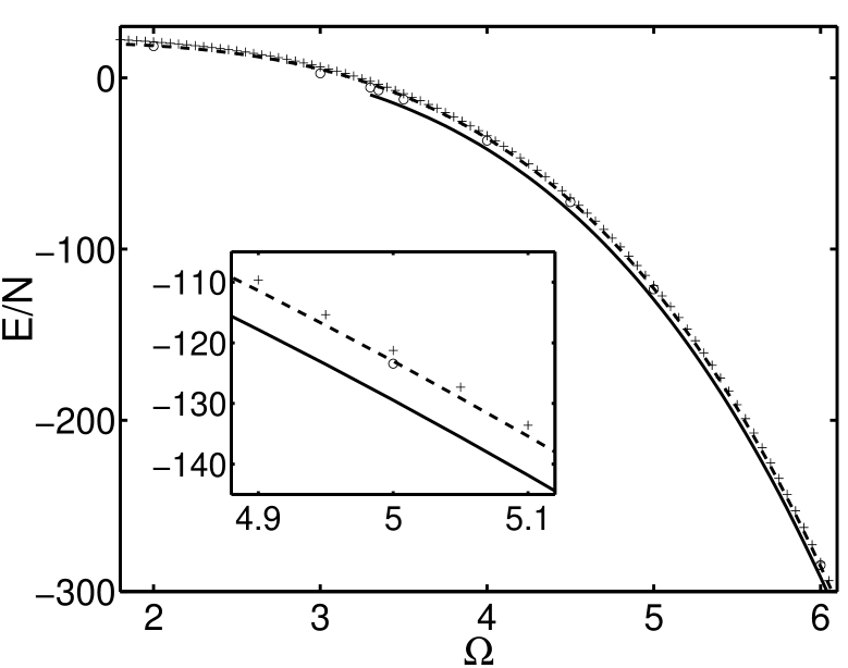
Figure 4: Energy per particle vs. rotation rate $\Omega$, where our numerical results are presented as open circles (vortex-lattice state) and crosses (giant-vortex state). For comparision, the analytical results are plotted as a solid line (Thomas-Fermi vortex lattice with hole) and a dashed line (giant vortex). The inset shows the energies in a small region of the graph around $\Omega=5$. The parameters used here are $g=1000$ and $\lambda=0.5$.

We also calculate the energy of the giant-vortex state by numerically solving Eq. (26) with $\Omega=0$ and replacing $V_{\rm tr}$ with $V_{\rm tr}+\nu^{2}/(2r^{2})$, where $\nu$ is the quantum of circulation of the macroscopic flow. We calculate the energy $E_{\nu}$ for each $\nu$, which in the rotating frame becomes $E_{\nu}^{\prime}=E_{\nu}-\nu\Omega$. The energy as a function of $\Omega$ is then the minimum possible $E_{\nu}^{\prime}$ for that particular $\Omega$, which also fixes the relevant $\nu$. The density profiles of the giant-vortex states corresponding to the same angular velocities as in Fig. 2 are plotted in Fig. 5, while the energies are plotted as the crosses in Fig. 4. Note that the energy of the vortex lattice is always lower than the corresponding giant vortex for the range of $\Omega$ covered, which reconfirms the conclusion from Fig. 2 that no transition occurs to the giant-vortex state since it is energetically unfavorable to do so. It is also in contrast to the results at $g=80$, which demonstrate that the giant vortex state can indeed become energetically favorable at high angular velocities (as seen in Fig. 1). We also compare our results to the analytical energy of the giant vortex Eq. (43) and find quite good agreement for larger values of $\Omega$, with the analytical result being smaller by around $\Delta E\sim 2$.

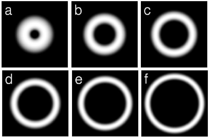
Figure 5: Density profiles of a rotating condensate at $g=1000$ and $\lambda=0.5$, showing the giant-vortex states corresponding to the angular velocities in Fig. 2: (a) $\Omega=2.0$, (b) $\Omega=3.0$, (c) $\Omega=3.5$, (d) $\Omega=4.0$, (e) $\Omega=4.5$, (f) $\Omega=5.0$. The scale of each figure is $6\times 6$ in units of $d_{\perp}$.

V.2 Transition to a giant vortex

The assumption of uniform vorticity is reasonable as long as the intervortex distance is much smaller than any of the dimensions of the annulus. It fails when the discrete character of the quantized vortex lines becomes significant, in particular, when the width $d$ of the annulus becomes comparable to the intervortex separation $b\sim 2l=2/\sqrt{\Omega}$.

As background, it is instructive to review the analogous transition in rotating superfluid ⁴He in an annulus. Here, the width $d$ is fixed by the geometry of the container, and vortices first appear with increasing $\Omega$ when $b$ is of order $d$. To be more precise, the irrotational flow in an annulus has the characteristic feature that the velocity $v_{\rm irr}=\nu/r$ decreases with increasing $r$, whereas the preferred solid-body flow $v_{\rm sb}=\Omega r$ increases. For a fixed gap width, this discrepancy grows as $\Omega$ increases, and it eventually becomes favorable to insert a one-dimensional array of quantized vortices at the midpoint of the annulus. On average, the circulating velocity around each core combines with the overall irrotational flow to mimic more closely $\bm{v}_{\rm sb}$, thus lowering the energy in the rotating frame. A detailed analysis of the free energy of the various relevant states  Fett67 predicted that a one-dimensional vortex array appears with increasing $\Omega$ at a (dimensional) critical angular velocity $\Omega_{0}=(\kappa/\pi d^{2})\ln(d/\xi)$, where $d$ is the width of the annular gap and $\xi$ is the vortex core radius. The theory indicated that the vortices appear one by one in a very narrow interval of $\Omega$, rapidly building up a one-dimensional vortex array in the center of the gap. Experiments on superfluid ⁴He using second-sound attenuation verified this predicted critical angular velocity in considerable detail Bend67 (including the location at the midpoint of the gap).

In the present case of a rotating annular condensate, the width $d$ decreases like $1/\Omega$, which is faster than the decrease of the intervortex spacing. Hence the transition here is expected to occur in the reverse order, with the irrotational giant vortex appearing for large $\Omega$. The relevant comparison state is a one-dimensional vortex array in addition to the irrotational flow, as seen in Fig. 2(f). For a preliminary estimate, it is convenient to study only the case of a single vortex located at the midpoint of the gap combined with macroscopic circulation. The analysis is lengthy and will not be given here because the resulting critical angular velocity does not agree well with the numerical work. Thus it suffices merely to state that the transition from one vortex with irrotational flow to the pure irrotational flow is predicted to occur at a critical angular velocity

$$\Omega_{g}\approx\frac{1}{\ln(d^{2}/\xi^{2})}\left(\frac{\sqrt{\lambda}\,g}{2\pi}\right)^{2/3},$$ (44)

as the angular velocity increases.

Figure 3 also compares the critical angular velocity $\Omega_{g}$ for the transition from the vortex lattice to the giant-vortex state. First, we see that our analytical $\Omega_{g}$ is much larger than that of Ref. Kavo03 (open circles). In addition, our numerical result (open triangle) is much larger than even our analytical prediction (in Fig. 3 we plot the lower bound on $\Omega_{g}$ in the case of $g=1000$ since the numerical methods place constraints on using higher rotations, as discussed above). Note that we plot (44) only for large $g$, since logarithmic accuracy is expected to be poor for small $g$. Even for $\Omega$ larger than $\Omega_{g}$, the lowest energy solution of the GP equation does not correspond to a giant vortex, which suggests that for these values of $\Omega$ the giant vortex is stable against the formation of a single vortex, but is unstable against the formation of an array of vortices (see Fig. 2).

VI Discussion

This work has considered a two-dimensional rapidly rotating Bose-Einstein condensate in a radial trap with both quadratic and quartic confining components, which allows the external rotation $\Omega$ to exceed the harmonic trap frequency $\omega_{\perp}$. Both an analytical Thomas-Fermi description and a full numerical study of the Gross-Pitaevskii equation show the formation of a central hole at essentially the same critical angular velocity $\Omega_{h}$ (the analytical value apparently remains quite accurate even for small values of the coupling constant $g=4\pi Na/Z$ where the Thomas-Fermi approximation is less valid). For larger angular velocities, the numerical work for $g=80$ indicates a transition to a pure irrotational state (a giant vortex), but our approximate analytical model predicts too small a value for this transition.

Experimental work at the École Normale Supérieure, Paris Bret04 ; Stoc04 created a quartic confinement with a blue-detuned Gaussian laser directed along the axial direction. For their trap, the nonrotating condensate was cigar shaped, and the strength of the quartic admixture was $\lambda\approx 10^{-3}$. For dimensionless rotation speed $\Omega\sim 1$, the condensate was nearly spherical, and it remained stable for $\Omega\lesssim 1.05$. Near the upper limit, the condensate exhibited a definite local minimum in the central density, confirming the general features of our TF analysis. Throughout the stable range of $\Omega$, the measured shape of the condensate was fit to the TF prediction, which served as a direct determination of $\Omega$. They also used surface-wave spectroscopy Zamb98 ; Cozz03 to provide an independent measure of the angular velocity (even though the visible number of vortices appeared to be too small for $\Omega\geq 1$).

These experiments are very puzzling when compared to the previous numerical studies Kasa02 ; Afta03 , to previous analytical studies Kavo03 and to the present work. Why do the experiments fail to reach higher angular velocities, when the simulations readily reach the regime when the condensate becomes annular? One possible source of the discrepancy is that the experimental condensate is definitely three-dimensional, whereas the simulations are two-dimensional (apart from Afta03 ). It is notable that even the experimental papers Bret04 ; Stoc04 suggest repeating the experiments with a condensate that is tightly confined in the $z$ direction. In addition, the low temperature of the experiments eliminates most dissipative processes that can equilibrate the system. This feature may make it difficult for the condensate to acquire more angular momentum as $\Omega$ increases. In contrast, the numerical simulations work in imaginary time for a given $\Omega$, which leads to a state that is at least a local minimum in the energy.

Another different question concerns the transition to the giant vortex. Our numerical simulations indicate that this transition occurs well beyond our analytical estimate $\Omega_{g}$ in Eq. (44). This estimate is obtained by comparing the energy of the irrotational giant vortex with a similar irrotational state containing one additional quantized vortex at the midpoint of the annulus. Based on the numerical simulations [especially Fig. 2(f)], it seems probable that adding more quantized vortices in a one-dimensional ring and/or allowing the radius of the ring to vary would lower the energy of this state relative to the irrotational state, because the specific choice of one vortex at the midpoint seems somewhat arbitrary for a dilute trapped condensate. For superfluid ⁴He in a rotating annulus, the image vortices raise the energy if a vortex approaches either wall, but such an effect is absent in the present case. If so, such an improved analysis would increase the estimated critical angular velocity for the transition to a giant vortex. It is also conceivable that the mean radius of the one-dimensional vortex array simply shrinks inside the inner TF radius $R_{1}$. This latter situation would suggest a crossover instead of a sharp transition, because the actual condensate necessarily extends into the classically forbidden region. These questions remain for future investigation.

- (1) M.R. Matthews, B.P. Anderson, P.C. Haljan, D.S. Hall, C.E. Wieman, and E.A. Cornell, Phys. Rev. Lett. 83, 2498 (1999).
- (2) K.W. Madison, F. Chevy, W. Wohlleben, and J. Dalibard, Phys. Rev. Lett. 84, 806 (2000).
- (3) J.R. Abo-Shaeer, C. Raman, J.M. Vogels, and W. Ketterle, Science 292, 476 (2001).
- (4) C. Raman, J.R. Abo-Shaeer, J.M. Vogels, K. Xu, and W. Ketterle, Phys. Rev. Lett. 87, 210402 (2001).
- (5) P.C. Haljan, I. Coddington, P. Engels, and E.A. Cornell, Phys. Rev. Lett. 87, 210403 (2001).
- (6) P. Engels, I. Coddington, P.C. Haljan, and E.A. Cornell, Phys. Rev. Lett. 89, 100403 (2002).
- (7) A.L. Fetter, Phys. Rev. A 64, 063608 (2001).
- (8) T.-L. Ho, Phys. Rev. Lett. 87, 060403 (2001).
- (9) V. Schweikhard, I. Coddington, P. Engels, V.P. Mogendorff, and E.A. Cornell, Phys. Rev. Lett. 92, 040404 (2004).
- (10) I. Coddington, P.C. Haljan, P. Engels, V. Schweikhard, S. Tung, and E.A. Cornell, cond-mat/0405240
- (11) E. Lundh, Phys. Rev. A 65, 043604 (2002).
- (12) V. Bretin, S. Stock, Y. Seurin, and J. Dalibard, Phys. Rev. Lett. 92, 050403 (2004).
- (13) S. Stock, V. Bretin, F. Chevy, and J. Dalibard, Europhys. Lett. 65, 594 (2004).
- (14) K. Kasamatsu, M. Tsubota, and M. Ueda, Phys. Rev. A 66, 053606 (2002).
- (15) G.M. Kavoulakis and G. Baym, New J. Phys. 5, 51.1 (2003).
- (16) A.D. Jackson, G.M. Kavoulakis, and E. Lundh, Phys. Rev. A 69, 053619 (2004).
- (17) U.R. Fischer and G. Baym, Phys. Rev. Lett. 90, 140402 (2003).
- (18) A.L. Fetter, Phys. Rev. 153, 285 (1967).
- (19) G. Baym and C.J. Pethick, Phys. Rev. A 69, 043619 (2004).
- (20) A. Aftalion and I. Danaila, Phys. Rev. A 69, 033608 (2004).
- (21) To propagate Eq. (26), we use a Fast Fourier Transform method, where the partial derivatives (in both the kinetic and angular momentum terms) are treated by Fourier transforming into momentum space. This method involves discretizing the wavefunction using a grid, where we typically use a grid spacing of .
- (22) P.J. Bendt and R.J. Donnelly, Phys. Rev. Lett. 19, 214 (1967).
- (23) F. Zambelli and S. Stringari, Phys. Rev. Lett. 81, 1754 (1998).
- (24) M. Cozzini and S. Stringari, Phys. Rev. A 67, 041602(R) (2003).