Simple theoretical tools for low dimension Bose gases

Abstract

We first consider an exactly solvable classical field model to understand the coherence properties and the density fluctuations of a one-dimensional (1D) weakly interacting degenerate Bose gas with repulsive interactions at temperatures larger than the chemical potential. In a second part, using a lattice model for the quantum field, we explain how to carefully generalize the usual Bogoliubov approach to study a degenerate and weakly interacting Bose gas in 1D, 2D or 3D in the regime of weak density fluctuations. In the last part, using the mapping to an ideal Fermi gas in second quantized formalism, we calculate and discuss physically the density fluctuations and the coherence properties of a gas of impenetrable bosons in 1D.

1 A classical field model for the 1D weakly interacting Bose gas

1.1 Reminder: quantum theory for the ideal Bose gas

1.1.1 Second quantized formalism

We consider the case of spinless, non-relativistic bosons of mass $m$ moving in a space of spatial coordinates of dimension $d$ and stored either in a trapping potential $U(\mathbf{r})$ or in a cubic box of size $L$ with periodic boundary conditions. In this subsection the bosons are not interacting. The grand canonical Hamiltonian has then the following expression in second quantized formalism:

$$\hat{H}=\int d\mathbf{r}\,\hat{\psi}^{\dagger}(\mathbf{r})(h_{0}-\mu)\hat{\psi}(\mathbf{r}).$$ (1)

$\mu$ is the chemical potential, and the differential operator $h_{0}$ includes the kinetic energy operator and the trapping potential $U(\mathbf{r})$:

$$h_{0}=-\frac{\hbar^{2}}{2m}\Delta+U(\mathbf{r})$$ (2)

where $\Delta$ is the Laplacian operator in dimension $d$. Note that $U\equiv 0$ in the spatially homogeneous case of a cubic box. The field operator $\hat{\psi}(\mathbf{r})$ annihilates a boson in point $\mathbf{r}$ and obeys the usual bosonic commutation relations:

$$[\hat{\psi}(\mathbf{r}),\hat{\psi}(\mathbf{r}^{\prime})]=0,$$ (3)

$$[\hat{\psi}(\mathbf{r}),\hat{\psi}^{\dagger}(\mathbf{r}^{\prime})]=\delta(\mathbf{r}-\mathbf{r}^{\prime}).$$ (4)

It is convenient to expand the field operator on the orthonormal basis of the eigenmodes $\phi_{\alpha}(\mathbf{r})$ of $h_{0}$ with eigenenergy $\epsilon_{\alpha}$:

$${\hat{\psi}}(\mathbf{r})=\sum_{\alpha}\phi_{\alpha}(\mathbf{r})\hat{a}_{\alpha}$$ (5)

$$\left[-\frac{\hbar^{2}}{2m}\Delta+U(\mathbf{r})\right]\phi_{\alpha}(\mathbf{r})=\epsilon_{\alpha}\phi_{\alpha}(\mathbf{r})$$ (6)

where $\hat{a}_{\alpha}$ annihilates a particle in mode $\phi_{\alpha}$. The grand canonical Hamiltonian is then a sum of decoupled harmonic oscillators:

$$\hat{H}=\sum_{\alpha}(\epsilon_{\alpha}-\mu)\hat{a}_{\alpha}^{\dagger}\hat{a}_{\alpha}.$$ (7)

1.1.2 In thermal equilibrium

We consider for convenience that the gas is in thermal equilibrium in the grand canonical ensemble so that the density operator of the system reads

$$\hat{\rho}=\Xi^{-1}e^{-\beta\hat{H}}$$ (8)

where $\beta=(k_{B}T)^{-1}$ is inversely proportional to the temperature $T$. As the canonical ensemble is more realistic, since no reservoir of particles is present in usual experiments, one has to check for each particular case at hand that the two ensembles are almost equivalent, a point that we will address in 1.1.4.

For the ideal Bose gas the density operator is a Gaussian in the field components so that Wick’s theorem, an elementary proof of which is given in the appendix 4, allows to express the expectation value

$$\langle\hat{O}\rangle\equiv\mbox{Tr}[\hat{O}\hat{\rho}]$$ (9)

of an arbitrary observable $\hat{O}$ in terms of the mean occupation numbers of the eigenmodes:

$$n_{\alpha}\equiv\langle\hat{a}_{\alpha}^{\dagger}\hat{a}_{\alpha}\rangle.$$ (10)

These occupation numbers are given by the Bose formula, also rederived in the appendix 4:

$$n_{\alpha}=\frac{1}{e^{\beta(\epsilon_{\alpha}-\mu})-1}.$$ (11)

Assuming here for convenience that the ground state energy of $h_{0}$ vanishes, which amounts to shifting the chemical potential, we see that the positivity of $n_{\alpha}$ imposes the following range of variation of $\mu$:

$$-\infty<\mu<0.$$ (12)

In what follows one considers a temperature regime significantly different from the zero temperature case, that is one assumes that there is a large number of eigenmodes of energy less than $k_{B}T$. In the spatially homogeneous case this implies that the size of the box is larger than the thermal de Broglie wavelength:

$$L\gg\lambda.$$ (13)

One recalls the various regimes then encountered for $\mu$ increasing from $-\infty$ to zero, in the present case of a non-degenerate ground mode:

• $|\mu|\gg k_{B}T$: non-degenerate regime. All the occupation numbers are much smaller than unity and are well approximated by the Boltzmann formula:

  $$n_{\alpha}\simeq e^{-\beta(\epsilon_{\alpha}-\mu})\ll 1.$$ (14)

  Summing this expression over $\alpha$ relates the chemical potential to the mean number $N$ of particles. In the case of the cubic box, and if one replaces the sum by an integral, as allowed by condition (13), this leads to

  $$e^{\beta\mu}\simeq\rho\lambda^{d}$$ (15)

  where $\rho=N/L^{d}$ is the mean density and $\lambda$ is the thermal de Broglie wavelength

  $$\lambda^{2}=\frac{2\pi\hbar^{2}}{mk_{B}T}$$ (16)

  so that we recover the condition for a non-degenerate regime

  $$\rho\lambda^{d}\ll 1.$$ (17)

• degenerate regime: $|\mu|\ll k_{B}T$ so that the ground mode of the gas has a large occupation number:

  $$n_{0}\simeq\frac{k_{B}T}{|\mu|}\gg 1$$ (18)

  where we have expanded the exponential in the Bose law to first order in its argument. In this case several modes have a large occupation number, as soon as $|\mu|\ll k_{B}T$, because condition (13) holds.

• the ground mode is more populated than any other mode: this regime is reached when the ground mode is more populated that the first excited mode:

  $$n_{0}\simeq\frac{k_{B}T}{|\mu|}\gg n_{1}\simeq\frac{k_{B}T}{|\epsilon_{1}-\mu|}$$ (19)

  which results in

  $$|\mu|\ll\epsilon_{1}.$$ (20)

  It is the right time to recall the phenomenon of saturation of the total occupation of the excited modes, a key consequence of the Bose law: for a given temperature the maximal value of the excited modes population is

  $$N^{\prime}\equiv\sum_{\alpha\neq 0}n_{\alpha}<N^{\prime}_{\rm max}\equiv\sum_{\alpha\neq 0}\frac{1}{e^{\beta\epsilon_{\alpha}}-1}$$ (21)

  where one used the fact that each occupation number, being an increasing function of the chemical potential, is bounded from above by its value for $\mu=0$. An important consequence of (20) is that the saturation of the excited modes population is quasi reached, as $\mu$ is negligible compared to all $\epsilon_{\alpha}$ in the sum defining $N^{\prime}_{\rm max}$:

  $$N^{\prime}\simeq N^{\prime}_{\rm max}.$$ (22)

• Bose-Einstein condensation: the ground mode has an occupation number on the order of the total population of the excited levels. One has then

  $$n_{0}\sim N^{\prime}_{\rm max}.$$ (23)

  One recovers in particular the condition to reach Bose-Einstein condensation applicable for a finite size system, that is in the absence of thermodynamical limit [1],

  $$N>N^{\prime}_{\rm max}$$ (24)

  and the typical value of the chemical potential when a clear condensate is formed, assuming $n_{0}\sim N$ [2]:

  $$|\mu|\sim\frac{k_{B}T}{N}.$$ (25)

1.1.3 3D vs 1D in the thermodynamical limit

We estimate the value of $N^{\prime}_{\rm max}$ in a box of length much larger than the thermal de Broglie wavelength $\lambda$:

$$N^{\prime}_{\rm max}=\sum_{\mathbf{k}\neq\mathbf{0}}\frac{1}{\exp(\beta\hbar^{2}k^{2}/2m)-1}$$ (26)

where the components of the wavevector $\mathbf{k}$ are integer multiple of $2\pi/L$.

In 3D, the condition $L\gg\lambda$ allows to approximate the sum by an integral:

$$N^{\prime}_{\rm max}\simeq\zeta(3/2)\left(\frac{L}{\lambda}\right)^{3}$$ (27)

where $\zeta$ is the Riemann Zeta function. One finds that the contribution to the integral is indeed dominated by wavevectors such that $\hbar^{2}k^{2}/2m\sim k_{B}T$ since the density of states cuts the low $k$ contribution and the Bose law cuts the high $k$ contribution. So in 3D in the thermodynamic limit, the gas is essential either in the non-degenerate regime or in the Bose condensed regime.

In 1D one cannot replace the sum over $k$ by an integral without getting an infrared divergent result for $N^{\prime}_{\rm max}$: this is an indication that the low $k$ dominate. The proper approximation to get the leading order contribution in $L/\lambda$ is to replace the Bose law by its low $k$ behaviour:

$$N^{\prime}_{\rm max}\simeq\sum_{k\neq 0}\frac{k_{B}T}{\hbar^{2}k^{2}/2m}=\frac{\pi}{3}\frac{L^{2}}{\lambda^{2}}$$ (28)

where we used $\sum_{n=1}^{+\infty}1/n^{2}=\pi^{2}/6$. So in 1D in the thermodynamic limit, one can reach an arbitrarily high degeneracy $\rho\lambda$ without forming a Bose-Einstein condensate.

1.1.4 Correlation functions of the 1D Bose gas in the thermodynamic limit

The first order correlation function of the field operator $\hat{\psi}$ is defined in 1D as

$$g_{1}(z)\equiv\langle\hat{\psi}^{\dagger}(z)\hat{\psi}(0)\rangle.$$ (29)

It allows to determine the coherence length of the gas. In a 1D box, $g_{1}$ is the Fourier transform of the momentum distribution:

$$g_{1}(z)=\frac{1}{L}\sum_{k}n_{k}e^{ikz}\rightarrow\int\frac{dk}{2\pi}n_{k}e^{ikz}$$ (30)

where $\rightarrow$ corresponds to the thermodynamic limit. In the non-degenerate regime the momentum distribution reduces to the Boltzmann distribution so that $g_{1}$ is a Gaussian:

$$g_{1}(z)\simeq\rho e^{-2\pi z^{2}/\lambda^{2}}.$$ (31)

In the degenerate regime, where $|\mu|\ll k_{B}T$, we replace the Bose law by its low energy approximation, as we did in the calculation of $N^{\prime}_{\rm max}$, which results in a Lorentzian approximation to the momentum distribution:

$$n_{k}\simeq\frac{k_{B}T}{|\mu|+\hbar^{2}k^{2}/2m}.$$ (32)

After integration over $k$ one obtains the equation of state of the gas:

$$\rho\lambda=\left(\frac{\pi k_{B}T}{|\mu|}\right)^{1/2}$$ (33)

and after Fourier transform, one obtains an exponential function for $g_{1}$:

$$g_{1}(z)\simeq\rho e^{-|z|/l_{c}}$$ (34)

with the coherence length

$$l_{c}=\frac{\rho\lambda^{2}}{2\pi}\gg\lambda.$$ (35)

Note that in 3D, when a Bose-Einstein condensate is present, $g_{1}$ tends at infinity to the condensate density $\rho_{0}$.

The second order correlation function of the field to be considered here is

$$g_{2}(z)=\langle\hat{\psi}^{\dagger}(z)\hat{\psi}^{\dagger}(0)\hat{\psi}(0)\hat{\psi}(z)\rangle.$$ (36)

Note that it is simply the spatial correlation function of the field intensity (that is the density) for $z\neq 0$. It is also proportional to the probability density, when measuring the positions of the particles, of detecting the first particle in $0$ and the second one in $z$, as is most apparent in first quantized form

$$g_{2}(z)=\sum_{i\neq j}\langle\delta(\hat{z}_{j}-z)\delta(\hat{z_{i}})\rangle$$ (37)

where $\hat{z}_{i}$ is the operator giving the position of particle $i$ along $z$.

For an ideal Bose gas at thermal equilibrium in the grand canonical ensemble, the second order correlation function is readily expressed in terms of $g_{1}$ through Wick’s theorem:

$$g_{2}(z)=\rho^{2}+g_{1}^{2}(z)$$ (38)

where we used the fact that $g_{1}$ is real. This identity illustrates the phenomenon of bosonic bunching in real space: $g_{2}$ is maximum in $z=0$ where it reaches twice its asymptotic value $\rho^{2}$. This implies strong density fluctuations correlated over a spatial scale on the order of the coherent length $l_{c}$, a very negative fact from the atom laser perspective.

What happens in 3D? The same identity for $g_{2}$ holds, as a consequence of Wick’s theorem. When a condensate is present, one then finds also large density fluctuations at an arbitrarily large scale: $g_{2}(+\infty)=\rho^{2}+\rho_{0}^{2}>\rho^{2}$. Fortunately, this prediction is not correct physically and is an artifact of the anomalously large fluctuations of the number of condensate particles in the grand canonical ensemble for an ideal Bose gas. Wick’s theorem implies

$$\langle a_{0}^{\dagger 2}a_{0}^{2}\rangle=2n_{0}^{2}$$ (39)

where $a_{0}$ annihilates one particle in the condensate mode, so that the standard deviation of the number of condensate particles is predicted to be equal to its mean value $n_{0}$, which is not correct physically! As a consequence the fluctuations of the total number of particles $N$ becomes also anomalously large, $\Delta N\sim\langle N\rangle$, and the equivalence between the grand canonical ensemble and the canonical ensemble is lost. This problem is well known for the calculation of the fluctuations of the Bose condensed ideal Bose gas [3]. An easy way to avoid this problem is to use the canonical ensemble, plus a number conserving Bogoliubov type approximation, see section 7.8 of [1] or [4].

In 1D, when can we use the grand canonical ensemble to calculate fluctuations? In a box of size $L$, the variance of the total number of particles is related to the mean number of particles and to $g_{2}$ by

$$\mbox{Var}N=\langle N\rangle+\int_{0}^{L}dz\,\int_{0}^{L}dz^{\prime}\,[g_{2}(z-z^{\prime})-\rho^{2}].$$ (40)

When no condensate is present in 1D, $L\gg l_{c}$ so that, using Wick’s theorem and the expression (34) for $g_{1}$, one gets

$$\frac{\Delta N}{\langle N\rangle}\simeq\left(\frac{l_{c}}{L}\right)^{1/2}\ll 1$$ (41)

which legitimates the use of the grand canonical ensemble.

1.2 Construction of a classical field model

The model of $N$ bosons in 1D interacting with a Dirac $\delta$ potential is exactly solvable, see [5, 6, 7] for the case of repulsive interactions and [8] for the attractive case. However the calculation of the correlation functions $g_{1}$ and $g_{2}$ is difficult, if one wants to access the full position dependence. A notable exception is the calculation of $g_{2}(0)$, which is linked to the free energy thanks to the Hellman-Feynman theorem and therefore requires only a knowledge of the energy spectrum [9]. We present here the classical field version of this model, which is also exactly solvable and in a much easier way, as done in [10, 11]. We restrict here to the repulsive case. The attractive case is indeed physically very different, as solitons can be formed and the canonical ensemble, rather than the grand canonical one, has to be used, which makes the classical field model more difficult to handle.

The intuitive idea to construct the classical field model is to replace the quantum field operator $\hat{\psi}(z)$ by a complex field $\psi(z)$. The Hamiltonian for the quantum field

$$\hat{H}=\int dz\,\left[\frac{\hbar^{2}}{2m}(\partial_{z}\hat{\psi}^{\dagger})(\partial_{z}\hat{\psi})+\frac{g}{2}\hat{\psi}^{\dagger 2}\hat{\psi}^{2}-\mu\hat{\psi}^{\dagger}\hat{\psi}\right]$$ (42)

is then replaced by the energy functional of the classical field

$$E[\{\psi\}]=\int dz\,\left[\frac{\hbar^{2}}{2m}\left|\frac{d\psi}{dz}\right|^{2}+\frac{g}{2}|\psi|^{4}-\mu|\psi|^{2}\right].$$ (43)

As a consequence the thermal density operator for the quantum field is replaced by a probability distribution for the classical field:

$$\rho=Z^{-1}e^{-\beta H}\rightarrow P_{\rm class}[\{\psi\}]=Z_{\rm class}^{-1}e^{-\beta E[\{\psi\}]}.$$ (44)

The first order correlation function $g_{1}$ is then given by the average of $\psi^{*}(z)\psi(0)$ over $P_{\rm class}$, and $g_{2}$ is given by the expectation value of $|\psi|^{2}(z)|\psi|^{2}(0)$.

A more systematic way of constructing this classical field model is to use the Glauber-P representation of the density operator, a common tool of quantum optics [12], defined by the identity:

$$\hat{\rho}=\int{\cal D}\psi P[\{\psi\}]|\{\psi\}\rangle\langle\{\psi\}|$$ (45)

where the integral is a functional integral over all values of the complex field $\psi$ and where we have introduced the Glauber coherent state of the matter field:

$$|\{\psi\}\rangle\equiv e^{-\int|\psi|^{2}/2}e^{\int dz\,\psi(z)\hat{\psi}^{\dagger}(z)}|0\rangle.$$ (46)

We recall that this coherent state, parameterized by the classical field $\psi(z)$, is an eigenstate of $\hat{\psi}(z)$ with the eigenvalue $\psi(z)$, for all $z$. We also note that the distribution $P$ is not necessarily positive, nor even a regular function as it can be a distribution. The expectation value of normally ordered expressions, that is with all the $\hat{\psi}^{\dagger}$ on the left and all the $\hat{\psi}$’s on the right, are then exactly related to expectation values of classical field products with respect to the distribution $P$. For example

$$g_{1}(z)=\int{\cal D}\psi\,P[\{\psi\}]\,\psi^{*}(z)\psi(0).$$ (47)

The classical field model is therefore defined by the substitution $P\rightarrow P_{\rm class}$.

The effect of this substitution is well monitored in the case of the ideal Bose gas. The Glauber P distribution of the quantum field at thermal equilibrium is a Gaussian:

$$P[\{\psi\}]\propto e^{-\sum_{k}|\alpha_{k}|^{2}/n_{k}}$$ (48)

where the sum is taken over the eigenmodes of the one-body Hamiltonian, that are plane waves in the homogeneous case, $\alpha_{k}$ is the amplitude of the complex field $\psi$ on the mode $k$ and $n_{k}$ is the mean occupation number given by the Bose law [13]. The field distribution $P_{\rm class}$ in the classical field model is also a Gaussian and is obtained by the substitution

$$n_{k}\rightarrow n_{k}^{\rm class}=\frac{k_{B}T}{\epsilon_{k}-\mu}$$ (49)

where $\epsilon_{k}$, here equal to $\hbar^{2}k^{2}/2m$, is the eigenenergy of the mode $k$. One then recovers the equipartition theorem

$$(\epsilon_{k}-\mu)n_{k}^{\rm class}=k_{B}T$$ (50)

as Boltzmann would have written it for a complex classical field at thermal equilibrium. We actually already used this expression for the occupation numbers, as a low energy approximation to the Bose law in the degenerate regime, see 1.1.3. The classical field formula is indeed close to the Bose law for modes with a large occupation number: these modes of the field have almost negligible quantum fluctuations [14].

When is the classical field model expected to give predictions close to the full quantum theory? The answer depends on the observables and on the dimensionality of space. One has to remember first that the classical field model is subject to divergences in the absence of an energy cut-off, the most famous illustration being the black body catastrophe of nineteenth century physics. One should first introduce an energy cut-off $\epsilon_{\rm max}$ on the energy of the modes, typically on the order of $k_{B}T$ or larger. Some observables depend on this cut-off, like the mean energy of the gas, so they cannot be calculated with precision in the classical field model. Other observables, like the functions $g_{1}$ and $g_{2}$ in 1D (and this is a nice feature of 1D), do not depend asymptotically on the cut-off energy, as we have seen already for the ideal Bose gas and as is also the case in presence of interactions. In the ideal Bose gas case, the validity condition of the classical field approximation for the calculation of $g_{1},g_{2}$ is, as we have seen, $k_{B}T\gg|\mu|$, that is the gas has to be strongly degenerate. The same condition holds in the weakly interacting case, though with a different equation of state [11]: a more detailed discussion is postponed to the end of §1.3.5. Finally we note that the shift in the 3D critical temperature of a Bose gas due to interactions was calculated recently with a very high precision using a classical field model [15, 16].

1.3 Solution of the classical field model

1.3.1 The problem to be solved

One has to be able to calculate functional integrals of the type

$$g_{1}(z)=\frac{\int{\cal D}\psi\,\psi^{*}(z)\psi(0)e^{-\beta E[\psi]}}{\int{\cal D}\psi\,e^{-\beta E[\psi]}}$$ (51)

where the complex field $\psi$ satisfies the periodic boundary conditions $\psi(0)=\psi(L)$ [17]. The technique to implement this periodicity is to integrate separately over all the possible values $\psi_{0}$ of $\psi$ in $z=0$ and over all possible closed paths starting in $\psi_{0}$ (for $z=0$) and ending in $\psi_{0}$ (for $z=L$). In the same spirit, in the numerator giving $g_{1}$, one treats also separately the intermediate point of coordinate $z$, by integrating over the complex value $\psi_{z}$ of the field in $z$. As a consequence

$$\int{\cal D}\psi\,\psi^{*}(z)\psi(0)e^{-\beta E[\psi]}=$$

$$\int d\psi_{0}\int d\psi_{z}\left[\int_{\psi(0)=\psi_{0}}^{\psi(z)=\psi_{z}}{\cal D}\psi_{0\rightarrow z}\,e^{-\beta E_{0\rightarrow z}}\right]\left[\int_{\psi(z)=\psi_{0}}^{\psi(L)=\psi_{0}}{\cal D}\psi_{z\rightarrow L}\,e^{-\beta E_{z\rightarrow L}}\right]\psi^{*}(z)\psi(0)$$ (52)

where $\int d\psi_{0}$ stands for the integral over the real part and the imaginary part of $\psi_{0}$ from $-\infty$ to $+\infty$. One is then left with the calculation of functional integrals of the type

$$\int_{\psi(z_{i})=\psi_{i}}^{\psi(z_{f})=\psi_{f}}{\cal D}\psi_{z_{i}\rightarrow z_{f}}\,e^{-\beta E_{z_{i}\rightarrow z_{f}}}$$ (53)

that is over possible complex fields defined over the spatial interval $(z_{i},z_{f})$ with fixed values $\psi_{i,f}$ at the end points of the interval. The energy of a field configuration over this interval is the spatial integral of the energy density

$$E_{z_{i}\rightarrow z_{f}}=\int_{z_{i}}^{z_{f}}dz\,\left[\frac{\hbar^{2}}{2m}\left|\frac{d\psi}{dz}\right|^{2}+\frac{g}{2}|\psi|^{4}-\mu|\psi|^{2}\right].$$ (54)

1.3.2 Reminder: Feynman’s formulation of quantum mechanics

Consider a quantum particle of mass $M$ moving in 2D in a static potential $V(x,y)$. The corresponding Hamiltonian is

$$\hat{\cal H}=\frac{\hat{p}_{x}^{2}+\hat{p}_{y}^{2}}{2M}+V(\hat{x},\hat{y})$$ (55)

where $\hat{p}_{x},\hat{p}_{y},\hat{x},\hat{y}$ are the momentum and the position operators along each direction of space. The so-called Feynman propagator in real time can be written in terms of a functional integral over two real valued paths $x(t),y(t)$:

$$\langle x_{f},y_{f}|e^{-i{\cal H}(t_{f}-t_{i})/\hbar}|x_{i},y_{i}\rangle=\int_{x(t_{i})=x_{i}}^{x(t_{f})=x_{f}}{\cal D}x\int_{y(t_{i})=y_{i}}^{y(t_{f})=y_{f}}{\cal D}ye^{i\int_{t_{i}}^{t_{f}}dt\,{\cal L}/\hbar}$$ (56)

where the Lagrangian is

$${\cal L}=\frac{1}{2}M\left[\left(\frac{dx}{dt}\right)^{2}+\left(\frac{dy}{dt}\right)^{2}\right]-V[x(t),y(t)].$$ (57)

We shall need this formulation of quantum mechanics for the propagator in imaginary time. Inside the integrals one performs the substitutions

$$it_{f} \rightarrow \tau_{f}$$ (58)

$$it_{i} \rightarrow \tau_{i}$$ (59)

$$it \rightarrow \tau$$ (60)

$$idt \rightarrow d\tau$$ (61)

where all the ‘times’ $\tau$’s are real, to obtain

$$\langle x_{f},y_{f}|e^{-{\cal H}(\tau_{f}-\tau_{i})/\hbar}|x_{i},y_{i}\rangle=\int_{x(\tau_{i})=x_{i}}^{x(\tau_{f})=x_{f}}{\cal D}x\int_{y(\tau_{i})=y_{i}}^{y(\tau_{f})=y_{f}}{\cal D}ye^{-\int_{\tau_{i}}^{\tau_{f}}d\tau\,{\cal E}/\hbar}$$ (62)

which involves now the energy rather than the Lagrangian:

$${\cal E}=\frac{1}{2}M\left[\left(\frac{dx}{d\tau}\right)^{2}+\left(\frac{dy}{d\tau}\right)^{2}\right]+V[x(\tau),y(\tau)].$$ (63)

1.3.3 Quantum reformulation

We map the 1D classical field model at thermal equilibrium to a fictitious quantum propagator in imaginary time of a particle moving in a two-dimensional space, with the help of the following correspondence table.

classical field model	quantum analogy
path integral	quantum propagator in imaginary time
abscissa $z$	‘time’ $\tau$
Re $\psi(z)$	$x(\tau)$
Im $\psi(z)$	$y(\tau)$
$\int_{\psi(z_{i})=\psi_{i}}^{\psi(z_{f})=\psi_{f}}{\cal D}\psi_{z_{i}\rightarrow z_{f}}\,e^{-\beta E_{z_{i}\rightarrow z_{f}}}$	$\langle x_{z},y_{z}|e^{-{\cal H}(\tau_{f}-\tau_{i})/\hbar}|x_{i},y_{i}\rangle$

This correspondence is exact provided that $\beta$ times the energy density of the classical field transforms into the energy ${\cal E}$ over $\hbar$, which imposes the mass $M$ of the fictitious particle

$$M=\frac{\hbar^{3}}{mk_{B}T}$$ (64)

and the fictitious external potential of the 2D quantum problem

$$V(x,y)=\hbar\beta\left[\frac{g}{2}(x^{2}+y^{2})^{2}-\mu(x^{2}+y^{2})\right].$$ (65)

The numerator of $g_{1}$, given in (52), is transformed as follows with the quantum mechanical analogy:

$$\int\!d\psi_{0}\int\!d\psi_{z}\left[\int_{\psi(0)=\psi_{0}}^{\psi(z)=\psi_{z}}{\cal D}\psi_{0\rightarrow z}\,e^{-\beta E_{0\rightarrow z}}\right]\left[\int_{\psi(z)=\psi_{0}}^{\psi(L)=\psi_{0}}{\cal D}\psi_{z\rightarrow L}\,e^{-\beta E_{z\rightarrow L}}\right]\psi^{*}(z)\psi(0)$$ (66)

$$= \int\!dx_{0}\!\int\!dy_{0}\!\int\!dx_{z}\!\int\!dy_{z}\langle x_{z},y_{z}|e^{-z{\cal H}/\hbar}|x_{0},y_{0}\rangle\langle x_{0},y_{0}|e^{-(L-z){\cal H}/\hbar}|x_{z},y_{z}\rangle(x_{z}-iy_{z})(x_{0}+iy_{0})$$

$$= \mbox{Tr}\left[e^{-(L-z){\cal H}/\hbar}(\hat{x}-i\hat{y})e^{-z{\cal H}/\hbar}(\hat{x}+i\hat{y})\right].\ \ \ \ \ \ \$$

The denominator of $g_{1}$ is then simply the trace of $\exp(-L\hat{\cal H}/\hbar)$.

The calculation of the trace is performed in practice in the eigenbasis of ${\cal H}$. As this Hamiltonian is rotationally invariant, one classifies its eigenstates with the angular momentum quantum number $l$, integer from $-\infty$ to $+\infty$, and the radial quantum number $n$, integer from $0$ to $+\infty$. The corresponding normalized eigenvector is denoted $|\phi_{n}^{l}\rangle$. For a given $l$, the eigenenergies are sorted in increasing order starting from $n=0$. The absolute ground state is obtained for $l=0$ since a non-vanishing angular momentum gives rise to a centrifugal energy term that can only increase the energy. A great simplification occurs in the thermodynamical limit, that is when

$$L(\epsilon_{\rm exc}-\epsilon_{0}^{l=0})/\hbar\gg 1$$ (67)

where $\epsilon_{\rm exc}$ is the lowest energy eigenvalue above the ground state energy $\epsilon_{0}^{l=0}$. In this case one can approximate the imaginary time evolution operator by restricting to the lowest energy mode(s), e.g.

$$e^{-L{\cal H}/\hbar}\simeq e^{-L\epsilon_{0}^{l=0}/\hbar}|\phi_{0}^{l=0}\rangle\langle\phi_{0}^{l=0}|.$$ (68)

In the thermodynamic limit, one therefore obtains the expressions

$$g_{1}(z) = \langle\phi_{0}^{l=0}|(\hat{x}-i\hat{y})e^{-z{(\cal H}-\epsilon_{0}^{l=0})/\hbar}(\hat{x}+i\hat{y})|\phi_{0}^{l=0}\rangle$$ (69)

$$g_{2}(z) = \langle\phi_{0}^{l=0}|(\hat{x}^{2}+\hat{y}^{2})e^{-z{(\cal H}-\epsilon_{0}^{l=0})/\hbar}(\hat{x}^{2}+\hat{y}^{2})|\phi_{0}^{l=0}\rangle.$$ (70)

1.3.4 Results

We briefly present the predictions of the classical field model, more details being given in [11].

A first point is to realize that, with the proper system of units, the state of the classical field in the thermodynamic limit is controlled by a single dimensionless parameter. If one expresses $\psi$ in units of the square root of the mean density $\rho$ and the length $z$ in units of the coherence length of the ideal Bose gas,

$$z=\frac{\hbar^{2}\rho}{mk_{B}T}Z=\frac{\rho\lambda^{2}}{2\pi}Z$$ (71)

where $Z$ is dimensionless, and if one realizes that the chemical potential $\mu$ is fixed by the condition

$$\langle|\psi|^{2}\rangle=\rho$$ (72)

one can check that the classical field energy functional $E$ in (43) depends on the single parameter

$$\chi=\frac{\hbar^{2}\rho^{2}}{mk_{B}T}\frac{\rho g}{k_{B}T}.$$ (73)

Our concern for atom laser applications was the large intensity fluctuation of the ideal Bose gas. In the classical field model in the thermodynamic limit, the function $g_{2}$ is a decreasing function of $z\in(0,+\infty)$, since ${\cal H}-\epsilon_{0}^{l=0}$ is positive. It reaches its maximum value in $z=0$ so we introduce the contrast

$$C\equiv\frac{g_{2}(0)}{g_{1}^{2}(0)}=\frac{\langle\phi_{0}^{l=0}|(\hat{x}^{2}+\hat{y}^{2})^{2}|\phi_{0}^{l=0}\rangle}{\langle\phi_{0}^{l=0}|\hat{x}^{2}+\hat{y}^{2}|\phi_{0}^{l=0}\rangle^{2}}.$$ (74)

This contrast is plotted as function of $\chi$ in figure 1. For $\chi=0$, one recovers the ideal Bose gas value $C=2$. When $\chi$ increases, there is a very sharp decrease of $\chi$, followed by a power low tail, $C$ tending slowly to unity when $\chi$ tends to $+\infty$. The curve shows that repulsive interactions efficiently reduce the density fluctuations of the gas.

Figure 1: In the classical field model, contrast $C$ of the local density fluctuations of a 1D Bose gas as function of the temperature dependent interaction strength $\chi$ defined in Eq.(73).

What is the physical origin of the very fast decrease of $C$ in the vicinity of $\chi=0$? This sharp crossover from strong to weak density fluctuations corresponds to a change of shape of the fictitious potential $V$. When $\chi<\chi_{c}\simeq 0.28$, the chemical potential is negative so that $V$ is minimum in $x=y=0$, see figure 2a, and the field remains trapped around $\phi=0$, with large intensity fluctuations. When $\chi>\chi_{c}$, $\mu$ is positive so that $V$ is a Mexican hat potential, see figure 2b, and the field is trapped around a non-vanishing value of its modulus, with weak density fluctuations.

         

Figure 2: In the quantum mechanics equivalent to the classical field problem, potential $V(x,y)$ seen by the quantum mechanical particle. (a) For a low value of $\chi=0.1$ and (b) for a large value of $\chi=20$. The units on the axes are such that $V$ depends only on the parameter $\chi$ defined in Eq.(73).

The large $z$ behaviour of the correlation functions is also easy to access. In (69), $\hat{x}+i\hat{y}$ maps $|\phi_{0}^{l=0}\rangle$ onto a $l=1$ state so it is sufficient to inject a closure relation on the eigenstates of ${\cal H}$ within the $l=1$ manifold. When $z\rightarrow+\infty$ one can keep the contribution of the mode $n=0,l=1$ so that $g_{1}$ is proved to vanish exponentially with $z$:

$$g_{1}(z)\simeq a_{1}e^{-\kappa_{1}z}\ \ \ \mbox{with}\ \ \ \kappa_{1}=\frac{\epsilon_{0}^{l=1}-\epsilon_{0}^{l=0}}{\hbar}$$ (75)

where $a_{1}=|\langle\phi_{0}^{l=1}|\hat{x}+i\hat{y}|\phi_{0}^{l=0}\rangle|^{2}$ does not depend on $z$. We may therefore define the coherence length of the gas as $1/\kappa_{1}$. For $g_{2}$ the closure relation is in the $l=0$ manifold and one keeps the contribution of the ground and the first excited mode in the large $z$ limit:

$$g_{2}(z)\simeq g_{1}^{2}(0)+a_{2}e^{-\kappa_{2}z}\ \ \ \mbox{with}\ \ \ \kappa_{2}=\frac{\epsilon_{1}^{l=0}-\epsilon_{0}^{l=0}}{\hbar}$$ (76)

where $a_{2}=|\langle\phi_{1}^{l=0}|\hat{x}^{2}+\hat{y}^{2}|\phi_{0}^{l=0}\rangle|^{2}$ is a constant. The correlation length of the gas may be defined as $1/\kappa_{2}$.

The values of $\kappa_{1},\kappa_{2}$ are plotted in figure 3. For $g=0$ one recovers the ideal Bose gas results of 1.1.4. For repulsive interactions, the coherence length is slightly increased, by a factor of up to 2. The correlation length strongly decreases and its ratio with the coherence length tends to zero in the large $\chi$ limit: the density fluctuations not only decrease but also take place on a length scale much smaller than the coherence length of the atom laser.

     

Figure 3: In the one-dimensional classical field model, the inverse field coherence length $\kappa_{1}$ and the inverse intensity correlation length $\kappa_{2}$ as function of the temperature dependent interaction parameter $\chi$ defined in Eq.(73).

Analytical results can be obtained for $\kappa_{1}$ and $\kappa_{2}$ in the large $\chi$ limit by using the quantum mechanical analogy. Writing the wavefunction with angular momentum $l$ as

$$\phi^{l}(x,y)=\frac{f(r)}{\sqrt{2\pi r}}\,e^{il\theta}$$ (77)

where $r$ and $\theta$ are polar coordinates in the $x,y$ plane, one has to solve Schrödinger’s equation

$$-\frac{\hbar^{2}}{2M}f^{\prime\prime}(r)+U(r)f(r)=\epsilon f(r)$$ (78)

with the effective potential

$$U(r)=V(r)+\frac{\hbar^{2}}{2Mr^{2}}(l^{2}-1/4)$$ (79)

and the boundary condition $f(0)=0$. Note the presence of a centripetal potential for $l=0$, which does not support any bound state, a known peculiarity of the 2D quantum motion. In the large $\chi$ limit one finds the minimum of $U(r)$ in $r_{0}>0$ and one approximates $U(r)$ around $r_{0}$ by a series expansion in powers of $r-r_{0}$. To leading order, $U(r)$ is then approximated by a quadratic potential centered in $r_{0}$, then cubic corrections can be taken into account perturbatively, and so on. One has to be careful in this type of expansion to collect all the terms of a given order. For example, the calculation of the mean density proceeds through the identity

$$\langle r^{2}\rangle=r_{0}^{2}+2\langle r-r_{0}\rangle r_{0}+\langle(r-r_{0})^{2}\rangle$$ (80)

where the expectation value is taken in $|\phi_{0}^{l=0}\rangle$. One has then to take care of the fact that the last two terms are of the same leading order, the last term being non-zero already for the harmonic approximation to $U(r)$ whereas the other term $\langle r-r_{0}\rangle$ is first non-zero when the cubic distortion of $U(r)$ is included. One obtains in the large $\chi$ limit:

$$\mu = \rho g\left[1+\frac{1}{2\chi^{1/2}}+\ldots\right]$$ (81)

$$\kappa_{1}^{-1} \simeq \frac{\rho\lambda^{2}}{\pi}=2l_{c}^{\rm ideal}$$ (82)

$$\kappa_{2}^{-1} \simeq \frac{1}{2}\left(\frac{\hbar^{2}}{m\mu}\right)^{1/2}=\frac{\xi}{2}$$ (83)

$$C = 1+\frac{1}{\chi^{1/2}}+\ldots$$ (84)

where $\xi$ is the so-called healing length. The equation of state (81) exactly coincides with the Gross-Pitaevskii equation in the large $\chi$ limit, and $\xi$ also naturally arises from the Gross-Pitaevskii equation. This may be surprising at first sight, since the Gross-Pitaevskii equation holds for the condensate wavefunction, whereas there is no true condensate in 1D in the thermodynamic limit. This fact will be recover and hopefully will become clear in section 2 of this lecture. We note that $\chi$ is proportional to $(l_{c}/\xi)^{2}$, so that the regime of weak density fluctuations corresponds to $l_{c}\gg\xi$.

1.3.5 A Bogoliubov approach for $\chi\gg 1$

A limitation of the previous analytical expansion in the large $\chi$ limit is that it is difficult to transpose to the quantum problem. Is there another approach available that would apply both to the classical field and the quantum field?

One could think of applying the Bogoliubov approach to the classical field model. A problem appears in the large $L$ limit since no condensate is present, as we now show. In the classical field version of the Bogoliubov approach, one splits the field as

$$\psi(z)=N_{0}^{1/2}e^{i\theta}\frac{1}{L^{1/2}}+\psi_{\perp}(z)$$ (85)

where $\psi_{\perp}$ is the component of the field on the plane waves with non-zero momentum and is supposed to be much smaller than the component on the $k=0$ wave, $\propto\sqrt{N_{0}/L}$, so that one can neglect all the terms of degree $>2$ in $\psi_{\perp}$ in the energy function (43). The resulting quadratic function of the field can then be diagonalized by the Bogoliubov transformation. As shown in the lecture by Gora Shlyapnikov in this school, one then has

$$\int_{0}^{L}dz\,\langle|\psi_{\perp}(z)|^{2}\rangle=\sum_{k\neq 0}(U_{k}^{2}+V_{k}^{2})\frac{k_{B}T}{\epsilon_{k}^{\rm bog}}$$ (86)

where $U_{k},V_{k}$ are the dimensionless amplitudes of the Bogoliubov modes on the plane waves, normalized such that $U_{k}^{2}-V_{k}^{2}=1$, and $\epsilon_{k}^{\rm bog}$ is the usual Bogoliubov spectrum. This sum is dominated by the low momenta:

$$(U_{k}^{2}+V_{k}^{2})\frac{1}{\epsilon_{k}^{\rm bog}}\sim_{k\rightarrow 0}\frac{m}{\hbar^{2}k^{2}}.$$ (87)

As a consequence the relative mean weight of the excited plane waves is

$$\frac{\int|\psi_{\perp}|^{2}}{\int|\psi|^{2}}\simeq\frac{mk_{B}T}{N\hbar^{2}}\sum_{k\neq 0}\frac{1}{k^{2}}=\frac{\kappa_{1}L}{6}$$ (88)

where the inverse coherence length is given by (82). We see that the basic assumption of Bogoliubov theory fails when $L\gg\kappa_{1}^{-1}$, that is in the absence of a condensate.

The appropriate small parameter in the large $\chi$ domain is not the non-condensed fraction but the relative density fluctuations. This gives the idea of using the intensity-phase representation of the field, an idea extensively developed in [18]. One writes

$$\psi(z)=\rho^{1/2}(z)e^{i\theta(z)},$$ (89)

one recalculates the energy functional of (43):

$$E\left[\{\psi\}\right]=\int_{0}^{L}dz\frac{\hbar^{2}}{2m}\left[\left(\frac{d}{dz}\sqrt{\rho}\right)^{2}+\rho\left(\frac{d\theta}{dz}\right)^{2}+\frac{g}{2}\rho^{2}-\mu\rho\right].$$ (90)

One then introduces the density deviation $\delta\rho$ such that

$$\rho(z)=\rho_{0}+\delta\rho(z)$$ (91)

and $\rho_{0}$ is the constant such that the uniform field $\psi_{0}=\rho_{0}^{1/2}$ has the absolute minimum of energy:

$$\mu=g\rho_{0}.$$ (92)

Finally one quadratizes the energy functional in terms of $\delta\rho$ and $\theta$. Remarkably this does not require weak phase fluctuations, only low density fluctuations, so that

$$\rho\left(\frac{d\theta}{dz}\right)^{2}\simeq\rho_{0}\left(\frac{d\theta}{dz}\right)^{2},$$ (93)

and this is a crucial point in the absence of a condensate! This leads to the quadratic energy functional

$$E[\{\psi\}]=\mbox{ct}+\int_{0}^{L}dz\,\left[\frac{\hbar^{2}}{8m}\left(\frac{d\delta\rho}{dz}\right)^{2}+\frac{\hbar^{2}}{2m}\rho_{0}\left(\frac{d\theta}{dz}\right)^{2}+\frac{g}{2}(\delta\rho)^{2}\right].$$ (94)

This energy functional may be put in normal form by a Bogoliubov transformation. If one imposes periodic boundary conditions for the phase $\theta$, one obtains exactly the usual Bogoliubov spectrum. This allows to recover the large $\chi$ analytical results of 1.3.4 [19].

This modified Bogoliubov approach can tell when the classical field model gives predictions close to the full quantum theory for $\chi\gg 1$:

• the shortest length scale obtained from the $g_{1},g_{2}$ functions is the correlation length $\kappa_{2}^{-1}\sim\xi$, corresponding to a Bogoliubov energy of the order of $\mu$. The corresponding Bogoliubov modes should have a large occupation number for the quantum field to be approximated by a classical field, which imposes

  $$k_{B}T\gg\mu\simeq\rho g.$$ (95)

• the gas should be degenerate. Since $(\rho\lambda)^{2}/2\pi=\chi k_{B}T/\rho g$, the condition $\rho\lambda\gg 1$ is automatically satisfied for a large $\chi$ when (95) holds.

• Also a classical field model is realistic in the weakly interacting regime only: strong correlations between the particles are absent in a classical field model $\ldots$ since there is no such a thing like a particle! This is apparent from the equation of state $\mu=\rho g$, which makes sense quantum mechanically in the weakly interacting regime only, that is when $\rho\xi\gg 1$. Since $\rho\xi=\chi^{1/2}k_{B}T/\rho g$, $\rho\xi$ is automatically big in the large $\chi$ regime when (95) holds.

2 Extension of Bogoliubov method to quasi-condensates in the weakly interacting regime

The 1D classical field model of the previous section has identified an interesting regime for guided atom optics and atom lasers, a degenerate regime where the density fluctuations are strongly reduced by the repulsive interactions between the particles and where the coherence length is much larger than the thermal de Broglie wavelength. Such a state of the gas exists even if there is no Bose-Einstein condensate; it is called a ‘quasi-condensate’, and was extensively studied in [18] for the uniform case (see the lecture of Gora Shlyapnikov for the trapped case).

The goal of this section is to present a very simple but accurate theoretical frame, simpler than the one of [18], to study the quasicondensates in the degenerate and weakly interacting regime. Degenerate means that

$$\rho\lambda^{d}\gg 1$$ (96)

where $\rho$ is the gas density, $\lambda$ is the thermal de Broglie wavelength and $d$ is the dimension of space. Weakly interacting means

$$\rho\xi^{d}\gg 1$$ (97)

where the healing length $\xi$ is related to the chemical potential of the gas by

$$\mu=\frac{\hbar^{2}}{m\xi^{2}}.$$ (98)

Our theoretical frame is simply the Bogoliubov approach but in the density-phase representation of the quantum field. In case where a condensate is present, it gives results equivalent to the usual Bogoliubov approach.

2.1 Construction of an appropriate model

A difficulty often appearing in theoretical treatments of the quasi-condensate problem is the appearance of divergences, an infrared divergency in 1D, an infrared and an ultraviolet divergency in 2D. We construct here with some care a model Hamiltonian that, when combined with a systematic expansion in powers of small parameters, will allow to avoid all these divergencies.

2.1.1 General idea of the theory of quasi-condensates

This general idea is for example inspired by the Bogoliubov approach developed in the previous section for the classical field model. One identifies as the small parameter the relative density fluctuations of the gas and one performs a systematic expansion in this small parameter. So one first writes the field operator as

$$\hat{\psi}(\mathbf{r})=e^{i\hat{\theta}(\mathbf{r})}\sqrt{\hat{\rho}(\mathbf{r})}$$ (99)

where the operator giving the density is

$$\hat{\rho}(\mathbf{r})=\hat{\psi}^{\dagger}(\mathbf{r})\hat{\psi}(\mathbf{r})$$ (100)

and where $\hat{\theta}$ is the mythical phase operator in point $\mathbf{r}$. Theses two operators are expected to be canonically conjugated:

$$[\hat{\rho}(\mathbf{r}),\hat{\theta}(\mathbf{r}^{\prime})]=i\delta(\mathbf{r}-\mathbf{r}^{\prime}).$$ (101)

One then splits the operator giving the density as

$$\hat{\rho}(\mathbf{r})=\rho_{0}+\delta\hat{\rho}(\mathbf{r})$$ (102)

where $\rho_{0}$ is a number, and one quadratizes the Hamiltonian

$$\hat{H}=\int\hat{\psi}^{\dagger}h_{0}\hat{\psi}+\frac{g}{2}\hat{\psi}^{\dagger 2}\hat{\psi}^{2}$$ (103)

in $\delta\hat{\rho}$ under the condition of weak density fluctuations, that is of a small variance of $\hat{\rho}$:

$$\mbox{Var}\hat{\rho}\equiv\langle\hat{\rho}^{2}\rangle-\langle\hat{\rho}\rangle^{2}\ll\rho^{2}$$ (104)

where $\rho$ is the mean density.

2.1.2 Problems with the general idea

Whereas the general idea works fine with a classical field model, it is plagued by three major problems for the quantum field problem.

Problem 1: the representation of the atomic interaction potential by $g$ times a Dirac distribution is perfectly fine in 1D, but leads to a mathematically ill-defined quantum problem in 2D and in 3D and gives rise to ultraviolet divergencies.

Problem 2: The variance of $\hat{\rho}$ is infinite, so that condition (104) is not satisfied. The second moment of $\hat{\rho}$ can indeed be expressed in terms of the $g_{2}$ function by using the bosonic commutation relations for $\hat{\psi}$:

$$\langle\hat{\rho}^{2}\rangle=\delta(\mathbf{0})\rho+g_{2}(\mathbf{0})=+\infty.$$ (105)

Note that the function $g_{2}$ is bounded from above in any realistic model. This divergence comes from ‘quantum fluctuations’ of the field, that is from the fact that $\hat{\rho}^{2}$ is not normally ordered with respect to $\hat{\psi}$.

We conclude that condition (104) is not the proper physical way of defining the regime of weak density fluctuations. Everything becomes clear if one considers the statistics of the number of particles in a finite volume of space, e.g. a box of length $l$ and volume $l^{d}$. The operator giving the number of particles in the box $B$ is

$$\hat{n}=\int_{B}d^{d}\mathbf{r}\,\hat{\psi}^{\dagger}(\mathbf{r})\hat{\psi}(\mathbf{r}).$$ (106)

This operator has now finite relative mean squared fluctuations:

$$\frac{\mbox{Var}\,\hat{n}}{\langle\hat{n}\rangle^{2}}=\frac{1}{\langle\hat{n}\rangle}+\int_{B}\frac{d^{d}\mathbf{r}}{l^{d}}\int_{B}\frac{d^{d}\mathbf{r}^{\prime}}{l^{d}}\left[\frac{g_{2}(\mathbf{r}-\mathbf{r}^{\prime})}{\rho^{2}}-1\right].$$ (107)

The first term on the right hand side of this expression is the quantum term leading to the infinite variance of $\hat{\rho}$: it diverges in the limit $l\rightarrow 0$. In the treatment to follow, we will consider a size of the box large enough so that

$$\langle\hat{n}\rangle=\rho l^{d}\gg 1.$$ (108)

In the regime of weak density fluctuations the second term in the right hand side of (107) is also small. If one can find a length $l$ smaller than the spatial scale of variation of $g_{2}$, but still satisfying $\rho l^{d}\gg 1$, the regime of weak density fluctuations corresponds to

$$|\frac{g_{2}(\mathbf{0})}{\rho^{2}}-1|\ll 1.$$ (109)

Problem 3: there exists no hermitian phase operator satisfying (101). We produce a simple proof ad absurdum [22]. Imagine that there exists a Hermitian operator satisfying the commutation relation (101). Then the following operator $\hat{T}(\alpha)$ is unitary:

$$\hat{T}(\alpha)=e^{-i\alpha\hat{\theta}(\mathbf{r}_{0})}$$ (110)

where $\alpha$ is real number and $\mathbf{r}_{0}$ is a fixed point in space. Let us calculate the corresponding unitary transform of $\hat{n}$:

$$\hat{n}(\alpha)\equiv\hat{T}^{\dagger}(\alpha)\hat{n}\hat{T}(\alpha).$$ (111)

Assume that the point $\mathbf{r}_{0}$ is inside the box $B$. Then the commutation relation (101) implies

$$[\hat{\theta}(\mathbf{r}_{0}),\hat{n}]=-i.$$ (112)

As a consequence, $\hat{n}(\alpha)$ obeys the differential equation

$$\frac{d}{d\alpha}\hat{n}(\alpha)=e^{i\alpha\hat{\theta}(\mathbf{r}_{0})}i[\hat{\theta}(\mathbf{r}_{0}),\hat{n}]e^{-i\alpha\hat{\theta}(\mathbf{r}_{0})}=1$$ (113)

with the ‘initial’ condition $\hat{n}(0)=\hat{n}$. This finally leads to

$$\hat{n}(\alpha)=\hat{n}+\alpha.$$ (114)

We then have the following disaster: if $|\psi\rangle$ is an eigenvector of $\hat{n}$ with eigenvalue $n$, $\hat{T}(\alpha)|\psi\rangle$ is an eigenvector of $\hat{n}$ with eigenvalue $n+\alpha$. As $\alpha$ can be any real number, this contradicts two well established properties of the spectrum of $\hat{n}$, the discreteness and the positivity.

Violation of discreteness is somehow attenuated by the fact that in practical physical calculations, only integer values of $\alpha$ appear: in the Hamiltonian and in the $g_{1}$ function for example, one has only $\alpha=0,+1$ or $-1$. Violation of positivity is in general a real problem. It becomes in practice a minor problem if the physical state of the system is such that

$$\langle\hat{n}\rangle\gg 1\ \ \ \mbox{and}\ \ \ \mbox{Var}\,\hat{n}\ll\langle\hat{n}\rangle^{2}$$ (115)

and such that the probability of having $0$ or $1$ particle in the box $B$ is absolutely negligible. In other words the use of the commutation relation (101) is an acceptable approximation when the probability distribution $\pi_{n}$ of the number of particles in the box $B$ has a shape like in figure 4a, which is typical of a quasi-condensate, but not when $\pi_{n}$ has a shape like in figure 4b, which is typical of the non-condensed ideal Bose gas.

         

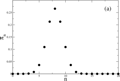
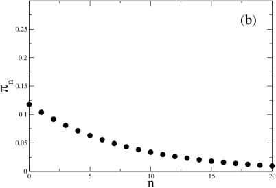
Figure 4: Two possible shapes for the probability distribution $\pi_{n}$ of the number $n$ of particles in a box $B$ of volume $l^{d}$. (a) For a quasi-condensate with an appropriate choice of $l$: the most probable value is $>0$, $\pi_{n}$ is approximately Gaussian with a standard deviation smaller than the mean value. (b) For an ideal Bose gas in the absence of Bose condensate: the most probable value is $n=0$, $\pi_{n}$ is essential an exponential function of $n$. The mean value of $n$ is 8 in both examples.

2.1.3 A solution to these three problems

The introduction of a finite size box is a key ingredient of the previous subsection 2.1.2. We therefore discretize the real space on a grid with a step $l$, a square grid in 2D and a cubic grid in 3D. The position $\mathbf{r}$ now refers to the coordinates of the center of each cell. The field operator $\hat{\psi}(\mathbf{r})$ annihilates a particle in the cell of center $\mathbf{r}$ and is normalized in such a way that

$$[\hat{\psi}(\mathbf{r}),\hat{\psi}^{\dagger}(\mathbf{r}^{\prime})]=\frac{\delta_{\mathbf{r},\mathbf{r}^{\prime}}}{l^{d}}$$ (116)

to recover the usual continuous quantum field theory for $l\rightarrow 0$. We use periodic boundary conditions with lengths that are integer multiple of $l$.

Solution to problem 1: the interaction potential is modeled by a discrete delta potential

$$V(\mathbf{r}-\mathbf{r}^{\prime})=\frac{g_{0}}{l^{d}}\delta_{\mathbf{r},\mathbf{r}^{\prime}}$$ (117)

where the choice of the so-called bare coupling constant $g_{0}$ is discussed later. Note that, in 2D and 3D, $g_{0}$ strongly depends on $l$ in the limit $l\rightarrow 0$, which is a signature of the pathology of a Dirac delta potential in a continuous 2D or 3D space.

The grand canonical model Hamiltonian in second quantized form is then

$$\hat{H}=\sum_{\mathbf{r}}l^{d}\left[-\frac{\hbar^{2}}{2m}\hat{\psi}^{\dagger}(\mathbf{r})\Delta\hat{\psi}(\mathbf{r})+(U(\mathbf{r})-\mu)\hat{\psi}^{\dagger}(\mathbf{r})\hat{\psi}(\mathbf{r})+\frac{g_{0}}{2}\hat{\psi}^{\dagger 2}(\mathbf{r})\hat{\psi}^{2}(\mathbf{r})\right]$$ (118)

where we have introduced the discrete Laplacian $\Delta$. In the initial stage of the Bogoliubov approach to come, it is convenient to represent this discrete Laplacian by

$$\Delta f(\mathbf{r})=\sum_{j\in d\ {\rm directions\ of\ space}}\frac{f(\mathbf{r}+l\mathbf{e}_{j})+f(\mathbf{r}-l\mathbf{e}_{j})-2f(\mathbf{r})}{l^{2}}.$$ (119)

In this case our Hamiltonian becomes fully equivalent to the Bose Hubbard model with an on-site interaction $U=g_{0}/l^{d}$ and a tunneling amplitude $t=-\hbar^{2}/2ml^{2}$. The price to pay is that the dispersion relation of the kinetic energy term is

$$\epsilon_{\mathbf{k}}^{\mathrm{kin}}=\frac{\hbar^{2}}{ml^{2}}\sum_{j=1}^{d}\left(1-\cos k_{j}l\right)$$ (120)

which coincides with the correct parabola only in the range $kl\ll 1$. In the final use of the results derived by the Bogoliubov approach, in particular in a numerical treatment for the spatially inhomogeneous case, it is therefore more accurate to define $\Delta$ in Fourier space, simply by the requirement that the plane wave of wavector $\mathbf{k}$ is an eigenstate with eigenvalue $\hbar^{2}k^{2}/2m$, each component $k_{j}$ of the wavevector being restricted to the first Brillouin zone $[-\pi/l,\pi/l[$.

Solution to problem 2: the variance of the density is finite. In the discrete model, the operator giving the density is $\hat{\rho}(\mathbf{r})=\hat{\psi}^{\dagger}(\mathbf{r})\hat{\psi}(\mathbf{r})$ and has the physical meaning of being equal to $l^{-d}\hat{n}$ where $\hat{n}$ is the operator giving the number of particles in the considered cell. The same phenomenon as in §2.1.2 takes place, the variance of $\hat{\rho}$ is finite:

$$\mbox{Var}\,\hat{\rho}=\frac{\rho}{l^{d}}+[\langle\hat{\psi}^{\dagger 2}\hat{\psi}^{2}\rangle-\rho^{2}]$$ (121)

where $\rho$ is the mean density in the considered cell. We assume that both terms in the right hand side of (121) are much smaller than $\rho^{2}$:

$$\rho l^{d} \gg 1$$ (122)

$$|\langle\hat{\psi}^{\dagger 2}\hat{\psi}^{2}\rangle-\rho^{2}|\ll\rho^{2}.$$ (123)

The first condition ensures that the cell has a large occupation, and the second one ensures that the density fluctuations are weak.

Solution to problem 3: approximate construction of the phase operator. Following [23, 24] one can introduce the exact writing

$$\hat{\psi}\equiv\hat{A}\sqrt{\hat{\rho}}$$ (124)

where $\hat{A}$ decreases the number of particles in the cell by one with an amplitude one rather than $\sqrt{n}$:

$$\hat{A}|n\rangle = |n-1\rangle\ \ \ \mbox{if}\ \ n>0$$ (125)

$$= 0\ \ \ \mbox{otherwise}.$$ (126)

The following identities are exact:

$$\hat{A}\hat{A}^{\dagger} = 1$$ (127)

$$\hat{A}^{\dagger}\hat{A} = 1-|0\rangle\langle 0|$$ (128)

where $|0\rangle$ is the vacuum state of the considered cell. This reveals that $\hat{A}$ is not unitary. However if the probability of having no particle in the cell is truly negligible in the state on which $\hat{A}$ acts, the overlap of this state with $|0\rangle\langle 0|$ can be neglected and one can assume that $\hat{A}$ is unitary:

$$\hat{A}^{\dagger}\hat{A}\simeq\hat{A}\hat{A}^{\dagger}=1.$$ (129)

One then can set

$$\hat{A}=e^{i\hat{\theta}}$$ (130)

where $\hat{\theta}$ is Hermitian. The commutation relation (101) is then an acceptable approximation that ensures e.g. that

$$\hat{A}^{\dagger}\hat{\rho}\hat{A}\simeq\hat{\rho}-\frac{1}{l^{d}}.$$ (131)

We note that there exists rigorous definitions of the phase operator [25], but the resulting operator does not satisfy (101), which makes explicit calculations more difficult.

2.1.4 How to choose the grid spacing $l$ ?

A first condition is that $l$ is large enough so that $\rho l^{d}\gg 1$. Note that the model Hamiltonian (118) can be used outside this regime, this condition being useful only for the Bogoliubov approximation to come.

A second condition is that $l$ is small enough so that the energy cut-off $\sim\hbar^{2}/ml^{2}$ introduced by the grid does not change the physics. This obviously requires that the energy cut-off is larger than $k_{B}T$ and than the chemical potential $\mu$. Equivalently

$$l<\lambda,\xi$$ (132)

where $\lambda$ is the thermal de Broglie wavelength and $\xi$ is the healing length defined in (98).

These three conditions are compatible only in the degenerate (96) and weakly interacting (97) regime to which our Bogoliubov approach is therefore restricted.

2.1.5 How to choose the coupling constant $g_{0}$ ?

The idea is the following. Consider the scattering of a plane wave on the discrete $\delta$ potential on the grid, for a finite grid spacing $l$ but of course in the case of an infinite quantization volume. Calculate the corresponding scattering amplitude and compare it to the exact amplitude for the true interaction potential in continuous space. Adjust $g_{0}$ to have the same scattering amplitude in the low energy domain.

Let us calculate the $T$ matrix for two interacting particles in the discrete model. We take the version of the discrete Laplacian giving the correct parabolic spectrum, as discussed after (120). The center of mass motion can be separated from the relative motion so we consider the reduced Hamiltonian for the relative motion of the two particles on the grid:

$$H=\frac{p^{2}}{m}+V$$ (133)

with $V=g_{0}\delta_{\mathbf{r},\mathbf{0}}/l^{d}$. The eigenstates of the kinetic energy are plane waves with a wavevector $\mathbf{k}$, with a wavefunction

$$\langle\mathbf{r}|\mathbf{k}\rangle=e^{i\mathbf{k}\cdot\mathbf{r}}.$$ (134)

As each component $r_{j}$ is an integer multiple of $l$, the component $k_{j}$ has a meaning modulo $2\pi/l$ and can be restricted to the first Brillouin zone $[-\pi/l,\pi/l[$. We normalize the localized state vector $|\mathbf{r}\rangle$ so as to recover the continuous theory for $l\rightarrow 0$:

$$\langle\mathbf{r}|\mathbf{r}^{\prime}\rangle=\frac{\delta_{\mathbf{r},\mathbf{r}^{\prime}}}{l^{d}}.$$ (135)

In this case the potential $V$ can be written as

$$V=g_{0}|\mathbf{r}=\mathbf{0}\rangle\langle\mathbf{r}=\mathbf{0}|$$ (136)

and the following closure relation holds:

$$\int_{D}\frac{d^{d}\mathbf{k}}{(2\pi)^{d}}|\mathbf{k}\rangle\langle\mathbf{k}|=1$$ (137)

where $D=[-\pi/l,\pi/l[^{d}$ is the first Brillouin zone of the reciprocal lattice.

The $T$ matrix at a given energy $E$ is defined by [26]:

$$T(E+i\eta)=V+VG(E+i\eta)V$$ (138)

where $\eta\rightarrow 0^{+}$ at the end of the calculation. $G$ is the resolvent of the full Hamiltonian:

$$G(z)=\frac{1}{z-H}$$ (139)

defined for any complex number $z$ not belonging to the spectrum of $H$. The particular form of $V$ leads to the simple expression for the matrix element of $T$ in between two arbitrary plane waves [27]:

$$\langle\mathbf{k}|T_{\rm grid}(E+i\eta)|\mathbf{k}^{\prime}\rangle=g_{0}+g_{0}^{2}\langle\mathbf{r}=\mathbf{0}|G(E+i\eta)|\mathbf{r}=\mathbf{0}\rangle$$ (140)

so that only the matrix element of the resolvent in the state localized in the cell $\mathbf{r}=\mathbf{0}$ of the lattice matters! This matrix element is immediately deduced from the recursion relation

$$G(z)=G_{0}(z)+G_{0}(z)VG(z)$$ (141)

where $G_{0}$ is the resolvent of the kinetic energy operator. We finally obtain

$$\langle\mathbf{k}|T_{\rm grid}(E+i\eta)|\mathbf{k}^{\prime}\rangle=\frac{g_{0}}{1-g_{0}I(E)}$$ (142)

where

$$I(E)=\langle\mathbf{r}=\mathbf{0}|G_{0}(E+i\eta)|\mathbf{r}=\mathbf{0}\rangle=\lim_{\eta\rightarrow 0^{+}}\int_{D}\frac{d^{d}\mathbf{k}}{(2\pi)^{d}}\frac{1}{E+i\eta-\hbar^{2}k^{2}/m}.$$ (143)

Note that, due to the discrete delta nature of the interaction potential, the matrix element of $T_{\rm grid}$ depends only on the energy, not on the wavevectors: the operator $T_{\rm grid}$ is actually proportional to $|\mathbf{r}=\mathbf{0}\rangle\langle\mathbf{r}=\mathbf{0}|$.

To calculate $I(E)$ one may use the following identity for distributions:

$$\lim_{\eta\rightarrow 0^{+}}\frac{1}{X+i\eta}={\cal PP}\frac{1}{X}-i\pi\delta(X)$$ (144)

where ${\cal PP}$ is the principal part. We restrict to positive energies $E$ and we set $E=\hbar^{2}q^{2}/m$. We are interested in the low energy limit $E\ll\hbar^{2}/ml^{2}$ that is $q\ll\pi/l$. Why ? In the degenerate and weakly interacting regime the maximal value of $q$ is $1/\xi$ or $1/\lambda$, which is much smaller than $1/l$.

The imaginary part of $I(E)$ is easy to calculate when $q<\pi/l$, in which case the support of the $\delta$ distribution is inside the Brillouin zone $D$ and $\mbox{Im}\,I(E)$ is proportional to the density of states:

$$\begin{array}[]{ccccc}\mbox{Im}\,I(E)&=&\displaystyle-\frac{m}{4\pi\hbar^{2}}q&\mbox{in 3D}&\\ &&&&\\ &=&\displaystyle-\frac{m}{4\hbar^{2}}&\mbox{in 2D}&\ \ \ \ \mathrm{for}\ \ q<\pi/l\\ &&&&\\ &=&\displaystyle-\frac{m}{2\hbar^{2}}\frac{1}{q}&\mbox{in 1D}&\end{array}$$ (145)

The calculation of the real part of $I(E)$ is more involved:

$$\mbox{Re}\,I(E)=\frac{m}{\hbar^{2}}\int_{D}\frac{d^{d}\mathbf{k}}{(2\pi)^{d}}{\cal PP}\frac{1}{q^{2}-k^{2}}$$ (146)

so we shall restrict to the low energy limit. In 3D, the real part has a finite limit for $q\rightarrow 0$: replacing $q$ by zero, one obtains

$$\mbox{Re}\,I(E=0) = \frac{m}{\hbar^{2}}\int_{D}\frac{d^{3}\mathbf{k}}{(2\pi)^{3}}\frac{1}{k^{2}}$$ (147)

$$= \frac{m}{\hbar^{2}l}\times 0.194\ldots$$ (148)

The situation is dramatically different in 2D, where one gets a divergent expression if one replaces $q$ by zero. The trick is then to split the integration domain $D$ in the disk of radius $\pi/l$, over which the integral can be calculated exactly, and in the complementary domain, where $q^{2}$ is a small perturbation of $k^{2}$ [28]:

$$\mbox{Re}\,I(E)=\frac{m}{2\pi\hbar^{2}}\left[\ln(ql/\pi)-C+O((ql)^{2})\right]$$ (149)

with the constant

$$C=\ln 2-\frac{2}{\pi}G=0.110025\ldots$$ (150)

involving Catalan’s constant $G=0.915965594\ldots$. In 1D the exact calculation can be done:

$$\mbox{Re}\,I(E)=\frac{m}{2\pi\hbar^{2}q}\ln\left|\frac{\pi+ql}{\pi-ql}\right|\sim_{ql\rightarrow 0}\frac{ml}{\pi^{2}\hbar^{2}}.$$ (151)

The last step is to compare with the scattering amplitude of the true interaction potential in the continuous case. In 3D a low energy approximation can be used for the true $T$ matrix:

$$\langle\mathbf{k}|T_{\rm true}(E+i\eta)|\mathbf{k}^{\prime}\rangle\simeq\frac{4\pi\hbar^{2}/m}{\frac{1}{a}+iq},$$ (152)

where $a$ is the $s$-wave scattering length, provided that $kr_{e},k^{\prime}r_{e},qr_{e}\ll 1$, where $r_{e}$ is the effective range of the true interaction potential. The maximal value of $q,k,k^{\prime}$ that one may expect to appear in the thermal state of the gas in the degenerate regime is the inverse of the mean interparticle separation $\rho^{1/3}$, whatever the strength of the interactions: one has to check that $\rho r_{e}^{3}\ll 1$, which is the case in present experiments even close to a Feshbach resonance [29]. In the weakly interacting regime, the situation is even more favorable as the typical $q,k,k^{\prime}$ is at most $1/\xi$ or $1/\lambda$, much smaller than $\rho^{1/3}$.

Using the expressions (148) and (145) for $I(E)$ and identifying $T_{\rm grid}$ with $T_{\rm true}$ leads to the identity

$$\frac{1}{g_{0}}=\frac{m}{4\pi\hbar^{2}a}-\frac{m}{\hbar^{2}}\int_{D}\frac{d^{3}\mathbf{k}}{(2\pi)^{3}}\frac{1}{k^{2}}$$ (153)

that is

$$g_{0}=\frac{4\pi\hbar^{2}a/m}{1-K_{3}a/l}\ \ \ \mbox{with}\ \ K_{3}=2.442\,749\ldots$$ (154)

Note the exact cancellation of the imaginary parts of the denominators of $T_{\rm grid}$ and $T_{\rm true}$. In the considered weakly interacting regime, condition (97) implies $\sqrt{\rho a^{3}}\ll 1$; as $\rho l^{3}\gg 1$ one finds that $a\ll l$ so that $g_{0}$ is close to the usual coupling constant $g=4\pi\hbar^{2}a/m$. Close, but not identical, and this plays an important role in suppressing potential ultraviolet divergences.

In 2D, the low energy approximation for the ‘true’ $T$ matrix is

$$\langle\mathbf{k}|T_{\rm true}(E+i\eta)|\mathbf{k}^{\prime}\rangle\simeq\frac{-2\pi\hbar^{2}/m}{\ln(a_{2}q/2)+\gamma-i\pi/2}$$ (155)

where $a_{2}$ is the 2D scattering length and $\gamma=0.57721\ldots$ is Euler’s constant, see the lecture of Gora Shlyapnikov in this volume. In identifying with the low energy expression of $T_{\rm grid}$, one finds again that the imaginary parts of the denominators of $T_{\rm grid}$ and $T_{\rm true}$ exactly cancel and one is left with:

$$g_{0}=\frac{2\pi\hbar^{2}}{m}\frac{1}{\ln(K_{2}l/a_{2})}$$ (156)

with a numerical constant

$$K_{2}=\frac{1}{\pi}e^{-\gamma+2G/\pi}\simeq\frac{1}{\pi}$$ (157)

where we used the amusing fact that $-\gamma+2G/\pi=5.91\ldots 10^{-3}\ll 1$.

In 1D one may model the continuous interaction potential by $g_{1}\delta(z_{1}-z_{2})$, under validity conditions discussed in [30, 31], in which case the $T$ matrix is

$$\langle k|T_{\rm true}(E+i\eta)|k^{\prime}\rangle\simeq\frac{\hbar^{2}/m}{a_{1}+i/2q}$$ (158)

where the 1D scattering length is such that

$$g_{1}=\frac{\hbar^{2}}{ma_{1}}.$$ (159)

The identification of $T_{\rm grid}$ and $T_{\rm true}$ leads to

$$g_{0}=\frac{g_{1}}{1+l/(a_{1}\pi^{2})}.$$ (160)

In the weakly interacting regime, $g_{0}$ is very close to $g_{1}$: $l\ll\xi$, so that $l/a_{1}\ll\xi/a_{1}\propto 1/\sqrt{\rho a_{1}}\propto 1/\rho\xi\ll 1$. Contrarily to the 3D case, the small difference between $g_{0}$ and $g_{1}$ does not play a significant role.

2.2 Perturbative expansion of the model Hamiltonian

In a regime where each cell has a negligible probability of being empty, we may introduce the phase operator having approximately the commutation relation (101) with the density and write the Hamiltonian as

$$\hat{H} = \hat{H}_{\rm kin}+\hat{H}_{\rm pot}$$ (161)

$$\hat{H}_{\rm pot} = \sum_{\mathbf{r}}l^{d}\hat{\rho}(\mathbf{r})\left[U(\mathbf{r})-\mu+\frac{g_{0}}{2}\left(\hat{\rho}(\mathbf{r})-\frac{1}{l^{d}}\right)\right]$$ (162)

$$\hat{H}_{\rm kin} \simeq -\frac{\hbar^{2}}{2ml^{2}}\sum_{\mathbf{r}}l^{d}\sum_{j=1}^{d}\left\{\left[\hat{\rho}^{1/2}e^{i(\hat{\theta}_{+j}-\hat{\theta})}\hat{\rho}_{+j}^{1/2}+\mbox{h.c.}\right]-2\hat{\rho}\right\}$$ (163)

where we have introduced the notation

$$f_{+j} = f(\mathbf{r}+l\mathbf{e}_{j})$$ (164)

$$f_{-j} = f(\mathbf{r}-l\mathbf{e}_{j})$$ (165)

for each direction of space.

2.2.1 Two small parameters

The first small parameter expresses the weakness of the density fluctuations: one splits

$$\hat{\rho}(\mathbf{r})=\rho_{0}(\mathbf{r})+\delta\hat{\rho}(\mathbf{r})$$ (166)

where $\rho_{0}$, the zeroth order approximation to the density, corresponds to a pure quasi-condensate. The small parameter is then

$$\epsilon_{1}=\frac{|\delta\hat{\rho}|}{\rho_{0}}\ll 1.$$ (167)

The second small parameter expresses the smallness of the phase variation in between neighboring sites of the grid:

$$\epsilon_{2}=|l\,\mathbf{grad}\,\hat{\theta}|\ll 1$$ (168)

where $\mathbf{grad}$ is the discrete gradient on the lattice.

It can be checked at the end of all calculations that by an appropriate choice of $l$ one can achieve

$$\epsilon_{1}\sim\epsilon_{2}\sim\frac{1}{\sqrt{\rho_{0}l^{d}}}.$$ (169)

One may note that this value corresponds to the ‘quantum’ fluctuation part, that is the first term in the right-hand side of (121). An important consequence is that the two small parameters may be considered as a single small parameter, in the expansion of the Hamiltonian.

2.2.2 Quadratisation of the Hamiltonian

Expansion of $\hat{H}$ in powers of $\epsilon_{1}$ and $\epsilon_{2}$ is performed from the series expansions

$$\hat{\rho}^{1/2} = \rho_{0}^{1/2}+\frac{\delta\hat{\rho}}{2\rho_{0}^{1/2}}-\frac{\delta\hat{\rho}^{2}}{8\rho_{0}^{3/2}}+\frac{\delta\hat{\rho}^{3}}{16\rho_{0}^{5/2}}+\ldots$$ (170)

$$e^{i(\hat{\theta}_{+j}-\hat{\theta})} = 1+i(\hat{\theta}_{+j}-\hat{\theta})-\frac{1}{2}(\hat{\theta}_{+j}-\hat{\theta})^{2}+\ldots$$ (171)

To zeroth order in the small parameters $\epsilon_{1}$ and $\epsilon_{2}$, density fluctuations are neglected, $\hat{\rho}$ being approximated by $\rho_{0}$, and the spatial variation of the phase operator is also neglected. This leads to the zeroth order approximation to the Hamiltonian, which is the following c-number:

$$H_{0}=\sum_{\mathbf{r}}l^{d}\rho_{0}^{1/2}\left[-\frac{\hbar^{2}}{2m}\Delta+U(\mathbf{r})+\frac{1}{2}g_{0}\rho_{0}-\mu\right]\rho_{0}^{1/2}.$$ (172)

In 3D, this is the equivalent on the lattice of the Gross-Pitaevskii energy functional, with the difference that the bare coupling constant $g_{0}$ appears, rather than $g$. $\rho_{0}$ is then naturally obtained by minimization of $H_{0}$, so that it obeys:

$$\left[-\frac{\hbar^{2}}{2m}\Delta+U(\mathbf{r})+g_{0}\rho_{0}-\mu\right]\rho_{0}^{1/2}=0.$$ (173)

This equation naturally defines $\rho_{0}$ as a function of $\mu$. However it will reveal more convenient to parameterize the theory in terms of $N_{0}$, i.e. the total number of particles stored in the density profile $\rho_{0}$:

$$N_{0}=\sum_{\mathbf{r}}l^{d}\rho_{0}(\mathbf{r}).$$ (174)

We will therefore consider $\mu$ and $\rho_{0}$ as functions of $N_{0}$:

$$\mu = \mu_{0}(N_{0})$$ (175)

$$\rho_{0}(\mathbf{r}) = \rho_{0}(\mathbf{r};N_{0}).$$ (176)

As a consequence of Eq.(173), one finds that the first order approximation $\hat{H}_{1}$ to the Hamiltonian exactly vanishes. The first non-trivial contribution is therefore a quadratic one:

$$\hat{H}_{2} = E_{2}[\rho_{0}]+\sum_{\mathbf{r}}l^{d}\left[-\frac{\hbar^{2}}{2m}\frac{\delta\hat{\rho}}{2\sqrt{\rho_{0}}}\Delta\left(\frac{\delta\hat{\rho}}{2\sqrt{\rho_{0}}}\right)+\frac{\hbar^{2}\delta\hat{\rho}^{2}}{8m\rho_{0}^{3/2}}\Delta\sqrt{\rho_{0}}+\frac{g_{0}}{2}\delta\hat{\rho}^{2}\right.$$ (177)

$$+ \left.\frac{\hbar^{2}}{2m}\sum_{j}\sqrt{\rho_{0}(\mathbf{r})\rho_{0}(\mathbf{r}+l{\bf e_{j}})}\,\frac{(\hat{\theta}(\mathbf{r}+l{\bf e_{j}})-\hat{\theta}(\mathbf{r}))^{2}}{l^{2}}\right]$$ (178)

where the c-number energy functional $E_{2}[\rho_{0}]$ is given by

$$E_{2}[\rho_{0}]=-\frac{g_{0}}{2}\sum_{\mathbf{r}}\rho_{0}-\frac{\hbar^{2}}{4ml^{2}}\sum_{\mathbf{r}}\sum_{j=1}^{d}\left[\left(\frac{\rho_{0,+j}}{\rho_{0}}\right)^{1/2}+\left(\frac{\rho_{0}}{\rho_{0,+j}}\right)^{1/2}\right].$$ (180)

Remarkably, one finds that the Hamiltonian $\hat{H}_{2}$ is equivalent to the Hamiltonian of the $U(1)$-symmetry breaking Bogoliubov approach for the usual case of true condensates: one introduces the field

$$\hat{B}(\mathbf{r})=\frac{\delta\hat{\rho}(\mathbf{r})}{2\rho_{0}^{1/2}(\mathbf{r})}+i\rho_{0}^{1/2}(\mathbf{r})\hat{\theta}(\mathbf{r}).$$ (181)

One can then check that it has bosonic commutation relations

$$[\hat{B}(\mathbf{r}),\hat{B}^{\dagger}(\mathbf{r}^{\prime})]=\frac{\delta_{\mathbf{r},\mathbf{r}^{\prime}}}{l^{d}}.$$ (182)

After some algebra, using the fact that $\rho_{0}^{1/2}$ solves the Gross-Pitaevskii type equation (173), one obtains the following exact rewriting of $\hat{H}_{2}$:

$$\hat{H}_{2}=l^{d}\sum_{\mathbf{r}}\hat{B}^{\dagger}\left(-\frac{\hbar^{2}}{2m}\Delta+U+g_{0}\rho_{0}-\mu\right)\hat{B}+g_{0}\rho_{0}\left[\hat{B}^{\dagger}\hat{B}+\frac{1}{2}(\hat{B}^{2}+\hat{B}^{\dagger 2})\right]$$ (183)

which has exactly the structure of the usual Bogoliubov Hamiltonian. Remarkably, the c-number energy $E_{2}$ is exactly compensated by the contribution of commutators of $\delta\hat{\rho}$ with $\hat{\theta}$. One then reuses the standard diagonalization of the Bogoliubov Hamiltonian:

$$\hat{B}(\mathbf{r})=-i\hat{Q}\rho_{0}^{1/2}(\mathbf{r})+\hat{P}\partial_{N_{0}}\rho_{0}^{1/2}(\mathbf{r})+\sum_{s}\hat{b}_{s}u_{s}(\mathbf{r})+\hat{b}^{\dagger}_{s}v_{s}^{*}(\mathbf{r})$$ (184)

as explained in [32, 33, 24]. Here the sum $s$ is taken over the regular Bogoliubov eigenmodes $(u_{s},v_{s})$

$$\left(\begin{array}[]{cc}-\frac{\hbar^{2}}{2m}\Delta+U-\mu+2g_{0}\rho_{0}&g_{0}\rho_{0}\\ -g_{0}\rho_{0}&-\left(-\frac{\hbar^{2}}{2m}\Delta+U-\mu+2g_{0}\rho_{0}\right)\end{array}\right)\left(\begin{array}[]{c}u_{s}\\ v_{s}\end{array}\right)=\epsilon_{s}\left(\begin{array}[]{c}u_{s}\\ v_{s}\end{array}\right)$$ (185)

normalizable as

$$\sum_{\mathbf{r}}l^{d}\left[|u_{s}(\mathbf{r})|^{2}-|v_{s}(\mathbf{r})|^{2}\right]=1.$$ (186)

Thermodynamic stability, or equivalently the fact that $\rho_{0}$ is a minimum of $H_{0}$, imposes that the corresponding eigenenergies $\epsilon_{s}$ are positive [1]. The operators $\hat{b}_{s}$ obey the usual bosonic commutation relations $[\hat{b}_{s},\hat{b}^{\dagger}_{s^{\prime}}]=\delta_{s,s^{\prime}}$. The operators $\hat{Q}$ and $\hat{P}$ commute with $\hat{b}_{s},\hat{b}_{s}^{\dagger}$ and are conjugate quantum variables,

$$[\hat{P},\hat{Q}]=-i.$$ (187)

$\hat{Q}$ is a collective coordinate representing the quantum phase of the field, and, as shown in [28], $\hat{P}$ gives the fluctuations of the total number of particles away from the total number of particles $N_{0}$ contained in the density profile $\rho_{0}$:

$$\hat{P}=l^{d}\sum_{\mathbf{r}}[\hat{\rho}(\mathbf{r})-\rho_{0}(\mathbf{r})]=\hat{N}-N_{0}.$$ (188)

We note that our treatment is in the grand canonical ensemble but does not break the $U(1)$-symmetry of the Hamiltonian: the emergence of the operators $\hat{P}$ and $\hat{Q}$ is therefore a consequence of a non-fixed value of the total number of particles, rather than of symmetry breaking.

Replacing $\hat{B}$ by the Bogoliubov modal decomposition finally leads to a modal expansion for the operators giving the density and the phase:

$$\hat{\theta}(\mathbf{r}) = -\hat{Q}+\sum_{s}\theta_{s}(\mathbf{r})\,\hat{b}_{s}+\theta_{s}^{*}(\mathbf{r})\hat{b}_{s}^{\dagger}$$ (189)

$$\delta\hat{\rho}(\mathbf{r}) = \hat{P}\partial_{N_{0}}\rho_{0}(\mathbf{r})+\sum_{s}\delta\rho_{s}(\mathbf{r})\hat{b}_{s}+\delta\rho_{s}^{*}(\mathbf{r})\hat{b}_{s}^{\dagger}$$ (190)

where

$$\theta_{s}(\mathbf{r}) = \frac{u_{s}(\mathbf{r})-v_{s}(\mathbf{r})}{2i\rho_{0}^{1/2}(\mathbf{r})}$$ (191)

$$\delta\rho_{s}(\mathbf{r}) = \rho_{0}^{1/2}(\mathbf{r})[u_{s}(\mathbf{r})+v_{s}(\mathbf{r})].$$ (192)

It also gives the normal form of the Hamiltonian $\hat{H}_{2}$, from which thermal averages can be evaluated easily:

$$\hat{H}_{2}=-\frac{1}{2}N_{0}\frac{d\mu_{0}}{dN_{0}}-\sum_{s}\epsilon_{s}\langle v_{s}|v_{s}\rangle+\frac{1}{2}\frac{d\mu_{0}}{dN_{0}}\hat{P}^{2}+\sum_{s}\epsilon_{s}\hat{b}_{s}^{\dagger}\hat{b}_{s}$$ (193)

where the function $\mu_{0}$ is defined in Eq.(175) [34].

2.2.3 Why cubic terms in the Hamiltonian are required

One could believe that the knowledge of $\hat{H}_{2}$ is sufficiently to calculate to a given order $O(\epsilon_{1,2}^{2})$ the correction for any observable to the pure quasi-condensate approximation. However this is not true, the mean density being an obvious counter-example: in a thermal state density operator with the Hamiltonian $\hat{H}_{2}$, the mean value of $\delta\hat{\rho}$ vanishes so that, for a given chemical potential, there is no correction to the mean density as compared to the pure quasi-condensate assumption.

A similar phenomenon takes place in the quantum mechanical problem of a single particle strongly confined in a non-harmonic trapping potential $V(x)$ in 1D: a series expansion of the potential is performed around its minimum,

$$V(x)=V_{0}+\frac{1}{2}V^{\prime\prime}(x_{0})(x-x_{0})^{2}+\frac{1}{6}V^{(3)}(x-x_{0})^{3}+\ldots$$ (194)

where $x$ is the particle coordinate. To zeroth order in the expansion, the ground state energy of the particle is $V_{0}$ and its position is $x_{0}$. The first correction to the energy is given by the inclusion of the quadratic term of Eq.(194) and, when expressed in units of $V_{0}$, it scales as $V^{\prime\prime 1/2}/V_{0}\sim 1/(V_{0}^{1/2}x_{0})$ where $x_{0}$ is assumed to be also a typical length scale of $V(x)$. The first correction to the mean position of the particle is given by the inclusion of the cubic term in Eq.(194) as a perturbation to the harmonic potential and, when expressed in units of $x_{0}$, scales also as $1/(V_{0}^{1/2}x_{0})$!

Coming back to the quantum gas problem, one has to produce a third order expansion of the model Hamiltonian and treat the resulting cubic Hamiltonian $\hat{H}_{3}$ as a perturbation to $\hat{H}_{2}$. The derivation of $\hat{H}_{3}$ is detailed in an appendix of [28], we give here only the result:

$$\hat{H}_{3} = -\frac{g_{0}}{2}\sum_{\mathbf{r}}\delta\hat{\rho}+\frac{\hbar^{2}}{4ml^{2}}\sum_{\mathbf{r},j}l^{d}\,(\hat{\theta}_{+j}-\hat{\theta})\left(\frac{\rho_{0,+j}^{1/2}}{\rho_{0}^{1/2}}\,\delta\hat{\rho}+\frac{\rho_{0}^{1/2}}{\rho_{0,+j}^{1/2}}\,\delta\hat{\rho}_{+j}\right)(\hat{\theta}_{+j}-\hat{\theta})$$

$$+ \frac{\hbar^{2}}{8m}\sum_{\mathbf{r}}\frac{\delta\hat{\rho}}{\rho_{0}}\left(\rho_{0}^{-1/2}\Delta\rho_{0}^{1/2}-\rho_{0}^{1/2}\Delta\rho_{0}^{-1/2}\right)-\frac{\hbar^{2}}{16m}\sum_{\mathbf{r}}l^{D}\left[\frac{\delta\hat{\rho}^{3}}{\rho_{0}^{5/2}}\Delta\sqrt{\rho_{0}}-\frac{\delta\hat{\rho}^{2}}{\rho_{0}^{3/2}}\Delta\left(\frac{\delta\hat{\rho}}{\sqrt{\rho_{0}}}\right)\right].$$

There are then two main ways to calculate the correction to the mean density due to $\hat{H}_{3}$. The first one relies on finite temperature perturbation theory: to calculate expectation values in the density operator $\exp[-\beta(\hat{H}_{2}+\hat{H}_{3})]$ to first order in $\hat{H}_{3}$, one uses the imaginary time version of the time dependent first order perturbation theory:

$$e^{-\beta(\hat{H}_{2}+\hat{H}_{3})}=e^{-\beta\hat{H}_{2}}-\int_{0}^{\beta}d\tau\,e^{-(\beta-\tau)\hat{H}_{2}}\hat{H}_{3}e^{-\tau\hat{H}_{2}}+\ldots$$ (196)

One is then back to the calculation of expectation values of operators in the thermal state corresponding to $\hat{H}_{2}$, and Wick’s theorem can be applied.

The second way to include the effect of $\hat{H}_{3}$ perturbatively is here simpler and was followed in [28]. It consists in writing the equation of motion of $\hat{\theta}$ in Heisenberg representation for the Hamiltonian $\hat{H}_{2}+\hat{H}_{3}$: with respect to the evolution governed by $\hat{H}_{2}$, ‘new’ terms appear. One then takes the expectation value of this equation in the desired thermal state. The expectation value of the ‘new’ terms can be taken in the unperturbed thermal state, as they originate from the perturbation $\hat{H}_{3}$. Furthermore the expectation value of $\partial_{t}\hat{\theta}$ vanishes in steady state, as proved in an appendix of [28], so that

$$0 = \left[-\frac{\hbar^{2}}{2m}\Delta+U+3g_{0}\rho_{0}-\mu\right]\left(\frac{\langle\delta\hat{\rho}\rangle_{3}-\langle\hat{B}^{\dagger}\hat{B}\rangle_{2}}{\rho_{0}^{1/2}}\right)$$ (197)

$$+ g_{0}\rho_{0}^{1/2}\langle 4\hat{B}^{\dagger}\hat{B}+\hat{B}^{2}+\hat{B}^{\dagger 2}\rangle_{2}-2\langle\hat{P}^{2}\rangle_{2}\frac{d\mu_{0}}{dN_{0}}\partial_{N_{0}}\sqrt{\rho_{0}}$$

where the thermal average $\langle\ldots\rangle_{2}$ is taken with the unperturbed Hamiltonian $\hat{H}_{2}$ and $\langle\ldots\rangle_{3}$ is taken with the perturbed Hamiltonian $\hat{H}_{2}+\hat{H}_{3}$ to first order in $\hat{H}_{3}$. The fact that $\rho_{0}$ is a minimum of $H_{0}$ imposes that the differential operator in the first line of Eq.(197) is strictly positive [24, 1] so that this equation determines $\langle\delta\hat{\rho}\rangle_{3}$ in a unique way.

2.3 Applications of the formalism

We present here without derivation simple applications of the expansion of the Hamiltonian performed in the previous subsection. For simplicity, we restrict to the spatially homogeneous case of a gas with periodic boundary conditions in a box of size $L$ along each direction of space and we take the thermodynamic limit $L\rightarrow+\infty$ for a fixed value of the chemical potential. The derivation of the formulas given below and their extension to the case of a finite size, spatially inhomogeneous system can be found in [28].

2.3.1 Equation of state

Thanks to Eq.(197) we can relate the mean density to the chemical potential to first order beyond the pure quasi-condensate approximation. As derived in [28]

$$\frac{\mu}{g_{0}}=\rho+\int_{D}\frac{d^{d}\mathbf{k}}{(2\pi)^{d}}\left[(U_{k}+V_{k})^{2}n_{k}+V_{k}(U_{k}+V_{k})\right]$$ (198)

where $n_{k}=1/[\exp(\beta\epsilon_{k})-1]$ is the mean occupation number of the Bogoliubov mode of wavevector $\mathbf{k}$ and $U_{k},V_{k}$ are the amplitudes of the Bogoliubov mode functions $u_{\mathbf{k}}(\mathbf{r})=U_{k}\exp(i\mathbf{k}\cdot\mathbf{r})/L^{d/2}$ and $v_{\mathbf{k}}(\mathbf{r})=V_{k}\exp(i\mathbf{k}\cdot\mathbf{r})/L^{d/2}$:

$$U_{k}+V_{k}=\frac{1}{U_{k}-V_{k}}=\left[\frac{\hbar^{2}k^{2}/2m}{2\mu+\hbar^{2}k^{2}/2m}\right]^{1/4}.$$ (199)

The corresponding Bogoliubov eigenenergy is

$$\epsilon_{k}=\left[\frac{\hbar^{2}k^{2}}{2m}\left(\frac{\hbar^{2}k^{2}}{2m}+2\mu\right)\right]^{1/2}.$$ (200)

In what follows we shall need the large $k$ dependence of the zero temperature value of the integrand in Eq.(198):

$$V_{k}(U_{k}+V_{k})\simeq-\frac{m\mu}{\hbar^{2}k^{2}}.$$ (201)

Eq.(198) is not totally satisfactory yet as it depends on the grid spacing $l$ of our lattice model, both through the integration domain $D$ defined after Eq.(137) and through the $l$-dependence of the coupling constant $g_{0}$. Let us check, for each value of the dimension $d$, that the $l$ dependence disappears in the limit $l\ll\xi,\lambda$.

In 1D this is clearly the case as both $g_{0}$ and the integral in Eq.(198) have a finite limit when $l\rightarrow 0$. One can then replace $g_{0}$ by the 1D coupling constant $g_{1}$, and $D$ by $]-\infty,+\infty[$.

In 2D the integral in Eq.(198) diverges logarithmically in the limit $l\rightarrow 0$, because of the $T=0$ contribution to the integrand. We calculate the low-$l$ behavior of the integral by splitting the integration domain $D$ in a disk of radius $\pi/l$, over which the integral is performed in polar coordinates, and a complementary domain, over which the integrand is approximated by its asymptotic behavior Eq.(201). We obtain

$$-\int_{D}\frac{d^{2}\mathbf{k}}{(2\pi)^{2}}\,V_{k}(U_{k}+V_{k})=\frac{m\mu}{4\pi\hbar^{2}}\left[\ln\left(\frac{\pi^{2}\hbar^{2}}{ml^{2}\mu}\right)-1+2\ln 2-4G/\pi+O(l^{2}/\xi^{2})\right]$$ (202)

where $G$ is Catalan’s constant. Remarkably this compensates the logarithmic $l$ dependence in the value of $1/g_{0}$, see Eq.(156). We arrive at the equation of state of the 2D gas:

$$\rho=\frac{m\mu}{4\pi\hbar^{2}}\ln\left(\frac{4\hbar^{2}}{a_{2}^{2}m\mu e^{2\gamma+1}}\right)-\int\frac{d\mathbf{k}}{(2\pi)^{2}}(\bar{u_{k}}+\bar{v_{k}})^{2}n_{k}$$ (203)

where $\gamma$ is Euler’s constant and $a_{2}$ is the 2D scattering length. This relation is identical to the result (20.45) obtained by the functional integral method in [18]. It allows to show that the necessary condition $\rho\xi^{2}\gg 1$ for our treatment to apply imposes $\ln(1/\rho a_{2}^{2})\gg 4\pi$ at zero temperature.

In 3D, the integral in Eq.(198) also diverges. Using the identity Eq.(153) satisfied by the bare coupling constant $g_{0}$ amounts to subtracting the high $k$ behavior of the integrand, so that the $l\rightarrow 0$ limit may be taken to give

$$\mu=\rho g+g\int\frac{d\mathbf{k}}{(2\pi)^{3}}\left((U_{k}+V_{k})^{2}n_{k}+V_{k}(U_{k}+V_{k})+\frac{m\mu}{\hbar^{2}k^{2}}\right).$$ (204)

In 3D our result coincides with the one of the usual Bogoliubov approach for a condensate. What might be surprising at first sight is that our results in 2D and in 1D also coincide with the ones predicted by a blind application of the usual Bogoliubov method, even if there is no true condensate! The same conclusion applies for the ground state energy of a gas of $N$ particles, as shown in [28], and as could be expected from the equivalence of $\hat{H}_{2}$ with the usual Bogoliubov Hamiltonian. This fact that the usual Bogoliubov approach gives the correct result was commonly used in the literature in 1D, see e.g. [5], and was justified by an asymptotic treatment of the solution based on the Bethe ansatz in [7]. With our extended Bogoliubov method, we reach this conclusion in a simpler, more transparent and more general way.

2.3.2 Density fluctuations

Our treatment relies on the assumption of weak density fluctuations. We then have to check that the relative variance of the density fluctuations is weak:

$$\epsilon_{1}^{2}=\frac{\langle\delta\hat{\rho}^{2}(\mathbf{0})\rangle_{2}}{\rho_{0}^{2}}\stackrel{{\scriptstyle?}}{{\ll}}1.$$ (205)

Following the discussion of §2.1.2 we expect this variance to be the sum of two contributions, one coming from the fact that $\delta\hat{\rho}^{2}$ is not a normally ordered operator, and a second one involving the second order correlation function of the field,

$$g_{2}(\mathbf{r})\equiv\langle\hat{\psi}^{\dagger}(\mathbf{r})\hat{\psi}^{\dagger}(\mathbf{0})\hat{\psi}(\mathbf{0})\hat{\psi}(\mathbf{r})\rangle.$$ (206)

Explicit calculations are performed in [28]. In the thermodynamical limit one finds indeed that

$$\frac{\langle\delta\hat{\rho}^{2}(\mathbf{0})\rangle_{2}}{\rho_{0}^{2}}=\frac{1}{\rho_{0}l^{d}}+\frac{\langle:\delta\hat{\rho}^{2}(\mathbf{0}):\rangle_{2}}{\rho_{0}^{2}}$$ (207)

where $:\,:$ is the standard notation to represent normal order (with all the $\hat{\psi}^{\dagger}$ on the left and all the $\hat{\psi}$ on the right) and

$$\frac{\langle:\delta\hat{\rho}^{2}(\mathbf{0}):\rangle_{2}}{\rho_{0}^{2}}=\frac{2}{\rho_{0}}\int_{D}\frac{d^{d}\mathbf{k}}{(2\pi)^{d}}[(U_{k}+V_{k})^{2}n_{k}+V_{k}(U_{k}+V_{k})].$$ (208)

To ensure the condition $\epsilon_{1}\ll 1$, we require that $\rho_{0}l^{d}\gg 1$ and that the normal-ordered contribution is small. The zero temperature contribution to Eq.(208) is found in [28] to be always smaller than $1/\rho_{0}l^{d}$ as soon as $l<\xi$, see the table below in the column ‘quantum term’. The same conclusion holds for the thermal contribution at temperatures $k_{B}T<\mu$, cf. table. At temperatures $k_{B}T>\mu$, the estimates produced in [28] are summarized in the table below. In 3D, the normal ordered contribution is automatically smaller than $1/\rho_{0}l^{3}$ since $l<\lambda$. In 2D and 1D this is not necessarily the case; in practice it is convenient to adjust the value of $l$ so that the normal ordered contribution is on the order of $1/\rho_{0}l^{d}$.

What is the link with the function $g_{2}$ ? A careful calculation of $g_{2}$ has to involve the correction to the mean density due to $\hat{H}_{3}$ and leads to

$$g_{2}(\mathbf{r})=\rho^{2}+2\rho\int_{D}\frac{d^{d}\mathbf{k}}{(2\pi)^{d}}[(U_{k}+V_{k})^{2}n_{k}+V_{k}(U_{k}+V_{k})]\cos(\mathbf{k}\cdot\mathbf{r}).$$ (209)

The difference between Eq.(208) and $g_{2}(\mathbf{0})/\rho^{2}-1$ therefore involves only the small difference between the pure quasi-condensate density $\rho_{0}$ and the corrected mean density. As a consequence, the estimates at $k_{B}T>\mu$ also apply for the contribution of the thermal part to $g_{2}(\mathbf{0})$ and give conditions to have weak density fluctuations; in 1D, we recover the condition obtained in the classical field model, $\chi\gg 1$, and the asymptotic behaviour of $g_{2}(\mathbf{0})$, see Eq.(84). The quantum term leads to a divergence of $g_{2}(\mathbf{0})$ in 2D and 3D in the mathematical limit $l\rightarrow 0$, but this divergence is spurious: one should not forget that our treatment is applicable only if $\rho_{0}l^{d}\gg 1$. Finally, we note that the condition to have weak phase changes between two neighbouring cells of the grid is automatically satisfied when $\epsilon_{1}\ll 1$: one has indeed the estimate $\epsilon_{2}^{2}\sim 1/\rho_{0}l^{d}$ [28].

	quantum term	thermal term, $k_{B}T<\mu$	thermal term, $k_{B}T>\mu$
$d=1$	$\frac{1}{\rho_{0}\xi}$	$\frac{(k_{B}T/\mu)^{2}}{\rho_{0}\xi}$	$\frac{k_{B}T/\mu}{\rho_{0}\xi}$
$d=2$	$\frac{\ln(\xi/l)}{\rho_{0}\xi^{2}}$	$\frac{(k_{B}T/\mu)^{3}}{\rho_{0}\xi^{2}}$	$\frac{(k_{B}T/\mu)\ln(k_{B}T/\mu)}{\rho_{0}\xi^{2}}$
$d=3$	$\frac{1}{\rho_{0}\xi^{2}l}$	$\frac{(k_{B}T/\mu)^{4}}{\rho_{0}\xi^{3}}$	$\frac{1}{\rho_{0}\lambda^{3}}$

Estimates for ${\langle:\delta\hat{\rho}^{2}(\mathbf{0}):\rangle_{2}}/{\rho_{0}^{2}}$.

2.3.3 Coherence properties

The last application of the formalism deals with the first order correlation function of the field:

$$g_{1}(\mathbf{r})\equiv\langle\hat{\psi}^{\dagger}(\mathbf{r})\hat{\psi}(\mathbf{0})\rangle\simeq\langle\hat{\rho}^{1/2}(\mathbf{r})e^{i[\hat{\theta}(\mathbf{0})-\hat{\theta}(\mathbf{r})]}\hat{\rho}^{1/2}(\mathbf{0})\rangle.$$ (210)

As detailed in [28] one first expands the two factors $\hat{\rho}^{1/2}$ up to second order in $\delta\hat{\rho}$. Then one calculates the thermal average with respect to the quadratic Hamiltonian $\hat{H}_{2}$, proving thanks to Wick’s theorem identities like

$$\langle e^{i\Delta\hat{\theta}}\rangle_{2}=e^{-\langle(\Delta\hat{\theta})^{2}\rangle_{2}/2}$$ (211)

where $\Delta\hat{\theta}=\hat{\theta}(\mathbf{0})-\hat{\theta}(\mathbf{r})$. Then one includes to first order corrections due to $\hat{H}_{3}$ using Eq.(196), which has the only effect of replacing $\rho_{0}$ by the mean density $\rho$. Finally one takes the continuous space limit $l\rightarrow 0$. This leads to the result:

$$\ln\left[g_{1}(\mathbf{r})/\rho\right]=\frac{-1}{\rho}\int\frac{d^{d}\mathbf{k}}{(2\pi)^{d}}\left[(U_{k}^{2}+V_{k}^{2})n_{k}+V_{k}^{2}\right](1-\cos\mathbf{k}\cdot\mathbf{r}).$$ (212)

Remarkably this expression for the coherence function is easily related to the one predicted by the usual Bogoliubov theory for a Bose condensate:

$$g_{1}(\mathbf{r})=\rho\exp\left[\frac{g_{1}^{\mathrm{Bog}}(\mathbf{r})}{\rho}-1\right].$$ (213)

In 3D, when a condensate is present, the argument of the exponential is small, so that the exponential may be expanded to first order: one recovers $g_{1}\simeq g_{1}^{\mathrm{Bog}}$. In the infinite 1D gas, or the infinite 2D gas at finite temperature, where no condensate is present, the Bogoliubov prediction $g_{1}^{\mathrm{Bog}}(\mathbf{r})$ diverges to $-\infty$ at large distances, whereas the prediction of the extended Bogoliubov theory tends to zero.

The 1D case is treated in some details in [28]. At zero temperature, one finds that $g_{1}$ decays as a power law at large distances:

$$g_{1}(r)\simeq\rho\left(\frac{r_{1}}{r}\right)^{1/(2\pi\rho\xi)}$$ (214)

where the length scale is $r_{1}=e^{2-\gamma}\xi/4$, $\gamma=0.577\,21\ldots$ being Euler’s constant. This reproduces a result of [35] obtained by the path integral formalism. At finite temperature, the coherence function decays as a power law:

$$\ln[g_{1}(r)/\rho]=\frac{r}{l_{c}}+K+o(1/r^{\infty})$$ (215)

where $o(1/r^{\infty})$ is a function that tends to zero faster than any power law at infinity and the expression of the temperature dependent constant $K$ is given in [28]. The coherence length coincides with the prediction of [18]; it also coincides with the classical field prediction (82), probably because the asymptotic behaviour of $g_{1}$ is controlled by modes of arbitrarily low wavevectors, and therefore of arbitrarily low Bogoliubov energy $\epsilon_{k}$, for which the classicity condition $k_{B}T\gg\epsilon_{k}$ is satisfied.

An existing trap in the literature (see e.g.[36]) is to calculate separately the large $r$ behaviour of the quantum contribution to $g_{1}$ (that is at $T=0$) and of the thermal contribution to $g_{1}$ (that is the only involving $n_{k}$): one find that the quantum bit behaves as a power law, and that to leading order the thermal bit behaves as an exponential, so that one may be tempted to conclude that the full $g_{1}$ behaves as an exponential times a power law, in contradiction to (215). What happens in reality is that the asymptotic expansion of the thermal bit involves a subleading power law contribution that exactly compensates the one of the quantum bit.

One may wonder at which distances the asymptotic behaviour Eq.(215) is reached [37]. The result at a temperature $k_{B}T<\mu$ is that, at this critical distance, the zero temperature asymptotics Eq.(214) and the finite temperature ones Eq.(215) should approximately give coinciding values, as justified in [38]. The critical length is therefore

$$l_{\mathrm{crit}}\sim\lambda^{2}/(2\pi^{2}\xi)$$ (216)

within logarithmic accuracy, and is actually the length over which a cross-over takes place, at a given temperature, from a $T\simeq 0$ power law behaviour of $g_{1}$ to a finite temperature $k_{B}T<\mu$ exponential behaviour of $g_{1}$.

As a final point, we emphasize that the present extended Bogoliubov approach gives access to the correlation functions of the field, like $g_{1}$ and $g_{2}$, not only in the large distance regime, but also at a length scale on the order of the healing length $\xi$. E.g. in 1D it predicts that the third order derivative of $g_{1}$ in $r=0^{+}$ is non zero, irrespective of the temperature:

$$g_{1}^{(3)}(0^{+})=\mu^{2}m^{2}/(2\hbar^{4})$$ (217)

in agreement in the weakly interacting regime with an exact calculation at zero temperature based on the Bethe ansatz [39]. This is to be contrasted with other techniques like quantum hydrodynamics or Luttinger liquids [40, 41], where only the large $r$ part of the correlation functions is obtained, with the advantage however of not being restricted to the weakly interacting regime.

3 Incursion in the strongly interacting regime in 1D

The first two sections of this lecture have presented simple methods to study weakly interacting degenerate Bose gases in arbitrary spatial dimension. In this last section, we present simple results on the opposite regime of extremely strong repulsive interactions, the regime of impenetrable bosons in 1D, the so-called Tonks-Girardeau gas. The corresponding many-body problem can be studied exactly by a mapping on a gas of non-interacting fermions, a peculiarity of the 1D case.

3.1 Mapping of impenetrable bosons onto an ideal Fermi gas

This mapping is readily seen in the first quantization formalism for a gas of bosons with continuous spatial coordinates and interacting with a delta potential, $g_{1}\delta(x_{1}-x_{2})$, in the limit $g_{1}\rightarrow+\infty$ [42]. Such an infinitely repulsive interaction indeed imposes that the $N$-body wavefunction vanishes when two particles are at the same location. On the fundamental domain of coordinates of particles $1,\ldots,N$ sorted by ascending order, $x_{1}<\ldots<x_{N}$, the wavefunction of a bosonic $N$-body energy eigenstate is then an eigenstate of the kinetic energy plus trapping potential energy operator which vanishes at the border of the domain, and can therefore be shown to coincide with an eigenstate of $N$ polarized non-interacting fermions, which also vanishes when two particles are at the same location for the physically totally different reason that it is totally antisymmetric with respect to any permutation of particles [43, 5, 7]. Out of the fundamental domain, the bosonic wavefunction and the fermionic wavefunction can differ by a global sign. As a consequence, the observables which involve the modulus squared of the $N$-body wavefunction, like the pair correlation function $g_{2}$, coincide for the bosonic and the fermionic wavefunctions; the observables that are sensitive to the phase of the wavefunction, like the coherence function $g_{1}$ or the momentum distribution, in general do not coincide for the bosonic and the fermionic wavefunctions.

To perform explicit calculations, a second quantized version of the boson to fermion mapping, the so-called Jordan-Wigner transformation, is actually convenient and easy to construct on a lattice model [44, 40, 45]. We therefore adapt the lattice model Eq.(118) to the case of impenetrable bosons in 1D. Since $g_{0}=+\infty$, configurations where two bosons or more occupy the same lattice site are energetically suppressed, which amounts to introducing an orthogonal projector $\cal{P}$ on all the configurations with at most one boson per lattice site. At this stage, it is more convenient to manipulate the annihilation operator $\hat{a}_{x}$ of one boson in the lattice site $x$ than the field operator $\hat{\psi}(x)$, the two operators being related by

$$\hat{\psi}(x)=\frac{1}{\sqrt{l}}\hat{a}_{x}$$ (218)

where $l$ is the grid spacing. The infinite $g_{0}$ limit of the lattice Hamiltonian then reads

$$\hat{H}_{\infty}=\sum_{x}\left[-\frac{\hbar^{2}}{2m}{\cal P}\hat{a}^{\dagger}_{x}{\cal P}\Delta\hat{a}_{x}{\cal P}+(U(x)-\mu){\cal P}\hat{a}^{\dagger}_{x}{\cal P}\hat{a}_{x}{\cal P}\right].$$ (219)

In this form, the Hamiltonian is not easy to handle as ${\cal P}\hat{a}_{x}{\cal P}$ and ${\cal P}\hat{a}^{\dagger}_{x}{\cal P}$ do not satisfy the usual bosonic commutation relations. In particular one has

$$\left({\cal P}\hat{a}_{x}{\cal P}\right)^{2}=\left({\cal P}\hat{a}_{x}^{\dagger}{\cal P}\right)^{2}=0$$ (220)

$$\{{\cal P}\hat{a}_{x}{\cal P},{\cal P}\hat{a}^{\dagger}_{x}{\cal P}\}=1$$ (221)

which is reminiscent of a fermionic system. However it is not quite a fermionic system because the ${\cal P}\hat{a}{\cal P}$’s at different lattice sites commute rather than anticommute. One then introduces

$$\hat{c}_{x}\equiv\exp\left[i\pi\sum_{y<x}\hat{a}_{y}^{\dagger}\hat{a}_{y}\right]{\cal P}\hat{a}_{x}{\cal P}$$ (222)

or equivalently

$${\cal P}\hat{a}_{x}{\cal P}=\exp\left[i\pi\sum_{y<x}\hat{c}_{y}^{\dagger}\hat{c}_{y}\right]\hat{c}_{x}$$ (223)

and one checks that the $\hat{c}_{x}$ and $\hat{c}_{x}^{\dagger}$ satisfy the usual fermionic anticommutation relations:

$$\{\hat{c}_{x},\hat{c}_{y}\} = 0$$ (224)

$$\{\hat{c}_{x},\hat{c}_{y}^{\dagger}\} = \delta_{x,y}.$$ (225)

After this transform, and if one uses the simplified representation Eq.(119) of the discrete Laplacian, the model Hamiltonian Eq.(219) becomes

$$\hat{H}_{\infty}=\sum_{x}-\frac{\hbar^{2}}{2m}\hat{c}_{x}^{\dagger}\Delta\hat{c}_{x}+(U(x)-\mu)\hat{c}_{x}^{\dagger}\hat{c}_{x}$$ (226)

which is a Hubbard model for non-interacting fermions. We used the fact that

$${\cal P}\hat{a}^{\dagger}_{x}{\cal P}\hat{a}_{x-l}{\cal P}=\hat{c}^{\dagger}_{x}e^{-i\pi\hat{c}^{\dagger}_{x-l}\hat{c}_{x-l}}\hat{c}_{x-l}=\hat{c}^{\dagger}_{x}\hat{c}_{x-l}.$$ (227)

One is left with a quadratic fermionic Hamiltonian which can be diagonalized [46]. In the subsections to come, we deduce some observables of the impenetrable Bose gas.

3.2 Pair correlation function of impenetrable bosons

The second order correlation function of the bosonic field, defined in Eq.(206), is found to coincide with the one of the non-interacting fermions, since ${\cal P}\hat{a}^{\dagger}_{x}\hat{a}_{x}{\cal P}=\hat{c}^{\dagger}_{x}\hat{c}_{x}$:

$$g_{2}(x)=\frac{1}{l^{2}}\langle\hat{c}^{\dagger}_{x}\hat{c}^{\dagger}_{0}\hat{c}_{0}\hat{c}_{x}\rangle.$$ (228)

The gas is at thermal equilibrium with temperature $T$. Wick’s theorem can be used for the fermions to express $g_{2}$ in terms of the first order coherence function $f(x)$ of the fermions, and then in terms of the occupation numbers of the fermionic eigenmodes. For a spatially homogeneous system of density $\rho$ and in the thermodynamic limit $\rho L\rightarrow+\infty$ and continuous limit $\rho l\rightarrow 0$ one finds

$$g_{2}(x)=\rho^{2}-|f(x)|^{2}$$ (229)

with

$$f(x)=\int_{-\infty}^{+\infty}\frac{dk}{2\pi}\frac{e^{-ikx}}{\exp[\beta(\hbar^{2}k^{2}/(2m)-\mu)]+1}.$$ (230)

As expected for impenetrable bosons or for polarized fermions, $g_{2}(0)=0$. At zero temperature,

$$f(x)=\frac{\sin k_{F}x}{\pi x}$$ (231)

where $k_{F}=\pi\rho$ is the Fermi wavevector, so that the size of the hole of $g_{2}$ is the mean interparticle separation $1/\rho$. In the non-degenerate regime $T>T_{F}$ the hole size scales as the thermal de Broglie wavelength.

An interesting application of $g_{2}$ is to calculate the fluctuations of the number $N_{X}$ of impenetrable bosons in some sub-interval of length $X$ of the bulk gas. The expectation value of $N_{X}$ is $\rho X$ and its variance is

$$\mbox{Var}N_{X}=\rho X+\int_{0}^{X}dx\,\int_{0}^{X}dx^{\prime}\,[g_{2}(x-x^{\prime})-\rho^{2}].$$ (232)

A more tractable formula involving only a single spatial integral is derived as follows:

$$\int_{0}^{X}dx\,\int_{0}^{X}dx^{\prime}|f(x^{\prime}-x)|^{2}=\int_{0}^{X}dx\,1\times\int_{-x}^{X-x}dx^{\prime}|f(x^{\prime})|^{2}$$ (233)

and then one integrates by part in the integral over $x$, taking the derivative of $\int_{-x}^{X-x}dx^{\prime}$ and integrating the factor $1$. This leads to

$$\mbox{Var}N_{X}=\rho X-2\int_{0}^{X}dx\,(X-x)|f(x)|^{2}.$$ (234)

At $T=0$, an explicit expression is then obtained using the special functions $\mathrm{Si}(x)$ and $\mathrm{Ci}(x)$:

$$\mbox{Var}N_{X}=-\frac{1}{\pi^{2}}\left[-\pi k_{F}X+\cos(2k_{F}X)-1+2k_{F}X\,\mathrm{Si}(2k_{F}X)-\gamma-\ln(2k_{F}X)+\mathrm{Ci}(2k_{F}X)\right]$$ (235)

from which the large $k_{F}X$ behaviour follows:

$$\mbox{Var}N_{X}=\frac{\gamma+1+\ln 2k_{F}X}{\pi^{2}}+O(1/(k_{F}X)^{2})$$ (236)

where $\gamma=0.57721\ldots$ is Euler’s constant. This results in extremely weak relative fluctuations of the number of particles, well below the Poisson limit for $k_{F}X\gg 1$, since the dependence with $X$ is logarithmic.

At finite temperature, the Fermi distribution is a smooth, $C^{\infty}$ function of the momentum and decreases faster than an exponential at infinity. One can then show, by repeated integration by parts in Eq.(230), integrating $\exp(-ikx)$ with respect to $k$, that $f(x)$ decreases faster than any power law at $x=\infty$. As a consequence, in the limit of a large interval,

$$\mbox{Var}N_{X}=\left[\rho-\int_{-\infty}^{+\infty}dx\,|f(x)|^{2}\right]X+\int_{-\infty}^{+\infty}dx\,|x|\,|f(x)|^{2}+o(1/X^{\infty})$$ (237)

where the remainder $o(1/X^{\infty})$ decreases faster than any power law. From the Parseval-Plancherel identity one finds the more illuminating form

$$\mbox{Var}N_{X}\sim X\int_{-\infty}^{+\infty}\frac{dk}{2\pi}n(k)\left[1-n(k)\right]$$ (238)

where $n(k)$ is the Fermi distribution function of the ideal Fermi gas. This coincides with the usual grand canonical result for a system of total length $X$ treated in the thermodynamic limit. In the non-degenerate regime, $n(k)$ can be neglected as compared to $1$ and the variance of $N_{X}$ is the one of Poisson statistics, as expected for independent classical particles.

What happens in the opposite regime $T\ll T_{F}$ ? From the identity

$$\partial_{\mu}n(k)=\beta n(k)\left[1-n(k)\right]$$ (239)

and the low temperature expansion of the density of a 1D ideal Fermi gas at fixed chemical potential [2]:

$$\rho=\frac{1}{\pi}\left(\frac{2m\mu}{\hbar^{2}}\right)^{1/2}\left[1-\frac{\pi^{2}}{24}\left(\frac{k_{B}T}{\mu}\right)^{2}+O(T^{4})\right]$$ (240)

one obtains the low temperature expansion

$$\mbox{Var}N_{X}\sim\rho X\left[\frac{T}{2T_{F}}+\frac{\pi^{2}}{24}\left(\frac{T}{T_{F}}\right)^{3}+O((T/T_{F})^{5})\right]$$ (241)

where $k_{B}T_{F}=\hbar^{2}k_{F}^{2}/2m$ is the Fermi energy [48]. The fluctuations of the number of impenetrable bosons in a large interval is therefore subpoissonian at $0<T\ll T_{F}$, but still proportional to $X$. We have plotted in figure 5 the ratio of the variance of $N_{X}$ and of its mean value, in the large $X$ limit, as function of $T/T_{F}$.

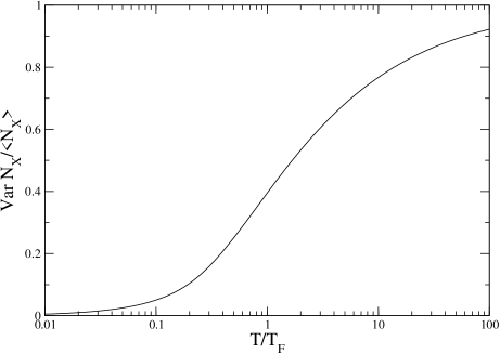
Figure 5: In the limit of a large interval of length $X$, ratio of the variance and the mean value of the number of impenetrable bosons in this interval, or equivalently of the number of fermions for an ideal Fermi gas, as function of the temperature in units of the Fermi temperature.

For a fixed temperature $T\ll T_{F}$, one can find the critical length $X_{c}$ below which the variance of the number of particles has the zero temperature behaviour Eq.(236) and above which it acquires the finite temperature behaviour Eq.(238). A first way of finding $X_{c}$ is to use Eq.(20) of [40] giving an approximation to the function $f(x)$ at $T\ll T_{F}$:

$$|f(x)|^{2}\simeq k_{F}^{2}\frac{T^{2}}{4T_{F}^{2}}\frac{\sin^{2}k_{F}x}{\sinh^{2}(\pi Tk_{F}x/2T_{F})}.$$ (242)

One sees that $f(x)$ differs weakly from its zero temperature value as long as $\pi Tk_{F}|x|\ll 2T_{F}$. One the contrary, if $\pi Tk_{F}|x|\gg 2T_{F}$, $|f(x)|^{2}$ is exponentially small so that one is left with Eq.(238). This gives a cross-over length

$$k_{F}X_{c}\sim\frac{2T_{F}}{\pi T}.$$ (243)

A second way of finding $X_{c}$ is to equate Eq.(236) and Eq.(238). Assuming $\ln 2k_{F}X_{c}\sim 1$, this gives the same order of magnitude for $X_{c}$ as in the previous equation. A third way is to imagine that one can introduce a fictitious box of size $X$ with periodic boundary conditions, containing a fictitious Fermi gas with the same chemical potential as the bulk system. This box gives wrong predictions at zero temperature, as the variance of $N_{X}$ would then be exactly zero, but gives indeed the correct result Eq.(238) for finite $T$, when the thermodynamic limit approximation is applicable for the fictitious box, which occurs when

$$k_{B}T>\Delta E$$ (244)

where $\Delta E$ is the energy separation between two consecutive energy levels in the box around the Fermi energy. One finds $\Delta E\sim 2\pi\hbar^{2}k_{F}/mX$ which leads to the same $X_{c}$ as before, within a numerical factor.

3.3 First order coherence function of impenetrable bosons

The first order coherence function in the general case of a spatially inhomogeneous system is defined as

$$g_{1}(x,y)=\langle\hat{\psi}^{\dagger}(y)\hat{\psi}(x)\rangle=\frac{1}{l}\langle\hat{a}^{\dagger}_{y}\hat{a}_{x}\rangle.$$ (245)

As the expectation value is taken over a density operator $\sigma$ such that ${\cal P}\sigma{\cal P}=\sigma$, one can add factors equal to ${\cal P}$ in the above expression. This leads to an expression for $g_{1}$ in terms of the fermionic operators:

$$g_{1}(x,y)=-l^{-1}\langle\hat{c}_{y}^{\dagger}\hat{c}_{x}e^{i\pi\sum_{z=x}^{y}\hat{c}_{z}^{\dagger}\hat{c}_{z}}\rangle$$ (246)

where we have assumed that $x<y$ [49].

We now go through a sequence of transformations of Eq.(246). First we rewrite it as

$$g_{1}(x,y)=-l^{-1}\frac{\mathrm{Tr}\left[\hat{c}_{y}^{\dagger}\hat{c}_{x}e^{A}e^{B}\right]}{\mathrm{Tr}\left[e^{B}\right]}$$ (247)

where $A$ and $B$ are operators that are quadratic in the fermionic variables. $B$ is equal to $-\beta\hat{H}_{\infty}$, where $\beta=1/k_{B}T$ and the Hamiltonian $\hat{H}_{\infty}$ is given by Eq.(226). The operator $A$ is $i\pi$ times the operator counting the number of fermions on the sites from $x$ to $y$. We introduce the matrices in the lattice basis of the one-body operators corresponding to $A$ and $B$:

$$A = \sum_{\alpha,\beta}{\cal A}_{\alpha\beta}\hat{c}^{\dagger}_{\alpha}\hat{c}_{\beta}$$ (248)

$$B = \sum_{\alpha,\beta}{\cal B}_{\alpha\beta}\hat{c}^{\dagger}_{\alpha}\hat{c}_{\beta}$$ (249)

Let us introduce a matrix ${\cal C}$ such that

$$e^{\cal A}e^{\cal B}=e^{\cal C}.$$ (250)

Then, as we show in the appendix 5, $e^{A}e^{B}=e^{C}$ where the operator $C$ is defined as

$$C=\sum_{\alpha,\beta}{\cal C}_{\alpha\beta}\hat{c}^{\dagger}_{\alpha}\hat{c}_{\beta}.$$ (251)

We also derive in this appendix the following expressions:

$$\frac{\mathrm{Tr}\left[\hat{c}_{y}^{\dagger}\hat{c}_{x}e^{C}\right]}{\mathrm{Tr}\left[e^{C}\right]}=\left(\frac{1}{1+e^{-{\cal C}}}\right)_{xy}.$$ (252)

$$\mathrm{Tr}\left[e^{C}\right]=\mathrm{det}\,(1+e^{\cal C}).$$ (253)

What remains to be done is to eliminate $\cal C$ in terms of $\cal A$ and $\cal B$: this is easy since $\cal C$ appears in the final result only through its exponential, so that Eq.(250) can be used directly. A further simplification arises from the fact that $\cal A$ is proportional to a projector. The calculations are detailed in the appendix, we give the result:

$$g_{1}(x,y)=\frac{1}{2l}\left(\frac{1}{1-2{\cal S}}\right)_{xy}\mathrm{det}(1-2{\cal S})\ \ \ \ \ \ \ \mathrm{for}\ \ \ x<y$$ (254)

where the matrix ${\cal S}$ is defined on the lattice sites in between $x$ and $y$ by the following thermal averages:

$$S_{\alpha\beta}\equiv\langle\hat{c}^{\dagger}_{\beta}\hat{c}_{\alpha}\rangle\ \ \ \ \ \mathrm{for}\ \ x\leq\alpha,\beta\leq y.$$ (255)

Interestingly, for the spatially homogeneous case, in the continuous limit $l\rightarrow 0$, where matrices are replaced by operators acting on a functional space and the dispersion relation for fermions is quadratic, Eq.(254) becomes formally equivalent to the expression of $g_{1}$ given in [50] for impenetrable bosons in the Lieb-Liniger model. In the general case, several equivalent forms of (254) can be obtained after simple linear algebra manipulations. First, using the matrix identity $M^{-1}={}^{t}\mathrm{com}\,M/\mathrm{det}\,M$ relating the inverse of a matrix $M$ to the transpose of its comatrix, we obtain:

$$g_{1}(x,y)=\frac{1}{2l}\mathrm{det}(2{\cal S}_{\alpha\beta}-\delta_{\alpha,\beta})|_{x\leq\alpha<y,x<\beta\leq y}\ \ \ \ \ \mathrm{for}\ \ x<y$$ (256)

that is in terms of the determinant of the matrix obtained by suppressing the first column and the last line of $2{\cal S}-1$. This coincides with [44] and, within a factor of two, with Eq.(8) of [40]. Second, introducing the one-fermion density operator $\hat{\sigma}$ such that $\langle z|\hat{\sigma}|z^{\prime}\rangle=\langle\hat{c}^{\dagger}_{z^{\prime}}\hat{c}_{z}\rangle/l$ due to the normalisation (135), and the single-particle orthogonal projector $\hat{\Pi}$ over the discrete position interval $x\leq z\leq y$, one gets the operatorial form $g_{1}(x,y)=\frac{1}{2}\langle x|(1-2\hat{\Pi}\hat{\sigma}\hat{\Pi})^{-1}|y\rangle\,\mathrm{det}(1-2\hat{\Pi}\hat{\sigma}\hat{\Pi})$ that can be rewritten as

$$g_{1}(x,y)=\langle x|\hat{\sigma}^{1/2}(1-2\hat{R})^{-1}\hat{\sigma}^{1/2}|y\rangle\,\mathrm{det}(1-2\hat{R})\ \ \ \ \ \mathrm{for}\ \ x<y$$ (257)

with $\hat{R}=\hat{\sigma}^{1/2}\hat{\Pi}\,\hat{\sigma}^{1/2}$. One has taken advantage of the identity

$$(1-2\hat{\Pi}\hat{\sigma}\hat{\Pi})^{-1}-1=2\hat{\Pi}\,\hat{\sigma}^{1/2}(1-2\hat{R})^{-1}\hat{\sigma}^{1/2}\hat{\Pi}$$ (258)

that results from a geometric series expansion and from $\hat{\Pi}^{2}=\hat{\Pi}$, $\hat{\sigma}^{1/2}(\hat{\Pi}\hat{\sigma}\hat{\Pi})^{n}\hat{\sigma}^{1/2}=\hat{R}^{n+1}$ $\forall n>0$. Similarly $\mathrm{Tr}[(\hat{\Pi}\hat{\sigma}\hat{\Pi})^{n}]=\mathrm{Tr}(\hat{R}^{n})$, so that $\mathrm{det}(1-2\hat{\Pi}\hat{\sigma}\hat{\Pi})=\mathrm{det}(1-2\hat{R})$ due the series expansion $\ln\mathrm{det}(1-\lambda M)=-\sum_{n\geq 1}\frac{\lambda^{n}}{n}\mathrm{Tr}(M^{n})$ valid for any matrix $M$. If one writes (257) in the eigenbasis of $\hat{\sigma}$, one obtains a finite temperature generalisation of [51]; this was pointed out to us by Yasar Atas and Isabelle Bouchoule, who obtained an independent derivation.

Extracting analytically physical information for $g_{1}$ is quite technical. The key result is the absence of long range order for the homogeneous system at zero temperature [52, 53]:

$$g_{1}(X)\sim\frac{A\rho}{|k_{F}X|^{1/2}}$$ (259)

where $A=0.92418\ldots$ is a numerical constant and $k_{F}X\gg 1$. We refer to [54] for an overview of the various analytical results. An important consequence of Eq.(259) is that the momentum distribution of impenetrable bosons at $T=0$, which is the Fourier transform of $g_{1}$, $\pi(k)=\int_{-\infty}^{+\infty}\cos(kx)g_{1}(x)$, diverges as $2A[k_{F}/(2\pi k)]^{1/2}$ when $k\rightarrow 0$.

In figure 6 is plotted the result of a calculation of $g_{1}(X)$ based on a numerical evaluation of the determinant in Eq.(256) at $T=0$. We have actually plotted the product of $g_{1}(X)$ with $(k_{F}X)^{1/2}$ to reveal that $g_{1}$ exhibits damped oscillations around the asymptotic formula Eq.(259): on a direct plot of the bare $g_{1}$, these oscillations are not visible in practice. Note that these oscillations have a maximum roughly at the half integer values of $\rho X$ and have a minimum roughly at the integer values of $\rho X$: this is in contradiction with the asymptotic series expansion of [53] but is reproduced by the analytical approach of [54].

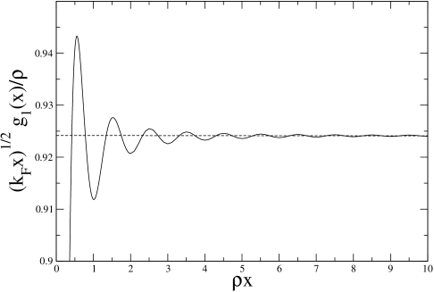
Figure 6: Coherence function $g_{1}(x)$ of a zero temperature spatially homogeneous gas of 1D impenetrable bosons in the thermodynamical limit, calculated numerically from Eq.(256), with $\rho l=0.005$. $g_{1}$ was multiplied by $(k_{F}x)^{1/2}$, where the Fermi wavevector $k_{F}$ is related to the density $\rho$ by $k_{F}=\pi\rho$, to reveal that $g_{1}$ oscillates around its asymptotic value. Dashed line: constant $A$ of Eq.(259).

Can we understand the emergence of such a $1/X^{1/2}$ asymptotic behaviour of $g_{1}$ at zero temperature ? We present here an interpretation with no pretension of rigor. The first step is to realize that the power law of the long range behavior of $g_{1}$ is not changed if one eliminates the factor $\hat{c}_{y}^{\dagger}\hat{c}_{x}/l$ in the Eq.(246). This is suggested by the calculations of [44], and we have checked this fact numerically. What remains to be understood is the long range behaviour of the function

$$G(X)\equiv\langle e^{i\pi\hat{N}_{X}}\rangle=\sum_{n=0}^{+\infty}\pi_{n}e^{i\pi n}$$ (260)

where $\hat{N}_{X}=\sum_{z=0}^{X}\hat{c}^{\dagger}_{z}\hat{c}_{z}$ is the operator giving the number of particles in the considered interval of length $X$, and $\pi_{n}$ is the probability of having $n$ particles in the interval. $G(X)$ is then the difference of the probability of having an even number of particles and the probability of having an odd number of particles in the interval. This can be estimated heuristically by assuming that the probability distribution of the number of fermions in the interval is roughly Gaussian for $k_{F}X\gg 1$ [55]. One can then extend the summation for $n$ to $-\infty$ since the standard deviation $\sigma_{X}$ of the Gaussian, while being much larger than unity, is much smaller than the mean of the Gaussian. Using the Poisson formula

$$\sum_{n=-\infty}^{+\infty}f(n)=\sum_{n=-\infty}^{+\infty}\tilde{f}(2\pi n)$$ (261)

where $\tilde{f}(k)=\int dxf(x)\exp(-ikx)$ is the Fourier transform of an arbitrary function $f(x)$, and restricting in the right hand side sum to the leading terms with $n=0$ and $n=1$, one obtains

$$G(X)\simeq 2\cos(\pi\rho X)e^{-\pi^{2}\sigma_{X}^{2}/2}.$$ (262)

The expression Eq.(236) of the standard deviation in the large $X$ limit leads to

$$G(X)\simeq\frac{0.36}{(\rho X)^{1/2}}\cos(\pi\rho X).$$ (263)

A numerical calculation confirms this result, with a coefficient $0.33$ rather than $0.36$.

The conclusion is that the $1/X^{1/2}$ behaviour of the first order coherence function in the ground state of impenetrable bosons in 1D reflects a property of the counting statistics of a 1D zero temperature ideal Fermi gas in an interval of length $X$.

4 Wick’s theorem

Consider the following problem: for a density operator (here for bosons for simplicity, we shall come to the case of fermions later)

$$\rho=\frac{1}{Z}\exp\left[-\sum_{\alpha}\nu_{\alpha}\hat{a}_{\alpha}^{\dagger}\hat{a}_{\alpha}\right]$$ (264)

where all $\nu_{\alpha}$ are strictly positive, and the $\hat{a}_{\alpha}$’s obey bosonic commutation relations:

$$[\hat{a}_{\alpha},\hat{a}_{\beta}^{\dagger}]=\delta_{\alpha\beta}$$ (265)

$$[\hat{a}_{\alpha},\hat{a}_{\beta}]=0,$$ (266)

calculate the expectation value

$$I=\langle\hat{b}_{1}\ldots\hat{b}_{2n}\rangle\equiv\mbox{Tr}\left[\hat{b}_{1}\ldots\hat{b}_{2n}\frac{1}{Z}e^{-\sum_{\alpha}\nu_{\alpha}\hat{a}_{\alpha}^{\dagger}\hat{a}_{\alpha}}\right]$$ (267)

where the $\hat{b}_{i}$’s are arbitrary linear combinations of $\hat{a}_{\alpha}$’s and $\hat{a}_{\alpha}^{\dagger}$’s. We consider an even number of factors as the expectation value of the product of an odd number of $\hat{b}$’s vanishes.

A physical example is simply the ideal Bose gas at thermal equilibrium in the grand canonical ensemble, with $\nu_{\alpha}=\beta(\epsilon_{\alpha}-\mu)$. Note that the density operator in the canonical ensemble does not reduce to (264) as it involves in addition the projector $P_{N}$ on the subspace with a fixed total number of particles equal to $N$.

The explicit calculation proceeds in four steps, in a derivation inspired by the lectures on statistical physical of Jacques des Cloizeaux at the Ecole normale supérieure of Paris, France, in 1988.

First step: assume that $\hat{b}_{1}$ is either $\hat{a}_{\alpha_{0}}$ or $\hat{a}_{\alpha_{0}}^{\dagger}$. Then there exists a number $\lambda$ such that

$$\hat{\rho}\hat{b}_{1}=\lambda\hat{b}_{1}\hat{\rho}.$$ (268)

One can check this identity using the Fock basis. E.g. one finds $\lambda=\exp\nu_{\alpha_{0}}$ for $\hat{b}_{1}=\hat{a}_{\alpha_{0}}$. By using the invariance of the trace by a cyclic permutation of the operators, one transfers $\hat{b}_{1}$ to the extreme right and one then puts it through $\hat{\rho}$ thanks to (268):

$$\langle\hat{b}_{1}\ldots\hat{b}_{2n}\rangle=\lambda\langle\hat{b}_{2}\ldots\hat{b}_{2n}\hat{b}_{1}\rangle.$$ (269)

The following commutation relation allows to reintegrate the factor $\hat{b}_{1}$ in the extreme left:

$$[\hat{b}_{1},\hat{b}_{2}\ldots\hat{b}_{2n}]=\sum_{j=2}^{2n}\hat{b}_{1}\ldots\hat{b}_{j-1}[\hat{b}_{1},\hat{b}_{j}]\hat{b}_{j+1}\ldots\hat{b}_{2n}.$$ (270)

Since the commutator of two $\hat{b}$’s is a pure number, we obtain

$$\langle\hat{b}_{1}\ldots\hat{b}_{2n}\rangle=\sum_{j=2}^{2n}\frac{[\hat{b}_{1},\hat{b}_{j}]}{\lambda-1}\langle\hat{b}_{2}\ldots\hat{b}_{j-1}\hat{b}_{j+1}\ldots\hat{b}_{2n}\rangle.$$ (271)

Second step: Apply this general formula for two operators:

$$\langle\hat{b}_{1}\hat{b}_{j}\rangle=\frac{[\hat{b}_{1},\hat{b}_{j}]}{\lambda-1}.$$ (272)

This identity, which in particular implies the Bose formula, allows to rewrite the general formula in a simpler way, without any apparition of $\lambda$:

$$\langle\hat{b}_{1}\ldots\hat{b}_{2n}\rangle=\sum_{j=2}^{2n}\langle\hat{b}_{1}\hat{b}_{j}\rangle\langle\hat{b}_{2}\ldots\hat{b}_{j-1}\hat{b}_{j+1}\ldots\hat{b}_{2n}\rangle.$$ (273)

Third step: the linearity of (273) with respect to $\hat{b}_{1}$ implies that it holds even if $\hat{b}_{1}$ is an arbitrary linear combination of $\hat{a}_{\alpha}$’s and $\hat{a}_{\alpha}^{\dagger}$’s!

Fourth step: iterate the formula (273) down to $2n=2$. So the most general expectation value $I$ can be expressed in terms of expectation values of binary products, which are of course known from the Bose formula.

The result is found to have a simple structure if one introduces the concept of a contraction. One collects the first factor $\hat{b}_{1}$ with one of the other factors, that we call $\hat{b}_{\alpha}$: one says that one performs a contraction of $\hat{b}_{1}$ with $\hat{b}_{\alpha}$. One contracts the next factor available, $\hat{b}_{\beta}$, with one of the factors left, $\hat{b}_{\gamma}$. Note that $\hat{b}_{\beta}=\hat{b}_{2}$ if $\alpha\neq 2$, otherwise $\beta=3$. One repeats this process until all the factors are contracted. Then

$$\langle\hat{b}_{1}\ldots\hat{b}_{2n}\rangle=\sum_{\rm all\ contractions}\langle\hat{b}_{1}\hat{b}_{\alpha}\rangle\langle\hat{b}_{\beta}\hat{b}_{\gamma}\rangle\ldots\langle\hat{b}_{\psi}\hat{b}_{\omega}\rangle.$$ (274)

Let us count the number of possible ways of contracting the $2n$ factors. There are $2n-1$ possibilities for the choice of the companion of $\hat{b}_{1}$, that is for the choice of $\hat{b}_{\alpha}$. There are $2n-3$ possibilities for the choice of the companion of $\hat{b}_{\beta}$, that is for the choice of $\hat{b}_{\gamma}$… Finally, there is a single possibility for the choice of the companion of $\hat{b}_{\psi}$, that is for the choice of $\hat{b}_{\omega}$. The total number of possible contractions is therefore

$$(2n-1)\times(2n-3)\times\ldots\times 1=\frac{(2n)!}{2^{n}n!}.$$ (275)

Let us give an example for $n=2$:

$$\langle\hat{b}_{1}\hat{b}_{2}\hat{b}_{3}\hat{b}_{4}\rangle=\langle\hat{b}_{1}\hat{b}_{2}\rangle\langle\hat{b}_{3}\hat{b}_{4}\rangle+\langle\hat{b}_{1}\hat{b}_{3}\rangle\langle\hat{b}_{2}\hat{b}_{4}\rangle+\langle\hat{b}_{1}\hat{b}_{4}\rangle\langle\hat{b}_{2}\hat{b}_{3}\rangle.$$ (276)

What happens for fermions? The annihilation and creation operators now obey anticommutation relations

$$\{\hat{a}_{\alpha},\hat{a}_{\beta}^{\dagger}\} = \delta_{\alpha\beta}$$ (277)

$$\{\hat{a}_{\alpha},\hat{a}_{\beta}\} = 0.$$ (278)

As the number operator $\hat{a}_{\alpha}^{\dagger}\hat{a}_{\alpha}$ is now bounded from above by unity, the coefficient $\nu_{\alpha}$ is no longer restricted to positive values. The same technique as for bosons can be applied to derive the following recursive relation:

$$\langle\hat{b}_{1}\ldots\hat{b}_{2n}\rangle=\sum_{j=2}^{2n}(-1)^{j}\langle\hat{b}_{1}\hat{b}_{j}\rangle\langle\hat{b}_{2}\ldots\hat{b}_{j-1}\hat{b}_{j+1}\ldots\hat{b}_{2n}\rangle.$$ (279)

The factor $(-1)^{j}$ appears because $\hat{b}_{j}$ ‘crossed’ $j-2$ factors. This gives rise to the Wick’s rule:

$$\langle\hat{b}_{1}\ldots\hat{b}_{2n}\rangle=\sum_{\rm all\,contractions}\epsilon_{\rm contraction}\langle\hat{b}_{1}\hat{b}_{\alpha}\rangle\langle\hat{b}_{\beta}\hat{b}_{\gamma}\rangle\ldots\langle\hat{b}_{\psi}\hat{b}_{\omega}\rangle.$$ (280)

A sign $\pm$, that we denote as $\epsilon_{\rm contraction}$, is associated to each contraction. Each contraction actually defines a permutation of the $2n$ factors, performing the following mapping:

$$(1,2,3,4,\ldots,2n-1,2n)\rightarrow(1,\alpha,\beta,\gamma,\ldots,\psi,\omega).$$ (281)

$\epsilon_{\rm contraction}$ is simply the signature of this permutation, that is $(-1)$ to the power the number of transpositions of two elements required to realize the permutation. Let us give an example for $n=2$:

$$\langle\hat{b}_{1}\hat{b}_{2}\hat{b}_{3}\hat{b}_{4}\rangle=\langle\hat{b}_{1}\hat{b}_{2}\rangle\langle\hat{b}_{3}\hat{b}_{4}\rangle-\langle\hat{b}_{1}\hat{b}_{3}\rangle\langle\hat{b}_{2}\hat{b}_{4}\rangle+\langle\hat{b}_{1}\hat{b}_{4}\rangle\langle\hat{b}_{2}\hat{b}_{3}\rangle.$$ (282)

5 Some useful identities for Gaussian operators

Consider operators $A$, $B$ and $C$ that are quadratic in the fermionic field, in the sense defined by Eq.(248,249,251). The square matrices $\cal A$, $\cal B$ and $\cal C$ of the associated quadratic forms are linked by Eq.(250).

5.1 $ABC$ identity

We prove that the identity $e^{A}e^{B}=e^{C}$ holds. The idea of the proof is to consider each exponential factor as an evolution operator and to show that the composition of two Gaussian evolution operators gives a Gaussian evolution operator.

Let us introduce the formal time evolution:

$$\hat{c}_{\alpha}(\tau)\equiv e^{\tau B}\hat{c}_{\alpha}e^{-\tau B}.$$ (283)

The time derivative of $\hat{c}_{\alpha}(\tau)$ involves the commutator of $B$ and $\hat{c}_{\alpha}$ that can be calculated from the fermionic anticommutation relations:

$$\frac{d}{d\tau}\hat{c}_{\alpha}(\tau)=-\sum_{\beta}{\cal B}_{\alpha\beta}\hat{c}_{\beta}(\tau).$$ (284)

This differential system with the initial conditions $\hat{c}_{\alpha}(0)=\hat{c}_{\alpha}$ is integrated formally in terms of the evolution matrix $e^{-{\cal B}\tau}$. Specializing to $\tau=1$ we obtain

$$e^{B}\hat{c}_{\alpha}e^{-B}=\sum_{\beta}\left(e^{-{\cal B}}\right)_{\alpha\beta}\hat{c}_{\beta}.$$ (285)

By using the same type of identity with $B$ replaced with $A$ or with $C$ we obtain

$$e^{A}e^{B}\hat{c}_{\alpha}e^{-B}e^{-A} = \sum_{\beta,\gamma}\left(e^{-{\cal B}}\right)_{\alpha\beta}\left(e^{-{\cal A}}\right)_{\beta\gamma}\hat{c}_{\gamma}$$ (286)

$$= \sum_{\gamma}\left(e^{-{\cal B}}e^{-{\cal A}}\right)_{\alpha\gamma}\hat{c}_{\gamma}=\sum_{\gamma}\left(e^{-{\cal C}}\right)_{\alpha\gamma}\hat{c}_{\gamma}$$ (287)

$$= e^{C}\hat{c}_{\alpha}e^{-C}$$ (288)

where we used Eq.(250). Similarly one can show that

$$e^{A}e^{B}\hat{c}_{\alpha}^{\dagger}e^{-B}e^{-A}=e^{C}\hat{c}_{\alpha}^{\dagger}e^{-C}.$$ (289)

Consider now the action of $e^{C}$ on an Hartree-Fock state defined by an arbitrary list $\gamma_{1},\ldots,\gamma_{n}$ of single particle states:

$$|\psi\rangle\equiv\hat{c}_{\gamma_{1}}^{\dagger}\ldots\hat{c}_{\gamma_{n}}^{\dagger}|0\rangle.$$ (290)

We perform the following sequence of transformations:

$$e^{C}|\psi\rangle = \left(e^{C}\hat{c}_{\gamma_{1}}^{\dagger}e^{-C}\right)\ldots\left(e^{C}\hat{c}_{\gamma_{n}}^{\dagger}e^{-C}\right)|0\rangle$$ (291)

$$= \left(e^{A}e^{B}\hat{c}_{\gamma_{1}}^{\dagger}e^{-B}e^{-A}\right)\ldots\left(e^{A}e^{B}\hat{c}_{\gamma_{n}}^{\dagger}e^{-B}e^{-A}\right)|0\rangle$$ (292)

$$= e^{A}e^{B}|\psi\rangle$$ (293)

where we used the fact that $e^{-C}|0\rangle=e^{-B}|0\rangle=e^{-A}|0\rangle=|0\rangle$ as can be checked by the power series expansion of the exponential. The operators $e^{C}$ and $e^{A}e^{B}$ have the same action on all the Hartree-Fock states, which form a basis, so they are equal.

5.2 Trace and one-body expectation values of a Gaussian operator

What is the trace of $e^{C}$ ? What is the one-body operator corresponding to $e^{C}$ ? We give the answer assuming that the matrix $\cal C$ is diagonalizable, which is sufficient to conclude in the general case using a continuity argument.

We call $e_{i}$ the set of eigenvectors of $\cal C$, with eigenvalue ${\cal C}_{i}$, so that ${\cal C}e_{i}={\cal C}_{i}e_{i}$, and we call $f_{j}$ the adjoint basis normalized such that

$$f_{j}^{*}\cdot e_{i}=\delta_{i,j}$$ (294)

so that the closure relation is satisfied:

$$\sum_{i}(e_{i})_{\alpha}(f_{i})^{*}_{\beta}=\delta_{\alpha,\beta}$$ (295)

where $(e_{i})_{\alpha}$ is the component of the vector $e_{i}$ in the original single particle basis.

We introduce the corresponding creation and annihilation operators:

$$\hat{b}_{i} \equiv \sum_{\alpha}\hat{c}_{\alpha}(f_{i})_{\alpha}^{*}$$ (296)

$$\hat{b}_{i}^{+} \equiv \sum_{\alpha}\hat{c}_{\alpha}^{\dagger}(e_{i})_{\alpha}.$$ (297)

Note that in general the creation operator $\hat{b}_{i}^{+}$ is not the Hermitian conjugate of the annihilation operator $\hat{b}_{i}$ since the matrix $\cal C$ is not necessarily Hermitian. This is why we introduced the symbol $+$ rather than $\dagger$ in the exponent. However this has little effect on the algebra of second quantization! The $\hat{b}_{i}$’s obviously anticommute among themselves, since they are linear combinations of the $\hat{c}_{\alpha}$’s; also, their action on vacuum on the right gives zero. Similarly, the $\hat{b}_{i}^{+}$’s anticommute among themselves and their action on vacuum on the left gives zero. Finally, one derives from Eq.(294) the anticommutation relations

$$\{\hat{b}_{i},\hat{b}_{j}^{+}\}=\delta_{i,j}.$$ (298)

We can then construct a Fock basis as

$$|\{n\}\rangle\equiv\left(b_{1}^{+}\right)^{n_{1}}\ldots\left(b_{M}^{+}\right)^{n_{M}}|0\rangle$$ (299)

where $M$ is the order of the matrix $\cal C$, that is the dimension of the single particle state space, and the occupation numbers $n_{i}$ are equal to 0 or 1. The adjoint Fock basis is

$$\overline{\langle\{n\}|}\equiv\langle 0|\left(b_{M}\right)^{n_{M}}\ldots\left(b_{1}\right)^{n_{1}}.$$ (300)

The advantage of these algebraic constructions is that the operator $C$ has now simple expressions and actions:

$$C=\sum_{i}{\cal C}_{i}\hat{b}_{i}^{+}\hat{b}_{i}$$ (301)

and, from the usual calculus in second quantized form:

$$C|\{n\}\rangle=\left(\sum_{i}{\cal C}_{i}n_{i}\right)|\{n\}\rangle.$$ (302)

As a consequence

$$\mbox{Tr}\,\left[e^{C}\right]=\sum_{\{n\}}\prod_{i}e^{n_{i}{\cal C}_{i}}=\mathrm{det}\,\left(1+e^{\cal C}\right).$$ (303)

One has also

$$\frac{\mbox{Tr}\,\left[\hat{b}_{i}^{+}\hat{b}_{j}e^{C}\right]}{\mbox{Tr}\,\left[e^{C}\right]}=\delta_{i,j}\frac{1}{1+e^{-{\cal C}_{i}}}$$ (304)

and finally, using the closure relation Eq.(295), we get Eq.(252).

5.3 Back to $g_{1}$

We assume now that the matrix $\cal A$ takes the specific form $i\pi{\cal Q}$ where the matrix ${\cal Q}$ is a projector on the sites in between $x$ and $y$:

$${\cal Q}_{\alpha\beta}=\delta_{\alpha,\beta}\sum_{z=x}^{y}\delta_{\alpha,z}.$$ (305)

This leads to strong simplifications. First one has

$$e^{\cal A}=1-2{\cal Q}.$$ (306)

So, from Eq.(250):

$$1+e^{\cal C}=1+(1-2{\cal Q})e^{\cal B}=\left[1-2{\cal Q}{\cal S}\right](1+e^{\cal B})$$ (307)

where we have introduced

$${\cal S}\equiv\frac{1}{1+e^{-{\cal B}}}.$$ (308)

This last matrix has a very simple physical interpretation: using Eq.(252) with $C$ replaced by $B$, we find that ${\cal S}_{\alpha\beta}$ is the thermal average of $\hat{c}_{\beta}^{\dagger}\hat{c}_{\alpha}$. We finally obtain

$$\frac{1}{1+e^{-{\cal C}}}=e^{\cal C}\frac{1}{1+e^{\cal C}}=(1-2{\cal Q}){\cal S}\frac{1}{1-2{\cal Q}{\cal S}}.$$ (309)

The matrix to invert in the above expression can be put in block triangular form by collecting the lattice sites in between $x$ and $y$ in one block, and the other lattice sites in a second block. In block notations, one can check that

$$\left(\begin{array}[]{cc}\mathrm{block}_{11}&\mathrm{block}_{12}\\ 0&\mathrm{block}_{22}\end{array}\right)^{-1}=\left(\begin{array}[]{cc}\mathrm{block}_{11}^{-1}&-\mathrm{block}_{11}^{-1}\,\mathrm{block}_{12}\,\mathrm{block}_{22}\\ 0&\mathrm{block}_{22}^{-1}\end{array}\right).$$ (310)

Here the right upper block of the inverse matrix is not useful as the lattice site $y$, on which the inverse matrix acts in the expression for $g_{1}(x,y)$, belongs to the first block. One has also that the determinant of a block triangular matrix is the product of the determinants of block₁₁ and block₂₂. This leads to

$$g_{1}(x,y)=\frac{1}{2l}\left[-\delta_{x,y}+\left(\frac{\cal Q}{{\cal Q}-2{\cal Q}{\cal S}{\cal Q}}\right)_{x,y}\right]\mathrm{det}\,\left[{\cal Q}-2{\cal Q}{\cal S}{\cal Q}\right].$$ (311)

When specialized to the case $x\neq y$, this gives Eq.(254).

References

- [1] Y. Castin, p.1-136, in Coherent atomic matter waves, Lecture notes of Les Houches summer school, edited by R. Kaiser, C. Westbrook, and F. David, EDP Sciences and Springer-Verlag (2001).
- [2] B. Diu, C. Guthman, D. Lederer, and B. Roulet, Physique Statistique (Hermann, Paris, France, 1989).
- [3] M. Holthaus, E. Kalinowski, “The saddle-point method for condensed Bose gases”, Ann. Phys. (N.Y.) 276, 321 (1999).
- [4] A. Sinatra, C. Lobo, Y. Castin, “The truncated Wigner method: limits of validity and applications”, J. Phys. B 35, 3599-3631 (2002).
- [5] E. H. Lieb and W. Liniger, “Exact Analysis of an Interacting Bose Gas. I. The General Solution and the Ground State”, Phys. Rev. 130, 1605 (1963).
- [6] C.N. Yang, C.P. Yang, “Thermodynamics of a one-dimensional system of bosons with repulsive delta-function interaction”, J. Math. Phys. 10, 1115 (1969).
- [7] M. Gaudin, La fonction d’onde de Bethe, Masson (Paris, 1983).
- [8] Y. Castin, C. Herzog, “Bose-Einstein condensates in symmetry breaking states”, Comptes Rendus de l’Académie des Sciences de Paris, tome 2, série IV, p.419-443 (2001).
- [9] K.V. Kheruntsyan, D.M. Gangardt, P.D. Drummond, and G.V. Shlyapnikov, “Pair Correlations in a Finite-Temperature 1D Bose Gas”, Phys. Rev. Lett. 91, 040403 (2003).
- [10] D.J. Scalapino, M. Sears, R.A. Ferrell, “Statistical Mechanics of One-Dimensional Ginzburg-Landau Fields”, Phys. Rev. B 6, 3409 (1972).
- [11] Y. Castin, R. Dum, E. Mandonnet, A. Minguzzi and I. Carusotto, “Coherence properties of a continuous atom laser”, Journal of Modern Optics 47, 2671-2695 (2000).
- [12] C. Gardiner, Quantum Noise, Springer-Verlag Berlin Heidelberg (1991), chapter 4 “Phase space methods”.
- [13] Note that the normalization factor of is infinite for a system with an infinite number of modes. This formal problem is solved by the introduction of an energy cut-off that one puts to infinity at the end of the calculations.
- [14] Yu. Kagan and B. Svistunov, ‘Evolution of Correlation Properties and Appearance of Broken Symmetry in the Process of Bose-Einstein Condensation’, Phys. Rev. Lett. 79, 3331 (1997) and references therein.
- [15] V. A. Kashurnikov, N. V. Prokof’ev, and B. V. Svistunov, “Critical Temperature Shift in Weakly Interacting Bose Gas”, Phys. Rev. Lett. 87, 120402 (2001).
- [16] P. Arnold, G. Moore, “BEC Transition Temperature of a Dilute Homogeneous Imperfect Bose Gas”, Phys. Rev. Lett. 87, 120401 (2001).
- [17] We recall that a functional integral is defined as a limit of a discrete representation. Here, one should first discretize the ‘time’ with a step , and then take the limit . This implies that the Laplacian in the energy functional should be considered as the limit of a discrete Laplacian, e.g. with the usual 3-point formula. The cyclic boundary condition for the discrete Laplacian ensures that its eigenmodes at a given energy are two counterpropagating plane waves. This would not be the case for the continuous Laplacian, in the absence of the extra condition .
- [18] V. N. Popov, Functional Integrals in Quantum Field Theory and Statistical Physics, (Reidel, Dordrecht, 1983).
- [19] More rigorously, one has also to perform a sum over all possible winding numbers of the field. In the thermodynamic limit this has no effect on observables like the first order or second order correlation functions considered here, but it has a dramatic effect on the superfluid fraction, see [20, 21]
- [20] N. V. Prokof’ev and B. V. Svistunov, “Two Definitions of Superfluid Density”, Phys. Rev. B 61, 11282 (2000).
- [21] I. Carusotto, Y. Castin, “Superfluidity of the 1D Bose gas”, C. R. Physique 5, 107-127 (2004).
- [22] We have discovered a posteriori that such a proof of non-existence for continuous bosonic fields was available in the literature, see H. Fröhlich, Physica 34, 47 (1967).
- [23] M. Girardeau and R. Arnowitt, “Theory of Many-Boson Systems: Pair Theory”, Phys. Rev. 113, 755 (1959).
- [24] Y. Castin and R. Dum, “Low temperature Bose-Einstein condensates in time dependent traps: beyond the -symmetry breaking approach”, Phys. Rev. A 57, 3008-3021 (1998).
- [25] S.M. Barnett, and D.C. Pegg, “The Hermitian Optical Phase Operator”, in S. Reynaud, E. Giacobino and J. Zinn-Justin, editors, Fluctuations Quantiques, école d’été des Houches 1995, p. 563 (Elsevier, 1997).
- [26] R. Newton, Scattering Theory of Waves and Particles, Dover (2003).
- [27] In particular, there is no relation between , and .
- [28] C. Mora, Y. Castin, “Extension of Bogoliubov theory to quasicondensates”, Phys. Rev. A 67, 053615 (2003).
- [29] R. Combescot, “Feshbach Resonance in Dense Ultracold Fermi Gases”, Phys. Rev. Lett. 91, 120401 (2003).
- [30] M. Olshanii, “Atomic Scattering in the Presence of an External Confinement and a Gas of Impenetrable Bosons”, Phys. Rev. Lett. 81, 938-941 (1998).
- [31] T. Bergeman, M. G. Moore, and M. Olshanii, “Atom-Atom Scattering under Cylindrical Harmonic Confinement: Numerical and Analytic Studies of the Confinement Induced Resonance”, Phys. Rev. Lett. 91, 163201 (2003).
- [32] J.P. Blaizot, G. Ripka, Quantum Theory of Finite Systems (The MIT Press, 1985).
- [33] M. Lewenstein, Li You, “Quantum Phase Diffusion of a Bose-Einstein Condensate”, Phys. Rev. Lett. 77, 3489 (1996).
- [34] The first term in the right hand side of this expression should not be forgotten, e.g. in symmetry breaking Bogoliubov approaches, as emphasized in [32], Eq.(3.48). We have used the identity to obtain it, see Eq.(105) of [28].
- [35] V. N. Popov, “Long-wave asymptotic form of the many-body Green’s functions of a one-dimensional Bose gas”, JETP Lett. 31, 526 (1980).
- [36] M. Schwartz, “Off-diagonal long-range behaviour of interacting Bose systems”, Phys. Rev. B 15, 1399 (1977).
- [37] The estimate given in [28] that this distance is the largest of the two distances and is actually wrong.
- [38] C. Mora, thèse de doctorat de l’Université Paris 6 (2003), published on http://ccsd.cnrs.fr
- [39] M. Olshanii, V. Dunjko, “Short distance correlation properties of the Lieb-Liniger system and momentum distributions of trapped one-dimensional atomic gases”, Phys. Rev. Lett. 91, 090401 (2003).
- [40] K.B. Efetov, A. I. Larkin, “Correlation functions in one-dimensional systems with a strong interaction”, Sov. Phys. JETP 42, 390 (1976).
- [41] F.D.M. Haldane, “Effective harmonic-fluid approach to low-energy properties of one-dimensional quantum fluids”, Phys. Rev. Lett. 47, 1840 (1981).
- [42] In practice it is difficult to exactly satisfy this condition. One may consider the 1D coupling constant to be infinite if, for the maximum wavevector relevant in the physical state, the scattering amplitude is very close to the one of the infinite delta. This implies , see Eq.(158).
- [43] M. Girardeau, “Relationship between Systems of Imepenetrable Bosons and Fermions in One Dimension”, J. Math. Phys. 1, 516 (1960).
- [44] T.D. Schultz, “Note on the One-Dimensional Gas of Impenetrable Point-Particle Bosons”, J. Math. Phys. 4, 666 (1963).
- [45] M. A. Cazalilla, “One-dimensional optical lattices and impenetrable bosons”, Phys. Rev. A 67, 053606 (2003).
- [46] In the case where the trapping potential is replaced by periodic boundary conditions on the bosons with spatial period , the point of the grid of position is identified with the point of position , so that . In the fermionic counterpart one finds that where gives the total number of particles. The boundary conditions for the fermions are therefore periodic for odd or antiperiodic for even. We shall ignore here such point, as the numerical examples to come correspond to the thermodynamic limit. This point may become important for finite size systems, and it is explained in an appendix of [47] how to deal with it analytically.
- [47] I. Carusotto, Y. Castin, “An exact reformulation of the Bose-Hubbard model in terms of a stochastic Gutzwiller ansatz”, New Journal of Physics 5, 91.1-91.13 (2003).
- [48] As the coefficient of is positive, the variance is a convex function of temperature at . As the variance tends to one at large temperature, it necessarily presents an inflexion point, that we find numerically to be at .
- [49] If , one may use the relation .
- [50] V.E. Korepin, N.M. Bogoliubov and A.G. Izergin, “Quantum Inverse Scattering Method and Correlation Functions”, (Cambridge University Press 1993).
- [51] R. Pezer and H. Buljan, “Momentum Distribution Dynamics of a Tonks-Girardeau Gas: Bragg Reflections of a Quantum Many-Body Wave Packet”, Phys. Rev. Lett. 98, 240403 (2007).
- [52] A. Lenard, “Momentum distribution in ground state of 1-dimensional system of impenetrable bosons”, J. Math. Phys. 5, 930 (1964); “One-dimensional impenetrable bosons in thermal equilibrium”, J. Math.Phys. 7, 1268 (1966).
- [53] H.G. Vaidya and C.A. Tracy, “One-Particle Reduced Density Matrix of Impenetrable Bosons in One Dimension at Zero Temperature”, Phys. Rev. Lett. 42, 3 (1979) and J. Math. Phys. 20, 2291 (1979).
- [54] D. Gangardt, “Universal correlations of trapped one-dimensional impenetrable bosons”, J. Phys. A 37, 9335 (2004).
- [55] It is shown with the bozonisation technique that the distribution is indeed Gaussian in the large limit: see the paragraph below Eq.(31) in the paper by L. S. Levitov, H.-W. Lee, and G. B. Lesovik, J. Math. Phys. 37, 4845 (1996).