The treatment of zero eigenvalues of the matrix governing the equations of motion in
many-body Green’s function theory.

Abstract

The spectral theorem of many-body Green’s function theory relates thermodynamic correlations to Green’s functions. More often than not, the matrix $\mathbf{\Gamma}$ governing the equations of motion has zero eigenvalues. In this case, the standard text-book approach requires both commutator and anti-commutator Green’s functions to obtain equations for that part of the correlation which does not lie in the null space of the matrix. In this paper, we show that this procedure fails if the projector onto the null space is dependent on the momentum vector, $\bf k$. We propose an alternative formulation of the theory in terms of the non-null space alone and we show that a solution is possible if one can find a momentum-independent projector onto some subspace of the non-null space. To do this, we enlist the aid of the singular value decomposition (SVD) of $\mathbf{\Gamma}$ in order to project out the null space, thus reducing the size of the matrix and eliminating the need for the anti-commutator Green’s function. We extend our previous workFK03 , dealing with a ferromagnetic Heisenberg monolayer and a momentum-independent projector onto the null space, to models where both multilayer films and a momentum-dependent projector are considered. We develop the numerical methods capable of handling these cases and offer a computational algorithm that should be applicable to any similar problem arising in Green’s function theory.

I Introduction

The spectral theorem in many-body Green’s function (GF) theory relates thermodynamic correlations to Green’s functions, thus providing equations which, when iterated to self-consistency, allow the computation of the expectation values of the operators from which the Green’s functions are constructed. Each Green’s function can be expressed in terms of an inhomogeneity of the equations of motion and higher-order Green’s functions. Each higher-order GF can in turn be expressed in terms of yet another inhomogeneity and even higher-order Green’s functions, and so on. Truncation of this infinite, exact hierarchy seldom occurs naturally. It is usually brought about through a decoupling approximation, whereby the GFs of some order are approximated as linear combinations of lower-order functions which have already appeared in the hierarchy. This leads to a closed system of linear equations, the so-called equations of motion, which relate the Green’s functions to the inhomogeneities. Anticipating results from the detailed exposition in the next section, we may write the equation of motion in compact matrix notation:

$$(\omega{\bf 1}-{\bf\Gamma}){\bf G}={\bf A}.$$ (1)

Here, $\bf G$ is a vector whose components are the Green’s functions, $\bf A$ is a vector of associated inhomogeneities, and $\mathbf{\Gamma}$ is the matrix (in general unsymmetric) containing the coefficients obtained via the truncation.

Each Green’s function has poles at all the eigenvalues, $\omega_{i}$, of the matrix $\mathbf{\Gamma}$. As we shall show in detail in the overview section below, the spectral theorem associates a vector of correlation functions, $\bf C$, to quantities at these poles, and thereby provides a route from the inhomogeneity vector to the vector of correlation functions. In fact, this relationship can be expressed compactlyFJKE00 by a multiplication of the vector $\bf A$ by a matrix constructed from the eigenvalues, $\omega_{i}$, and the right and left matrices of eigenvectors, $\bf R,L$ of the matrix $\mathbf{\Gamma}$:

$$\bf C = {\bf R}{\cal E}\bf LA,$$ (2)

$${\bf L}{\mathbf{\Gamma}}{\bf R} = {\mathbf{\Omega}},$$ (3)

where $\bf\Omega$ is a diagonal matrix having the eigenvalues $\omega_{i}$ on the principal diagonal and $\cal E$ is a related diagonal matrix with elements ${\cal E}_{ij}=\delta_{ij}/(e^{\beta\omega_{i}}-1)\$, $\beta$ being $1/(kT)$. Since $\bf C$, $\bf A$, and $\mathbf{\Gamma}$ all depend on the set of expectation values of the operators used in constructing the Green’s functions, Eq. 2 can be solved by varying the expectation values until the left and right hand sides of the equation are equal. Usually, the equation holds in momentum space, so a Fourier transform to coordinate space (an integration over the momentum $\bf k$) is also required; i.e. a set of integral equations has to be solved self-consistently.

This procedure, while somewhat complicated to derive, is straightforward to apply, unless, as very often happens, the matrix $\mathbf{\Gamma}$ has a null space, i.e. there are eigenvalues of value zero. In that case, a naive use of Eq. 2 would involve a division by zero in the evaluation of $\cal E$. The standard textbook procedure for handling the null space demands a knowledge of the anti-commutator GF in addition to the commutator GF from which Eq. 2 was derived (see references ST65 ; RG71 and textbooks Nol86 ; GHE01 ). This leads to additional terms in Eq. 2 which restrict the GF method to the evaluation not of the complete vector $\bf C$, but only to that part of $\bf C$ which lies in the non-null space of the matrix $\mathbf{\Gamma}$. While this in itself is not necessarily a hindrance, it may become one if the projector onto the null space is dependent upon the momentum $\bf k$. In this situation, even the modified equation Eq. 2 fails (see the following section); i.e. the standard textbook solution is in this case no solution.

We propose here a new method that addresses this problem. It exploits the singular value decomposition (SVD) of the matrix governing the equations of motion in the many-body Green’s function theory in order to treat the problems arising from the null space of the matrix. At each point in momentum space, the SVD effects a transformation to a smaller number of Green’s functions having no associated null space, so that the corresponding correlations can be obtained from the spectral theorem in the straightforward manner of Eq. 2. This has the double advantage of both eliminating the need for the anti-commutator GF and reducing the size of the $\mathbf{\Gamma}$-matrix, thereby also reducing the number of coupled equations needed to iterate to consistency. This idea was the subject of an earlier paper FK03 on a ferromagnetic Heisenberg monolayer with single-ion anisotropy. That system is also solvable by the standard procedure because the projector onto the null space is momentum independent. As such, it is an inadequate model with which to demonstrate the effect of a momentum-dependent projector.

In the present paper, we treat as an example a model for Heisenberg thin films with exchange anisotropy, which does lead to a momentum-dependent projector. Note that the SVD of $\mathbf{\Gamma}$ is itself dependent upon $\bf k$ and so, while having the advantages mentioned above, does not solve the basic problem automatically. Nevertheless, it does allow one to find some SVD singular vectors (vide infra) which are in fact independent of $\bf k$, thus providing equations which can circumvent the problem of a momentum-dependent projector onto the null space. In connection with our method, there are a number of non-trivial numerical difficulties which arise and which become more acute when treating films with more than one layer. In order to confront these problems here, we extend our previous workFK03 on the monolayer to multilayer films and we describe a numerical procedure which surmounts these difficulties.

In the following section, we give an overview of the essential equations of GF theory needed to explicate our new method, we state the precise nature of the problem, and we describe our proposal for solving it. The section after that outlines the numerical problems which arise and provides algorithms to solve them. Following that, we present the model for ferromagnetic Heisenberg thin films with exchange anisotropy as an illustrative example: we present an algebraic exposition of the model for a 3-layer film, which is easy to extend to any number of layers. A detailed study of the monolayer, for which all equations can be obtained analytically, reveals the structure in the singular vectors from the SVD and the eigenvectors of $\mathbf{\Gamma}$, which harks back to the structure of the $\mathbf{\Gamma}$-matrix. Some algebraic properties of the multilayers are then deduced from the structures found in the analysis of the monolayer. In the next section of the paper, we present some numerical results as an illustration. In the penultimate section we offer some remarks on how to use the new method to aid in the design of an efficient numerical algorithm. The last section contains a discussion and summary.

II Overview

II.1 The standard formulation

In this section, we supply all of the formulae necessary to make the paper self-contained and to allow the reader to understand and make use of the computational algorithm summarized in the discussion section.

We start with the definition of the retarded Green’s functions, which we shall use exclusively in this work:

$$G^{\alpha}_{ij,\eta}(t-t^{\prime}) = -i\Theta(t-t^{\prime})\langle[A_{i}(t),B_{j}(t^{\prime})]_{\eta}\rangle^{\alpha}$$ (4)

$$= \langle\langle A_{i}(t);B_{j}(t^{\prime})\rangle\rangle^{\alpha},$$

where $\Theta(t-t^{\prime})$ is equal $1$ for $t>t^{\prime}$ and $0$ for $t<t^{\prime}$ . $A_{i}(t)$ and $B_{j}(t^{\prime})$ are operators in the Heisenberg picture, and $i,j$ are lattice site indices. $\eta=\pm 1$ denotes anticommutator or commutator GF’s, $\langle...\rangle=Tr(...e^{-\beta\cal H})/Tr(e^{-\beta\cal H})$ is the thermodynamic expectation value, and $\cal H$ the Hamiltonian for the system under investigation. The GFs have a label $\alpha$ because for multidimensional problems, GFs are required for several different operators $A$ and $B$. At this point, one need not be more specific.

Taking the time derivative of equation (4) and performing a Fourier transform to energy space, one obtains an exact equation of motion

$$\omega\langle\langle A_{i};B_{j}\rangle\rangle^{\alpha}_{\eta,\omega}=\langle[A_{i},B_{j}]_{\eta}\rangle^{\alpha}+\langle\langle[A_{i},{\cal H}]_{-};B_{j}\rangle\rangle^{\alpha}_{\eta,\omega}.$$ (5)

Repeated application of the equation of motion to the higher-order Green’s functions appearing on the right-hand side of Eq. 5 results in an infinite hierarchy of equations. In order to obtain a solvable closed set of equations, the hierarchy has to be terminated, usually by a decoupling procedure which, when restricted to the lowest-order functions, leads to the set of linear relations

$$\langle\langle[A_{i},{\cal H}]_{-};B_{j}\rangle\rangle^{\alpha}_{\eta}\simeq\sum_{\beta,m}{\bf\Gamma}^{\alpha\beta}_{im}\langle\langle A_{m};B_{j}\rangle\rangle^{\beta}_{\eta}\ ,$$ (6)

where $\mathbf{\Gamma}$ is a matrix (in general unsymmetric) expressing the higher-order Green’s functions in terms of linear combinations of lower-order ones.

The lattice site indices can be eliminated by a Fourier transform to momentum space and the labels $\alpha$ can be suppressed by writing the equation of motion in compact matrix notation, where the vectors have components indexed by the labels $\alpha$:

$$(\omega{\bf 1}-{\bf\Gamma}){\bf G}_{\eta}={\bf A}_{\eta},$$ (7)

where ${\bf 1}$ is the unit matrix, and the inhomogeneity vector has components ${A}^{\alpha}_{\eta}=\langle[A,B]_{\eta}\rangle^{\alpha}$. Note that ${\bf G}_{\eta}$ depends on energy and momentum (${\bf G}_{\eta}={\bf G}_{\eta}(\omega,\bf k)$) and that ${\bf A}_{+1}$ depends upon the momentum $\bf k$, whereas ${\bf A}_{-1}$ does not.

It is now convenient to introduce the notation of the eigenvector method of reference FJKE00 , since it is particularly suitable for the multi-dimensional problems in which many zero eigenvalues are likely to appear. One starts by diagonalizing the matrix ${\bf\Gamma}$

$${\bf L\Gamma R}={\bf\Omega},$$ (8)

where $\bf\Omega$ is the diagonal matrix of $N$ eigenvalues, $\omega_{\tau}\ ({\tau=1,...,N})$, $N_{0}$ of which are zero and $(N-N_{0})$ are non-zero. The matrix ${\bf R}$ contains the right eigenvectors as columns and its inverse ${\bf L}={\bf R}^{-1}$ contains the left eigenvectors as rows. ${\bf L}$ is constructed such that ${\bf LR}={\bf RL}={\bf 1}$. Multiplying equation (7) from the left by ${\bf L}$, inserting ${\bf 1}={\bf RL}$, and defining new vectors ${\cal G}_{\eta}={\bf LG}_{\eta}$ and ${\cal A}_{\eta}={\bf LA}_{\eta}$ one finds

$$(\omega{\bf 1}-{\bf\Omega}){\cal G}_{\eta}={\cal A}_{\eta}.$$ (9)

The crucial point is that each of the components $\tau$ of this Green’s function vector has but a single pole

$${(\cal G}_{\eta})_{\tau}=\frac{({\cal A}_{\eta})_{\tau}}{\omega-\omega_{\tau}}\ .$$ (10)

This allows the standard spectral theorem, see e.g. Nol86 ; GHE01 , to be applied to each component of the Green’s function vector separately: One can then define the correlation vector ${\cal C}={\bf LC_{\bf k}}$, where ${\bf C_{\bf k}}=\langle BA\rangle$ is the vector of correlations associated with ${\bf G}_{\eta}$ (the index $\bf k$ is added to emphasize that one is in momentum space).

For the commutator functions ($\eta=-1$), the $N-N_{0}$ components $\tau$ for $\omega_{\tau}\neq 0$, $({\cal C}^{1})_{\tau}$ (the upper index 1 refers to the non-null space) , are

$$({\cal C}^{1})_{\tau} = \frac{i}{2\pi}\lim_{\delta\rightarrow 0}\int_{-\infty}^{\infty}d\omega\frac{({\cal G}_{-1}(\omega+i\delta)-{\cal G}_{-1}(\omega-i\delta))_{\tau}}{e^{\beta\omega_{\tau}}-1}$$ (11)

$$= \frac{({\cal A}_{-1})_{\tau}}{e^{\beta\omega_{\tau}}-1}\ .$$

This equation cannot be used to define the $N_{0}$ components of ${\cal C}^{0}$ (the upper index 0 refers to the null space) corresponding to $\omega_{\tau}=0$ because of the zero in the denominator. Instead, one must enlist the help of the anti-commutator Green’s functionST65 ; RG71 ; Nol86 ; GHE01 :

$$({\cal C}^{0})_{\tau_{0}}=\lim_{\omega\rightarrow 0}\frac{1}{2}\omega({\cal G}_{\eta=+1})_{\tau_{0}}.$$ (12)

The components of ${\cal C}^{0}$, indexed by $\tau_{0}$, can be simplified by using the relation between the commutator and anti-commutator inhomogeneities, ${\bf A}_{+1}={\bf A}_{-1}+2{\bf C_{\bf k}}$. This yields, for $\omega_{\tau_{0}}=0$,

$$({\cal C}^{0})_{\tau_{0}} = \frac{1}{2}\lim_{\omega\rightarrow 0}\frac{\omega({\cal A}_{+1})_{\tau_{0}}}{\omega-\omega_{\tau_{0}}}=\frac{1}{2}({\cal A}_{+1})_{\tau_{0}}$$ (13)

$$= \frac{1}{2}({\bf L}^{0}({\bf A}_{-1}+2{\bf C_{\bf k}}))_{\tau_{0}}=({\bf L}^{0}{\bf C_{\bf k}})_{\tau_{0}},$$

where we have used the regularity conditionFJKE00 , ${\bf L}^{0}{\bf A}_{-1}=0$, which derives from the fact that the commutator Green’s function is regular at the origin:

$$\lim_{\omega\rightarrow 0}{\bf L}^{0}(\omega{\bf 1}-{\bf\Gamma}){\bf G}_{-1}={\bf L}^{0}{\bf A_{-1}}=0.$$ (14)

Again, we use superscripts 0 and 1 to denote the vectors belonging to zero and non-zero eigenvalues, respectively. The right and left eigenvectors and the correlation vectors may then be partitioned as

$${\bf R}=({\bf R}^{1}\ {\bf R}^{0})\ \ \ \ \ {\bf L}=\left(\begin{array}[]{c}{\bf L}^{1}\\ {\bf L}^{0}\end{array}\right)\ \ \ \ \ \ {\cal C}=\left(\begin{array}[]{c}{\cal C}^{1}\\ {\cal C}^{0}\end{array}\right)\ ,$$ (15)

where the correlation vectors from equations (11) and (13) are then ${\cal C}^{0}={\bf L}^{0}{\bf C_{\bf k}}$ and ${\cal C}^{1}={\cal E}^{1}{\bf L}^{1}{\bf A_{-1}}$, and ${\cal E}^{1}$ is the $(N-N_{0})\times(N-N_{0})$ matrix with $1/(e^{\beta\omega_{\tau}}-1)\$ on the diagonal.

Multiplying the correlation vector $\cal C$ from the left by $\bf R$ yields a compact matrix equation for the original correlation vector $\bf C_{\bf k}$:

$$(1-{\bf R}^{0}{\bf L}^{0}){\bf C_{k}}={\bf R}^{1}{\cal E}^{1}{\bf L}^{1}{\bf A}.$$ (16)

In the above equation and for the rest of this paper, an inhomogeneity without a subscript $\eta$ always refers to the case $\eta=-1$, i.e. ${\bf A}\equiv{\bf A}_{-1}$. Eq. 16 is in momentum space and the coupled system of integral equations obtained by Fourier transformation to coordinate space has to be solved self-consistently. Usually one is interested only in the diagonal correlations; i.e. one has to perform an integration over ${\bf k}$ in the first Brillouin zone

$${\bf C}=\int d{\bf k}{\bf C_{k}},$$ (17)

where the ${\bf C}$ without the subscript denotes the vector of diagonal correlations in coordinate space.

II.2 The problem and a proposal for solving it.

The quantity $(1-{\bf R}^{0}{\bf L}^{0})$ functions as a projection operator onto the non-null space, and as such has no inverse, so that ${\bf C_{\bf k}}$ cannot be extracted from Eq. 16. This tells us that the Green’s function method as formulated here can retrieve only part of the full correlation vector in coordinate space.

In cases where the projector is momentum-independent, which is the case in most of our previous work FJKE00 ; FK03 ; EFJK99 ; FJK00 ; FKS02 ; HFKTJ02 , it is not necessary to know the complete ${\bf C_{\bf k}}$, because one can take the projector outside the ${\bf k}$-integration, solving the resulting equation self-consistently in coordinate space:

$$(1-{\bf R}^{0}{\bf L}^{0}){\bf C}=\int d{\bf k}{\bf R}^{1}{\cal E}^{1}{\bf L}^{1}{\bf A}.$$ (18)

The matrix elements of ${\mathbf{\Gamma}}$, the inhomogeneity vector $\bf A$ and the correlation vector ${\bf C}$ in coordinate space depend only on the thermodynamic expectation values (magnetizations and their moments), which are the variables in terms of which the system of equations (18) is solved. This procedure was followed in most of our previous work EFJK99 ; FJK00 ; FKS02 ; HFKTJ02 ; FJKE00 .

Should, however the null-space projector depend on k, the above formulation cannot be used to solve for the expectation values because there is no expression for ${\bf C_{\bf k}}$ available; i.e. the standard procedure fails. A way around this is to transform the Green’s functions so as to eliminate the components lying in the null space. The spectral theorem then leads to a working equation in terms of a correlation vector which lies in the non-null space.

The tool for finding the necessary transformation is the singular value decomposition (SVD) PFTV89 ; Golub of the ${\bf\Gamma}$-matrix:

$${\bf\Gamma}={\bf UW}\tilde{{\bf V}}.$$ (19)

The matrix ${\bf W}$ is a diagonal matrix whose elements are the singular values, which are $\geq 0$ and ${\bf U}$ and ${\bf V}$ are orthonormal matrices containing the singular vectors: $\tilde{\bf U}{\bf U}={\bf 1}$ and $\tilde{\bf V}{\bf V}={\bf 1}$, where $\tilde{\bf V}$ denotes the transpose of ${\bf V}$. Note that the ${\bf\Gamma}$ matrix is fully determined by the non-zero singular values and their corresponding singular vectors alone:

$${\bf\Gamma}={\bf UW}\tilde{\bf V}={\bf uw}\tilde{\bf v}.$$ (20)

$\bf u$ and ${\bf v}$ are $N\times(N-N_{0})$ matrices obtained from $\bf U$ and $\bf V$ by omitting the columns corresponding to the zero singular values. The matrix ${\bf w}$ is the $(N-N_{0})\times(N-N_{0})$ diagonal matrix with the non-zero singular values on the diagonal. The remaining $N\times N_{0}$ matrices associated with the null space are denoted by ${\bf u_{0}}$ and ${\bf v_{0}}$. The $N\times N$ matrices ${\bf v\tilde{v}}$ and ${\bf v}_{0}\tilde{\bf v}_{0}$ are projectors onto the non-null space and null space of ${\bf\Gamma}$, respectively. The sum of these two projectors spans the complete space: ${\bf v}\tilde{\bf v}+{\bf v}_{0}\tilde{\bf v}_{0}=\bf 1$. It should be borne in mind that although ${\bf R}^{0}{\bf L}^{0}$ also behaves as a projector onto the null space, one cannot identify ${\bf v}_{0}$ with ${\bf R}^{0}$ or $\tilde{{\bf v}}_{0}$ with ${\bf L}^{0}$, since ${\bf R}^{0}$ and ${\bf L}^{0}$ result from diagonalization of the unsymmetric matrix ${\bf\Gamma}$. In fact we see from Eq. 20 that ${\bf L}^{0}$ must lie in the space spanned by ${\bf u}_{0}$ so that $({\bf L}^{0}{\bf u}){\bf w}\tilde{\bf v}={\bf L}^{0}\mathbf{\Gamma}=0$ and similarly ${\bf R}^{0}$ must lie in the space spanned by ${\bf v}_{0}$. Note that ${\bf V}$ and ${\bf U}$ are matrices of the eigenvectors of the symmetric matrices $\tilde{\bf\Gamma}{\bf\Gamma}$ and ${\bf\Gamma}\tilde{\bf\Gamma}$, respectively; the eigenvalues of both of these matrices are the squares $w_{i}^{2}$ of the singular values of $\mathbf{\Gamma}$.

The crucial point is that the dimension of the equations of motion can be reduced by the number of zero singular values, which is equal to the number of zero eigenvalues of $\mathbf{\Gamma}$, by applying the following transformations

$${\bf\gamma} = \tilde{\bf v}{\bf\Gamma}{\bf v},$$ (21)

$${\bf g} = \tilde{\bf v}{\bf G},$$ (22)

$${\bf a} = \tilde{\bf v}{\bf A},$$ (23)

$${\bf c} = \tilde{\bf v}{\bf C_{\bf k}}.$$ (24)

This can be shown by multiplying Eq. 1 from the left by $\tilde{\bf v}$ and using the identity (recall that $\tilde{\bf v}{\bf v}=1$) ${\mathbf{\Gamma}}{\bf v}\tilde{\bf v}={\bf uw}\tilde{\bf v}{\bf v}\tilde{\bf v}={\mathbf{\Gamma}}$:

$$\tilde{\bf v}(\omega{\bf 1}-{\mathbf{\Gamma}}{\bf v}\tilde{\bf v}){\bf G} = \tilde{\bf v}{\bf A}$$

$$(\omega{\bf 1}-\tilde{\bf v}{\mathbf{\Gamma}}{\bf v})\tilde{\bf v}{\bf G} = \tilde{\bf v}{\bf A}$$

$$(\omega{\bf 1}-{\bf\gamma}){\bf g} = {\bf a}.$$ (25)

Here again, the eigenvector method can be used. Matrices ${\bf l}={\bf L}^{1}{\bf v}$ and ${\bf r}={\bf\tilde{v}R}^{1}$ diagonalize the ${\mathbf{\gamma}}$-matrix, ${\bf l}{\mathbf{\gamma}}{\bf r}={\mathbf{\omega}}^{1}$, where ${\mathbf{\omega}}^{1}$ is identical to the matrix of non-zero eigenvalues of the full $\mathbf{\Gamma}$-matrix (see Appendix A). The spectral theorem applied to the equation of motion with the matrix ${\bf\gamma}$, which now has no zero eigenvalues, yields the equation for the correlations ${\bf c}=\tilde{\bf v}{\bf C_{k}}$ in momentum space:

$${\bf c}={\bf r}{\cal E}^{1}{\bf la},$$ (26)

where the $(N-N_{0})\times(N-N_{0})$ diagonal matrix ${\cal E}^{1}$ has the same elements as before, $1/(e^{\beta\omega_{\tau}}-1)$.

In order to determine the correlations in coordinate space, one has to perform a Fourier transform and then self-consistently solve the system of integral equations

$$0=\int d{\bf k}({\bf r}{\cal E}^{1}{\bf l}\tilde{\bf v}{\bf A}-\tilde{\bf v}{\bf C_{\bf k}})\ ,$$ (27)

where ${\bf A}$ and ${\bf C_{\bf k}}$ are the inhomogeneity and correlation vectors of the original problem, and the integration is over the first Brillouin zone. As pointed out in the introduction, Eq. 27 still has the problem that the row-vectors in the matrix $\tilde{\bf v}$ are in general dependent on the momentum; however, for the model we have investigated, it is possible to find some row-vectors which are indeed independent of $\bf k$. Only these rows in Eq. 27 may be used as working equations, for only then can those row-vectors in the last term on the rhs of Eq. 27 be taken outside the integral, allowing the term to be evaluated from the correlation vector in coordinate space:

$$\int d{\bf k}\ \tilde{\bf v}_{j}{\bf C}_{\bf k}=\tilde{\bf v}_{j}\int d{\bf k}\ {\bf C}_{\bf k}=\tilde{\bf v}_{j}{\bf C},$$ (28)

where the index $j$ labels one of the $\bf k$-independent row-vectors.

The above procedure formally solves the problem of the null space, but there remain two non-trivial problems born of the need to use numerical methods to obtain the vectors $\tilde{\bf v}$ and $\tilde{\bf v}_{0}$ in most cases. A precise statement of these problems and a description of the procedures needed to solve them are the subject of the next section.

III Methods for solution

Here we describe in detail the numerical difficulties which arise because of the arbitrariness associated with any numerical determination of the singular vectors: vectors belonging to degenerate singular values are determined only up to an orthogonal transformation and the phases of non-degenerate vectors are not fixedGolub . This arbitrariness may be removed by a smoothing procedure applied either to the SVD vectors as they are, (i.e. untreated vectors), or to vectors which have been previously subjected (optionally) to a labelling procedure. The somewhat lengthy description here will be shortened to a recipe given later in the discussion section.

III.1 The numerical difficulties

When the row vectors in $\tilde{\bf v}$ are determined numerically, they are unique only up to a sign change or, in the case of degenerate singular values, an orthogonal transformation of the degenerate vectors: each time these vectors are computed anew, they are in effect rotated by a random amount with respect to vectors from the previous calculation; hence, even if the elements of the $\mathbf{\Gamma}$-matrix are changed continuously (e.g. by varying the momentum $\bf k$ upon which they depend), the computed vectors $\tilde{\bf v}$ from the singular value decomposition will not necessarily be continuous. This is also true of the vectors in matrices $\bf r$ and $\bf l$, which are obtained by a numerical diagonalization, but these occur in Eq. 26 as factors separated only by a diagonal matrix having the same degeneracy structure as the eigenvectors, so that the arbitrariness in $\bf r$ and $\bf l$ cancel each other. The vectors $\tilde{\bf v}$, however, appear alone, so that vectors at neighbouring values of $\bf k$ will in general have arbitrary phases. If they differ by a change of sign, the integrands in Eq. 27 exhibit discontinuities, preventing numerical evaluation of the integrals over $\bf k$; we denote this problem by the term phase difficulty. If the vectors differ by an orthogonal transformation, the individual members of Eq. 27 will refer to different things at each value of $\bf k$, and no meaningful system of equations can result; we shall call this the labelling difficulty, for reasons which will become apparent. Both of these difficulties can be overcome by rotating the vectors $\tilde{\bf v}$ among themselves to obtain a new set which spans the same space, is labelled, and has a smooth dependence on $\bf k$. It should be emphasized that this rotation preserves the exact nature of the vectors $\tilde{\bf v}$; they are not renormalized or adjusted in any other way whatsoever.

At this point, it is pedagogically useful to consider a concrete example of the difficulties. To do this we anticipate the model of section IV for a 2-layer film, for which the matrix $\mathbf{\Gamma}$ has dimension 6 and the null space has dimension 2; hence, the two null vectors from the SVD exhibit both the labelling difficulty (because the vectors belong to degenerate singular values) and the phase difficulty. The first three components of these vectors refer to layer-1 and the second three refer to layer 2. We calculate the dot product of each of the two vectors $\widetilde{\bf v}_{0}$ with the vector $(1,1,1,0,0,0)$ (lying fully in the space of layer-1) as a function of the momentum $\bf k$ along a line $k_{x}=k_{y}$ in the first Brillouin zone. The numerical computation of the dot products suffers from both of the difficulties mentioned above, as shown in panel $(a)$ of Fig. 1, where the full circles denote the dot product with the first vector and the full triangles the dot product with the second vector. Here the words “first” and “second” refer to the order in which the vectors are returned from the subroutine calculating the singular value decomposition (the untreated vectors); they have no other significance.

Figure 1: Dot products of the two $\widetilde{\bf v}_{0}$ vectors of a bilayer (see the model described in section IV) onto the vector (1,1,1,0,0,0) lying in the space of layer-1 as a function of the momentum $\bf k$. (a) untreated vectors, (b) vectors labelled with layer index, (c) vectors labelled and smoothed (full line); vectors smoothed but not labelled (dashed line). Calculations are for a 2-layer film with exchange energy $J=100$, exchange anisotropy $D=0.7$, $B^{x}=0.1,B^{z}=0$, at temperature $T=90$. (The reorientation temperature for the magnetization is $T_{\rm R}=91$).

Clearly, the behaviour of the vectors as a function of $\bf k$ is unacceptable, for it would prevent our successfully evaluating the integrals numerically. Because of the way in which we calculate the integrals in Eq. 27, it is of the utmost importance to ensure that the vectors vary smoothly with $\bf k$ before the integral calculation is begun. In evaluating each integral, the range of $\bf k$ is divided into pieces and the contribution from each piece to the total integral is summed. Then, the pieces are chopped into smaller pieces and the procedure repeated until the integral estimates (the sums) from two successive subdivisions agree to within some error tolerance. This allows us to put the more effort into those regions where the integrands are largest or change rapidly. This means that two successive integrand calculations may correspond to values of $\bf k$ far removed from each other. Thus, global smoothness is necessary; i.e. the phases of the vectors over the whole range of $\bf k$ must be fixed prior to the calculation of the integrals. This is achieved by a smoothing procedure, which we shall describe presently, but first we address the labelling problem.

III.2 A labelling procedure

It may be necessary to label the vectors $\tilde{\bf v}$ and $\tilde{\bf v}_{0}$ either to ensure that vectors at neighbouring values of $\bf k$ refer to the same things or to construct vectors having some specific property (e.g. $\bf k$-independence). It is instructive to note that, whereas the null space vectors $\tilde{\bf v}_{0}$ (as delivered by the SVD) have no labels distinguishing them from each other, the vectors $\tilde{\bf v}$ are labelled by the singular values to which they belong, provided only that the latter are not degenerate. Because degeneracies can arise, for some particular value of $\bf k$ say, we cannot rely on this labelling to protect us from the kind of discontinuities shown in panel $(a)$ of Fig. 1. Now the singular values are of no importance in themselves: they serve only to separate the full space into a null space and non-null space. We are therefore free to take any linear combination of the vectors $\tilde{\bf v}$ among themselves or $\tilde{\bf v}_{0}$ among themselves. This freedom permits an assignment of unique labels of our own choosing.

A very general approach is to generate block labels: the Green’s functions are separated into labelled sets, so that the $\mathbf{\Gamma}$-matrix is partitioned into blocks characterized by the row label index and column label index. Just how the blocks are chosen depends upon the model under consideration. e.g. in the model used to construct Fig. 1 (vide infra), each block corresponds to Green’s functions having the same layer index. A set of reference vectors, $\bf V_{\rm ref}$, can then be constructed by finding the SVD of the associated matrix ${\mathbf{\Gamma}}_{\rm ref}$ which is just the blocked $\mathbf{\Gamma}$-matrix with all off-diagonal blocks set to zero. This must be done so that the reference vectors also have a block structure: each vector has non-zero components only for the block to which it belongs, so that it may be labelled with that block index, as shown in Fig. 2

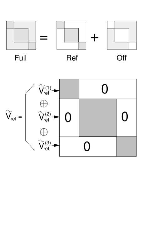
Figure 2: Full matrix $\Gamma$ expressed as a sum of the diagonal reference matrix ${\mathbf{\Gamma}}_{\rm ref}$ and the off-diagonal blocks. The matrix of reference vectors also has a block structure and is the direct sum of the row-vectors belonging to each block.

$${\mathbf{\Gamma}}_{\rm ref}={\bf U}_{\rm ref}{\bf W}_{\rm ref}\tilde{\bf V}_{\rm ref}.$$ (29)

The set of reference vectors so constructed span the same space as all of the original untreated vectors ($\tilde{\bf v}$ and $\tilde{\bf v}_{0}$ together): ${\bf V}\tilde{\bf V}={\bf V}_{\rm ref}\tilde{\bf V}_{\rm ref}$. It is convenient to define a block-label operator in terms of the reference vectors as

$${\bf P}_{op}:=\sum_{i=1}^{N_{B}}{\bf V}_{\rm ref}^{(i)}L(i)\tilde{\bf V}_{\rm ref}^{(i)},$$ (30)

where $L(i)$ is some label for block $i$(for a specific choice, see Appendix B), $N_{B}$ is the number of blocks, and ${\bf V}_{\rm ref}^{(i)}$ is the set of reference vectors belonging to block $i$. The matrix of ${\bf P}_{op}$ in the basis of the singular vectors $\bf v$ (or, analogously, ${\bf v}_{0}$, if these are needed) of the full $\mathbf{\Gamma}$ matrix is

$${\bf P}=\tilde{\bf v}{\bf P}_{op}{\bf v}=\sum_{i=1}^{N_{B}}\tilde{\bf S}_{i}{\bf S}_{i},$$ (31)

where ${\bf S}_{i}:=\sqrt{L(i)}\tilde{\bf V}_{\rm ref}^{(i)}{\bf v}$ This is equivalent to defining $\bf P$ as a product of overlap matrices expressed in terms of a matrix of the reference vectors each multiplied by the square root of their labels:

$${\bf P} = \tilde{\bf S}{\bf S},$$ (32)

$${\bf S} = \left[\sqrt{L(1)}\tilde{\bf V}_{\rm ref}^{(1)}\oplus\ldots\oplus\sqrt{L(N_{B})}\tilde{\bf V}_{\rm ref}^{(N_{B})}\right]{\bf v}.$$ (33)

See Fig. 2 for the meaning of the direct sum symbol $\oplus$. We now write $\bf S$ in terms of its singular value decomposition:

$${\bf S} = {\bf Ly}\tilde{\bf Z},$$ (34)

$$\tilde{\bf S}{\bf S} = {\bf Zy}^{2}\tilde{\bf Z}.$$ (35)

i.e. Z diagonalizes $\tilde{\bf S}{\bf S}$, the matrix of the block-label operator. The singular values of S are the square roots of the eigenvalues of the block-label operator in the basis $\bf v$. In other words, if each vector in $\tilde{\bf v}$ could be brought into coincidence with one of the reference vectors, then these vectors would have the same labels as the reference vectors. This does not, in general, occur, because the off-diagonal blocks of the $\mathbf{\Gamma}$-matrix ensure that the reference vectors cannot all be singular vectors of the full matrix; hence, the squares of the singular values of S can be used as labels of transformed vectors, $\tilde{\bf v}_{L}$:

$$\tilde{\bf v}_{L}={\tilde{\bf Z}\tilde{\bf v}}.$$ (36)

The matrix of the block-label operator in the basis ${\bf v}_{L}$ is ${\bf y}^{2}$, a diagonal matrix. This tells us that we have found a rotation (recall that $\tilde{\bf Z}{\bf Z}=\bf 1$) that associates the vectors $\tilde{\bf v}_{L}$ as closely as possible with the reference vectors. If the block-label method is to be practicable, then the values $y^{2}$ should lie close to the labels $L(i)$.

In the concrete example of Fig. 1, panel $(b)$ shows the dot products again, this time computed from vectors $\tilde{\bf v}_{0,L}$ labelled with a layer-index. The erratic behaviour has now disappeared: it is clear that one of the null vectors, (the one whose dot product is nearly zero) is now associated largely with layer 2, while the other is associated with layer 1. Note that the discontinuities coming from the arbitrary signs of the vectors still remains. This can be cured with the smoothing procedure.

III.3 The smoothing procedure

At this point, it is convenient to drop the bold-face $\bf k$, writing simply $k$ instead, since we can, without loss of generality, discuss the methodology in terms of 1-dimensional integrals only. In fact, our models employ the simple cubic lattice, where the 2-D integrals can be reduced to 1-D integrals by exploiting the symmetry in the terms containing $k_{x}$ and $k_{y}$. The first Brillouin zone is mapped onto the $k$-line in the interval $0\leq k\leq 1$. Note that $k$ is not simply the magnitude of $\bf k$, but rather a parameter which determines the value of all terms which depend on the momentum $\bf k$.

The smoothing procedure is akin to the labelling method in that untreated vectors $\tilde{\bf V}$, which we shall here refer to as target vectors, are brought into as close a coincidence as possible with the reference vectors. i.e. the target vectors are rotated to match the (fixed) reference vectors as well as possible. Here, however, the reference vectors are sets of standard vectors determined at various reference values of $k$ in the interval $0\leq k\leq 1$. As such, the reference vectors do not span exactly the same space as the set of target vectors at a neighbouring value of $k$, so a slightly different procedure must be employed. Note that in this section, the untreated vectors $\tilde{\bf V}$ (${\bf V}=({\bf v},{\bf v}_{0})$) may or may not be labelled vectors $\tilde{\bf V}_{L}$, so we shall drop the subscript $L$ for generality. If the vectors are not labelled, the method presented here must be powerful enough to cure the erratic behaviour shown in panel $(a)$ of Fig. 1, not just the sign changes shown in panel $(b)$ of the same figure. (See the dashed line in panel $(c)$ of the figure for such a case.)

We achieve the global smoothing in two stages. Prior to the integral calculation, we compute sets of well-placed reference vectors, $\{\tilde{\bf V}^{(r)}_{\rm ref};r=1,\ldots N_{r}\}$ corresponding to points in the $k$-interval. These allow us to generate by interpolation an appropriate reference vector anywhere on the $k$-interval. Then, during the calculation of the integrands in Eq. 27, we rotate the vectors $\tilde{\bf v}$ at a particular $k$ so as to match as closely as possible the interpolated reference vectors appropriate for that $k$.

To construct the sets of reference vectors, we start by obtaining the vectors $\tilde{\bf V}_{\rm ref}(k_{0})$ at some point $k_{0}$, taking these to be primary reference vectors. Moving away from $k_{0}$ a small distance (e.g. a tenth of the $k-$range), we calculate the vectors $\tilde{\bf V}(k_{1})$ at the trial point $k_{1}$ and from these, we construct a set of reference vectors $\tilde{\bf V}_{\rm ref}(k_{1})$ by a procedure designed to find the best match of $\tilde{\bf V}_{\rm ref}(k_{1})$ with $\tilde{\bf V}_{\rm ref}(k_{0})$. (An exposition of the methods to find a general rotation matching two vector spaces can be found in Appendix B.) The overlaps of corresponding vectors in the two sets are used as a criterion for accepting or rejecting the trial point. If the point is accepted, points further away are tested until either some maximum allowed distance is reached, or a point fails the test. If the first trial point is rejected, the step-size is halved to get a new test point. In this way, a set of secondary reference points can be found linking the vectors over the whole $k$-interval to the primary reference vectors. For the work reported here, sets of about 10 to 25 reference points sufficed to ensure a very large overlap (0.98, where 1.0 is “perfect”) of corresponding reference vectors at neighbouring $k$-points.

Once the sets of reference vectors are in place at the $N_{r}$ reference points $\{k_{i},i=0,1,2,\ldots,N_{r}\}$, smoothed vectors at any $k$ may be obtained in two steps: 1) a set of reference vectors at $k$ is obtained by interpolating between the vectors at the reference points $k_{l}$ and $k_{h}$ which bracket $k$: $k_{l}\leq k\leq k_{h}$. 2) The vectors $\tilde{\bf v}$ (untreated or labelled) are then rotated to be as close as possible to those in the interpolated reference set.

The computation of the interpolated reference vectors requires three steps:

1. Weights are defined for the vectors at $k_{l}$ and $k_{h}$:

   $$w_{l} = \cos^{2}{\frac{\pi}{2}\left(\frac{k-k_{l}}{k_{h}-k_{l}}\right)},$$

   $$w_{h} = 1-w_{l}.$$

2. A set of interpolated approximate reference vectors at $k$, $\widetilde{\overline{\bf V}}_{\rm ref}(k)$ is obtained as a weighted sum of the vectors at $k_{l}$ and $k_{h}$:

   $$\widetilde{\overline{\bf V}}_{\rm ref}(k)=w_{l}\tilde{\bf V}_{\rm ref}(k_{l})+w_{h}\tilde{\bf V}_{\rm ref}(k_{h}).$$ (37)

3. The approximate vectors are orthonormalized by a transformation found by diagonalizing their overlap matrix $\cal Y$:

   $${\cal Y} := \widetilde{\overline{\bf V}}_{\rm ref}\ \overline{\bf V}_{\rm ref},$$

   $${\bf\lambda} = \tilde{\bf T}{\cal Y\bf T},$$

   $${\cal Y}^{-1/2} = {\bf T\lambda}^{-1/2}\tilde{\bf T},$$

   $$\tilde{\bf V}_{\rm ref} = {\cal Y}^{-1/2}\ \widetilde{\overline{\bf V}}_{\rm ref}.$$

The overlap matrix of the transformed vectors is clearly unity:

$$\tilde{\bf V}_{\rm ref}{\bf V}_{\rm ref} = {\bf T\lambda}^{-1/2}(\tilde{\bf T}{\cal Y}{\bf T})\lambda^{-1/2}\tilde{\bf T},$$

$$= {\bf T\lambda}^{-1/2}(\lambda)\lambda^{-1/2}\tilde{\bf T},$$

$$= {\bf 1}.$$

The functional dependence of the weights chosen here ensures that the interpolated quantities are continuous and smooth at the reference points. We now have reference vectors for the non-null space and the null space (${\bf V}_{ref}=({\bf v}_{ref},{\bf v}_{0,ref})$).

The procedure for matching the untreated (or labelled) vectors $\tilde{\bf v}$ with the interpolated reference vectors $\tilde{\bf v}_{\rm ref}$ during the integrand calculation is to seek a transformation $\bf Q$ that rotates the target vectors among themselves so as to achieve the best match, just as in the labelling procedure:

$$\tilde{\bf v}_{S}={\bf Q}\tilde{\bf v}.$$ (38)

$\bf Q$ is obtained via the singular value decomposition of the overlap matrix of the reference vectors with the target vectors:

$${\cal S} := \tilde{\bf v}_{\rm ref}{\bf v},$$

$$= {\cal L}{\bf x}\tilde{\cal Z},$$

$${\bf Q} = {\cal L}\tilde{\cal Z},$$

where $\bf x$ is the diagonal matrix of singular values of the overlap matrix, which are all very close to unity by construction. $\bf Q$ is indeed a rotation because

$$\tilde{\bf Q}{\bf Q}={\cal Z}\tilde{\cal Z}=\bf 1,$$ (39)

the latter equality holding because the overlap matrix has no null space. The overlap of the transformed vectors with the reference vectors is almost the unit matrix:

$$\tilde{\bf v}_{\rm ref}{\bf v}_{S}={\cal SZ}\tilde{\cal L}={\cal L}{\bf x}\tilde{\cal Z}{\cal Z}\tilde{\cal L}={\cal L}{\bf x}\tilde{\cal L}\approx\bf 1.$$ (40)

i.e. the new vectors are as close as possible to the reference vectors. This procedure fixes the phases of the new vectors, because the transformation matrix Q is the product of the matrices $\cal L$ and $\tilde{\cal Z}$ which stem from a single SVD computation, so that the arbitrariness in the numerical determination of $\cal L$ and $\tilde{\cal Z}$ is lifted.

To summarize: the untreated vectors can be both labelled and smoothed by the transformation

$$\tilde{\bf v}_{LS}={\bf Q}\tilde{v}_{L}={\cal L}\tilde{\cal Z}\tilde{\bf Z}\tilde{\bf v}.$$ (41)

In our concrete example, the effect of the smoothing operation is seen in panel $(c)$ of Fig. 1. The solid lines are the result of applying the smoothing to the labelled vectors in panel $(b)$: $\tilde{\bf v}_{0,SL}={\cal L}\tilde{\cal Z}\tilde{\bf Z}\tilde{\bf v}_{0}$, where $\tilde{\bf v}_{0}$ are the untreated vectors labelled only by the singular values $0$. The dashed lines result from smoothing the untreated vectors in panel $(a)$: $\tilde{\bf v}_{0,S}={\cal L}\tilde{\cal Z}\tilde{\bf v}_{0}$.

In our example, we have not attempted to calibrate the primary vectors in any way, but this could be done if desired; however, this would still be a very crude way of labelling the vectors. A more important function of the primary vector is to ensure that all points in the region of a given point are related to one another. $k$ is not the only parameter determining the elements of the $\mathbf{\Gamma}$-matrix; the expectation values of the spin operators are others. In particular, if the derivatives of some quantity with respect to any of these parameters is needed, then it is a good idea to retain some standard vector with which to calibrate the primary vectors for all points in the neighbourhood of some given point.

IV Heisenberg Hamiltonian with exchange anisotropy

IV.1 Algebraic formulation

In order to illustrate the labelling and smoothing procedures described here, we consider the model of referenceFK02 , a Heisenberg Hamiltonian with an exchange anisotropy for thin ferromagnetic films. In contrast to the work in referenceFK03 , the projector onto the null space here depends on the momentum. To show the importance of the labelling procedure, we need to extend the model of reference FK03 to multilayer thin films.

In what follows, a composite subscript of the type $k_{\kappa}$ refers to the site $k$ in layer $\kappa$. We shall consider only nearest neighbour interactions in a simple cubic lattice structure. The Hamiltonian is characterized by an exchange interaction with strength ($J_{k_{\kappa}l_{\lambda}}>0$) between nearest neighbour lattice sites, a uniaxial exchange anisotropy in the z-direction with strength ($D_{k_{\kappa}l_{\lambda}}>0$), and an external magnetic field ${\bf B}=(B^{x},0,B^{z})$ confined to the reorientation plane of the magnetization:

$${\cal H}= - \frac{1}{2}\sum_{<k_{\kappa}l_{\lambda}>}J_{k_{\kappa}l_{\lambda}}(S_{k_{\kappa}}^{-}S_{l_{\lambda}}^{+}+S_{k_{\kappa}}^{z}S_{l_{\lambda}}^{z})$$ (42)

$$- \frac{1}{2}\sum_{<k_{\kappa}l_{\lambda}>}D_{k_{\kappa}l_{\lambda}}S_{k_{\kappa}}^{z}S_{l_{\lambda}}^{z}$$

$$- \sum_{k}\Big{(}B^{x}\frac{1}{2}(S_{k_{\kappa}}^{+}+S_{k_{\kappa}}^{-})+B^{z}S_{k_{\kappa}}^{z}\Big{)}.$$

Here the notation $S_{k_{\kappa}}^{\pm}=S_{k_{\kappa}}^{x}\pm iS_{k_{\kappa}}^{y}$ is introduced, where $k_{\kappa}$ and $l_{\lambda}$ are lattice site indices and $<k_{\kappa}l_{\lambda}>$ indicates summation over nearest neighbours only. To fully describe magnetization in the $xz$-plane for arbitrary spin $S$, Green’s functions of the following type are required:

$$G_{r_{\rho},s_{\sigma}}^{\alpha,mn}=\ll S_{r_{\rho}}^{\alpha};(S_{s_{\sigma}}^{z})^{m}(S_{s_{\sigma}}^{-})^{n}\gg,$$ (43)

where $\alpha$ is one of $\{+,-,z\}$ and $m$ and $n$ are integers which are determined by the spin $S$. The equation of motion for this Green’s function is

$$\omega G_{r_{\rho},s_{\sigma}}^{\alpha,mn} = A_{r_{\rho},s_{\sigma}}^{\alpha,mn}+\ll\left[S_{r_{\rho}}^{\alpha},{\cal H}\right]_{-};(S_{s_{\sigma}}^{z})^{m}(S_{s_{\sigma}}^{-})^{n}\gg,$$

$$A_{r_{\rho},s_{\sigma}}^{\alpha,mn} = \left\langle\left[S_{r_{\rho}}^{\alpha},(S_{s_{\sigma}}^{z})^{m}(S_{s_{\sigma}}^{-})^{n}\right]_{-}\right\rangle.$$ (44)

The generalized Tyablikov decoupling approximationTya59 is now applied to each Green’s function on the rhs of the equation of motion, e.g.

$$\ll S_{r_{\rho}}^{\alpha}S_{t_{\tau}}^{\beta};\ldots\gg\approx\langle S_{r_{\rho}}^{\alpha}\rangle\ G_{t_{\tau},s_{\sigma}}^{\beta,mn}+\langle S_{t_{\tau}}^{\beta}\rangle\ G_{r_{\rho},s_{\sigma}}^{\alpha,mn}.$$ (45)

Elimination of the site indices by means of a Fourier transformation to momentum space results in the matrix form of the equations of motion shown in Eq. 1. The components in the Green’s function vector have the superscripts $\alpha$ and $mn$ and two subscript layer-indices and depend on energy and momentum: $G_{\rho\sigma}^{\alpha,mn}(\omega,\bf k)$.

IV.1.1 The 3-layer model

We now specialize the exposition to the 3-layer film, since it is the smallest non-trivial example from which the extension to larger films is obvious. For this case, Eq. 1 has the following structure:

$$\left[\omega{\bf 1}-\left(\begin{array}[]{ccccccccc}\Gamma_{11}&\Gamma_{12}&0&0&0&0&0&0&0\\ \Gamma_{21}&\Gamma_{22}&\Gamma_{23}&0&0&0&0&0&0\\ 0&\Gamma_{32}&\Gamma_{33}&0&0&0&0&0&0\\ 0&0&0&\Gamma_{11}&\Gamma_{12}&0&0&0&0\\ 0&0&0&\Gamma_{21}&\Gamma_{22}&\Gamma_{23}&0&0&0\\ 0&0&0&0&\Gamma_{32}&\Gamma_{33}&0&0&0\\ 0&0&0&0&0&0&\Gamma_{11}&\Gamma_{12}&0\\ 0&0&0&0&0&0&\Gamma_{21}&\Gamma_{22}&\Gamma_{23}\\ 0&0&0&0&0&0&0&\Gamma_{32}&\Gamma_{33}\end{array}\right)\right]$$ (55)

$${\Large\times}\left(\begin{array}[]{c}G_{11}\\ G_{21}\\ G_{31}\\ G_{12}\\ G_{22}\\ G_{32}\\ G_{13}\\ G_{23}\\ G_{33}\end{array}\right)=\left(\begin{array}[]{c}A_{11}\\ 0\\ 0\\ 0\\ A_{22}\\ 0\\ 0\\ 0\\ A_{33}\end{array}\right).\rule{51.21504pt}{0.0pt} \ .$$ (74)

Each of the entries in the $9\times 9$ matrix ${\mathbf{\Gamma}}$ is in fact a $3\times 3$ matrix corresponding to a Green’s function vector with the same $mn$ values and layer subscripts but with superscripts $\alpha=\{+,-,z\}$ characterizing the vector components. Using $i$ as a layer-index, the diagonal matrix ${\mathbf{\Gamma}_{ii}}$ is

$${{\mathbf{\Gamma}}_{ii}}=\left(\begin{array}[]{@{\hspace*{3mm}}c@{\hspace*{5mm}}c@{\hspace*{5mm}}c@{\hspace*{3mm}}}\hskip 8.53581pt\lx@intercol\hfil\;\;\;H^{z}_{i}\hfil\hskip 14.22636pt&0\hfil\hskip 14.22636pt&-H^{x}_{i}\hfil\hskip 8.53581pt\\ \hskip 8.53581pt\lx@intercol\hfil 0\hfil\hskip 14.22636pt&-H^{z}_{i}\hfil\hskip 14.22636pt&\;\;\;H^{x}_{i}\hfil\hskip 8.53581pt\\ \hskip 8.53581pt\lx@intercol\hfil-\frac{1}{2}\tilde{H}^{x}_{i}\hfil\hskip 14.22636pt&\;\frac{1}{2}\tilde{H}^{x}_{i}\hfil\hskip 14.22636pt&0\hfil\hskip 8.53581pt\end{array}\right)\ .$$ (75)

where

$$H^{z}_{i} = Z_{i}+\langle S_{i}^{z}\rangle J_{ii}(q-\gamma_{\bf k})\ ,$$

$$Z_{i} = B^{z}+D_{ii}q\langle S^{z}_{i}\rangle+(J_{i,i+1}+D_{i,i+1})\langle S_{i+1}^{z}\rangle$$ (76)

$$+(J_{i,i-1}+D_{i,i-1})\langle S_{i-1}^{z}\rangle\ ,$$

$$\tilde{H}^{x}_{i} = B^{x}+\langle S_{i}^{x}\rangle J_{ii}(q-\gamma_{\bf k})+J_{i,i+1}\langle S_{i+1}^{x}\rangle+J_{i,i-1}\langle S_{i-1}^{x}\rangle\ ,$$

$$H^{x}_{i} = \tilde{H}^{x}_{i}-\langle S_{i}^{x}\rangle D_{ii}\gamma_{\bf k}\ .$$

For a square lattice and a lattice constant taken to be unity, $\gamma_{\bf k}=2(\cos k_{x}+\cos k_{y})$, and $q=4$ is the number of intra-layer nearest neighbours. The off-diagonal sub-matrices ${\bf\Gamma}_{ij}$ for $j=i\pm 1$ are of the form

$${\bf\Gamma}_{ij}=\left(\begin{array}[]{ccc}-J_{ij}\langle S_{i}^{z}\rangle&0&\;\;\;(J_{ij}+D_{ij})\langle S_{i}^{x}\rangle\\ 0&\;\;J_{ij}\langle S_{i}^{z}\rangle&-(J_{ij}+D_{ij})\langle S_{i}^{x}\rangle\\ \frac{1}{2}J_{ij}\langle S_{i}^{x}\rangle&-\frac{1}{2}J_{ij}\langle S_{i}^{x}\rangle&0\end{array}\right)\;.$$ (77)

Unlike the elements of the $\mathbf{\Gamma}$-matrix, the components of the vectors $\bf C$ and $\bf A$ are dependent on the values of $m$ and $n$. For spin $S=1$, the values of $(m,n)$ required are $(0,1)$ and $(1,1)$. The values of the diagonal correlations $C_{ii}$ and $A_{ii}$ for each value of $\alpha$ are shown in Table 1. The layer index $i$ has been omitted for brevity.

Table 1: Diagonal correlations and inhomogeneities for spin $S=1$.

	$\alpha$	$mn=(0,1)$	$mn=(1,1)$
	+	$\langle 2S^{z}\rangle$	$-2-\langle S^{z}\rangle+3\langle S^{z}S^{z}\rangle$
$\bf A$	-	$0$	$\langle S^{x}S^{x}\rangle$
	$z$	$-\langle S^{x}\rangle$	$-\langle S^{z}S^{x}\rangle$
	+	$2-\langle S^{z}\rangle-\langle S^{z}S^{z}\rangle$	$\langle S^{z}\rangle-\langle S^{z}S^{z}\rangle$
$\bf C$	-	$\langle S^{x}S^{x}\rangle$	$\langle S^{z}S^{x}S^{x}\rangle$
	$z$	$\langle S^{x}\rangle+\langle S^{z}S^{x}\rangle$	$\langle S^{z}S^{x}\rangle+\langle S^{z}S^{z}S^{x}\rangle$

The block-diagonal structure of the matrix in Eq. 74 allows us to write Eq. 74 in terms of Green’s functions and inhomogeneities labelled by a single layer index $i$. Define singly-indexed Green’s function vectors (here $3\times 3=9$ components),their corresponding correlations, and inhomogeneities for $\{i=1,2,3\}$.

$$\begin{array}[]{ccc}G_{i}=\left(\begin{array}[]{c}G_{1i}\\ G_{2i}\\ G_{3i}\end{array}\right),&C_{i}({\bf k})=\left(\begin{array}[]{c}C_{1i}\\ C_{2i}\\ C_{3i}\end{array}\right),&A_{i}=\left(\begin{array}[]{c}A_{1i}\delta_{1i}\\ A_{2i}\delta_{2i}\\ A_{3i}\delta_{3i}\end{array}\right).\end{array}$$

The $(9\times 9)$ matrices are independent of an index:

$$\Gamma=\left(\begin{array}[]{ccc}\Gamma_{11}&\Gamma_{12}&0\\ \Gamma_{21}&\Gamma_{22}&\Gamma_{23}\\ 0&\Gamma_{32}&\Gamma_{33}\end{array}\right).$$ (78)

The big equations can now be replaced by 3 smaller equations of motion and correlation equations $i=1,2,3$:

$$\left(\omega{\bf 1}-\Gamma\right)G_{i} = A_{i},$$ (79)

$$({\bf 1}-{\bf R}^{0}{\bf L}^{0})C_{i}({\bf k}) = {\bf R}^{1}{\cal E}^{1}{\bf L}^{1}{A_{i}}.$$ (80)

Applying the SVD to $\Gamma$ yields six vectors $\tilde{\bf v}$ in the non-null space (each layer contributes one null vector). The corresponding six correlations $\bf c$ are obtained by multiplying the last equation by $\tilde{\bf v}$ and inserting ${\bf v}\tilde{\bf v}+{\bf v}_{0}\tilde{\bf v}_{0}=\bf 1$:

$$\tilde{\bf v}({\bf 1}-{\bf R}^{0}{\bf L}^{0})C_{i}({\bf k})={\bf R}^{1}{\cal E}^{1}{\bf L}^{1}({\bf v}\tilde{\bf v}+{\bf v}_{0}\tilde{\bf v}_{0})A_{i}.$$ (81)

Use of $\tilde{\bf v}{\bf R}^{0}={\bf 0}$, ${\bf L}^{1}{\bf v}_{0}={\bf 0}$ (see Appendix A), ${\bf r}=\tilde{\bf v}{\bf R}^{1}$, and ${\bf l}={\bf L}^{1}{\bf v}$ leads to

$$\tilde{\bf v}C_{i}({\bf k})={\bf r}{\cal E}^{1}{\bf l}\tilde{\bf v}A_{i},$$ (82)

which, after integration over $\bf k$ corresponds to Eq. 27.

IV.1.2 Analytical algebraic results for the monolayer

We now investigate in detail the monolayer for spin $S=1$, for which many results can be obtained analytically and reveal features which are pertinent to the structures found for the multilayers .

The monolayer model leads to an equation of motion with the single diagonal block ${\mathbf{\Gamma}}_{11}$ and the vectors ${\bf G}_{11}$, ${\bf C}_{11}$, and ${\bf A}_{11}$. For the remainder of this section, we shall drop the subscripts $11$. The eigenvalues of $\mathbf{\Gamma}$ are $\{0,\epsilon_{k},-\epsilon_{k}\}$, where $\epsilon_{k}=\sqrt{H^{z}H^{z}+H^{x}\tilde{H^{x}}}$. The matrices of eigenvalues and eigenvectors of $\mathbf{\Gamma}$ are then

$${\bf L}{\mathbf{\Gamma}}{\bf R} = \Omega=\left(\begin{array}[]{ccc}0&0&0\\ 0&\epsilon_{k}&0\\ 0&0&-\epsilon_{k}\end{array}\right),$$ (86)

$${\bf R} = \left(\begin{array}[]{ccc}\frac{H^{x}}{H^{z}}&\frac{-(\epsilon_{k}+H^{z})}{\tilde{H}^{x}}&\frac{(\epsilon_{k}-H^{z})}{\tilde{H}^{x}}\\ \frac{H^{x}}{H^{z}}&\frac{(\epsilon_{k}-H^{z})}{\tilde{H}^{x}}&\frac{-(\epsilon_{k}+H^{z})}{\tilde{H}^{x}}\\ 1&1&1\end{array}\right),$$ (90)

$${\bf L} = \frac{1}{4\epsilon_{k}^{2}}\left(\begin{array}[]{ccc}2\tilde{H}^{x}H^{z}&2\tilde{H}^{x}H^{z}&4H^{z}H^{z}\\ -(\epsilon_{k}+H^{z})\tilde{H}^{x}&(\epsilon_{k}-H^{z})\tilde{H}^{x}&2H^{x}\tilde{H}^{x}\\ (\epsilon_{k}-H^{z})\tilde{H}^{x}&-(\epsilon_{k}+H^{z})\tilde{H}^{x}&2H^{x}\tilde{H}^{x}\end{array}\right).$$ (94)

Taking the first row of $\bf L$ from Eq. 90 and the inhomogeneity vectors for $mn=\{0,1\}$ from Table 1, we find from the regularity condition ${\bf L}^{0}{\bf A}={\bf 0}$,

$$\frac{\tilde{H}^{x}}{H^{z}}=\frac{\langle S^{x}\rangle}{\langle S^{z}\rangle}.$$ (95)

This implies that the ratio on the lhs is not dependent upon the momentum. This can also be seen directly from the definitions in Eq. IV.1.1:

$$\frac{\langle S^{x}\rangle}{\langle S^{z}\rangle}=\frac{B^{x}}{B^{z}+Dq\langle S^{z}\rangle}.$$ (96)

From the same definitions it is clear that the ratio $\frac{H^{x}}{H^{z}}$ does depend upon momentum because $H^{x}$ differs from $\tilde{H}^{x}$ by a momentum-dependent term; hence the projector ${\bf R}^{0}{\bf L}^{0}$ onto the null space is momentum dependent.

The singular vectors in $\bf U$ and $\bf V$ (see Eq. 20) may be obtained as the eigenvectors of the symmetric matrices $\mathbf{\Gamma}\tilde{\mathbf{\Gamma}}$ and $\tilde{\mathbf{\Gamma}}\mathbf{\Gamma}$, respectively. The singular values in $\bf W$ are the square roots of the eigenvalues of these matrices.

$$\bf W = \left(\begin{array}[]{ccc}W_{11}&0&0\\ 0&W_{22}&0\\ 0&0&0\end{array}\right),$$ (100)

$$W_{11} = \sqrt{H^{z}H^{z}+2H^{x}H^{x}},$$ (101)

$$W_{22} = \sqrt{H^{z}H^{z}+\frac{1}{2}\tilde{H}^{x}\tilde{H}^{x}},$$ (102)

$$\bf U = \left(\begin{array}[]{cc|c}-\frac{1}{\sqrt{2}}&\frac{-H^{z}}{\sqrt{2}W_{22}}&\frac{\tilde{H}^{x}}{2W_{22}}\\[5.69054pt] \frac{1}{\sqrt{2}}&\frac{-H^{z}}{\sqrt{2}W_{22}}&\frac{\tilde{H}^{x}}{2W_{22}}\\[5.69054pt] 0&\frac{\tilde{H}^{x}}{\sqrt{2}W_{22}}&\frac{H^{z}}{W_{22}}\end{array}\right),$$ (106)

$$\tilde{\bf V} = \left(\begin{array}[]{ccc}\frac{-H^{z}}{\sqrt{2}W_{11}}&\frac{-H^{z}}{\sqrt{2}W_{11}}&\frac{2H^{x}}{\sqrt{2}W_{11}}\\[5.69054pt] \frac{-1}{\sqrt{2}}&\frac{1}{\sqrt{2}}&0\\[5.69054pt] \hline\cr&&\\[-11.38109pt] \frac{H^{x}}{W_{11}}&\frac{H^{x}}{W_{11}}&\frac{H^{z}}{W_{11}}\end{array}\right).$$ (111)

The matrix $\bf U$ has been blocked into $\bf u$ and ${\bf u}_{0}$ by the vertical line and $\tilde{\bf V}$ into $\tilde{\bf v}$ and $\tilde{\bf v}_{0}$ by the horizontal line. We see here explicitly (by factoring out $H^{z}$ and applying the regularity condition) that the vector ${\bf L}_{0}$, the first row-vector in the matrix ${\bf L}$ in Eq. 90, is proportional to the vector ${\bf u}_{0}$ and is independent of momentum. In fact, the vectors in $\bf u$ are also independent of momentum. Similarly, ${\bf R}_{0}$ is proportional to ${\bf v}_{0}$, but does depend upon momentum. As the momentum varies, $\tilde{\bf v}_{0}$ also varies but remains in the plane containing the $G^{z}$-axis and the line bisecting the axes $G^{+}$ and $G^{-}$. This implies that one of the vectors in the non-null space can be chosen to be perpendicular to this plane and therefore must be independent of momentum. This is the second row-vector in $\tilde{\bf V}$ in Eq. 111. The first row-vector in $\tilde{\bf V}$ is also dependent upon momentum and lies in the same plane as the null vector.

From these considerations, it is clear that, for the monolayer, only the second row-vector of $\tilde{\bf V}$ in Eq. 111 is momentum-independent; hence, only the second row from Eq. 82 (here specialized to the monolayer) can be used in the consistency equations. For spin $S=1$, there are two expectation values which act as the variables which must be iterated to self-consistency in Eq. 27, $\langle S^{z}\rangle$ and $\langle S^{z}S^{z}\rangle$. Since only one row of Eq. 82 can be used, it is necessary to use this equation twice, each time with different values of $mn$ (see Table 1). The other correlations in Table 1 can be expressed in terms of $\langle S^{z}\rangle$ and $\langle S^{z}S^{z}\rangle$ via the regularity condition ${\bf L}^{0}{\bf A}^{mn}={\bf 0}$, for $m+n\leq 2S+1$ (for details see FJKE00 ).

In the multilayer case, each layer supplies an extra row in Eq. 82 which can be used as a consistency equation, so that there are just enough equations to solve for the expectation values $\langle S^{z}_{i}\rangle$ and $\langle S^{z}_{i}S^{z}_{i}\rangle$ for each layer $i$.

IV.1.3 Algebraic properties of the multilayers

While it is not practicable to perform the singular value decomposition algebraically for the multilayer films, it is nevertheless possible to deduce some properties of the singular vectors by examining the results for the monolayer and combining these with the structure of the $3\times 3$ blocks of the matrix $\mathbf{\Gamma}$ in Eq. 74.

We start with the structure of the null vectors of the matrix $\mathbf{\Gamma}$ from Eq. 78 in a film of $N$ layers. We may write a null row-vector in terms of the three components for each layer as

$$\tilde{\bf v}_{0}=(\tilde{v}_{0}^{(1)},\ldots,\tilde{v}_{0}^{(N)})$$ (112)

There are $N$ null vectors each with $3N$ components. We see from Eq. 111 that the components $\tilde{v}_{0}^{(i)}$ of the null vector for the $i$th layer considered in isolation have the form $(a_{i},a_{i},b_{i})$. But this must also hold for each of the null vectors in Eq. 112. To see this, consider the $\mathbf{\Gamma}$-matrix of Eq. 78 extended to $N$ layers acting on a single null vector:

$${\mathbf{\Gamma}}{\bf v}_{0}=\bf 0$$ (113)

This gives $3N$ equations for the components of ${\bf v}_{0}$, 3 for each layer. Denote the components belonging to layer $i$ as $(x_{i},y_{i},z_{i})$ Now the structure of the $3\times 3$ blocks in $\mathbf{\Gamma}$ is such that the first equations for each layer (i.e. equations $1,4,7,\ldots$) involve only the components $x_{i}$ and $z_{i}$ for all $i$; i.e. the $N$ equations suffice to determine the $N$ ratios $x_{i}/z_{i}$. The second equations for each layer (i.e. $2,5,8,\ldots$) involve only $y_{i}$ and $z_{i}$ and they are exactly the same as the first equations for each layer. The components $x_{i}$ are therefore the same as the $y_{i}$. But this implies, from the structure of the blocks in $\mathbf{\Gamma}$, that the third equations for each layer are then automatically satisfied. The values of the $x_{i}$, $y_{i}$, and $z_{i}$ are then obtained from normalization. This means that each null vector, although perhaps dependent upon the momentum, must lie in the hyperplane in which the components belonging to layer $i$ have the form $(a_{i},a_{i},b_{i})$. This, in turn, means that the hyperplane in which all layer components have the form $(c_{i},-c_{i},0)$ must lie in the non-null space and be independent of momentum, since each vector of this form is obviously orthogonal to each null vector.

Consider now special vectors of this form for which the components for layer $i$ are $(c_{i},-c_{i},0)$ but all other components are zero, i.e. $N$ of the $3N$ reference vectors of Eq. 29, $\tilde{\bf V}_{\rm ref}$. Clearly, these vectors are also in the non-null space and are orthogonal to each other. This is the reason why the labelling procedure picks out these particular reference vectors as being identical with some of the vectors $\tilde{\bf v}$. Of course, the rest of the vectors $\tilde{\bf v}$ are not in general identical to any of the remaining $2N$ reference vectors, because the null vectors do not in general have a layer-structure, implying that each of the remaining reference vectors lies partially in the null space. All of these features are fully verified by the numerical calculations of the next section.

In summary, we see that in the $N$-layer film, there are only $N$ components of the vector $\bf c$ from Eq. 82 (for a given value of $mn$) which are independent of momentum and also possess a layer-structure. The numerical labelling procedure is capable of delivering these vectors. This bit of serendipity is essential to the success of the entire method, since we only know how to determine the diagonal correlations, $C_{ii}$, from the expectation values; hence, we require that the dot product of our vector with $C_{i}({\bf k})$ only involve the component $C_{ii}$. This is ensured by the aforementioned property of those (labelled) vectors in $\tilde{\bf v}$ which are independent of momentum. In contrast, the momentum-dependent vectors in $\tilde{\bf v}$ do not share this property and therefore cannot be used in solving the consistency equations (27).

IV.2 Numerical results

We conclude our exposition with a few illustrative numerical calculations for the $S=1$ Heisenberg Hamiltonian model with exchange anisotropy of Eq. 42. The exchange energy is $J=100$, the exchange anisotropy is $D=0.7$, and the field in the $z$-direction is zero. We show, as representative examples, some results of calculations for 1-, 3-, and 7-layer films.

First, the labelled and smoothed row-vectors $\tilde{\bf V}$ (${\bf V}=({\bf v},{\bf v_{0}})$) are shown in Table 2 for a 3-layer film with $B^{x}=0.1,B^{z}=0$ at $T=107$, which is very near the reorientation temperature of the magnetization, $T_{R}$. Displayed are the six vectors in the non-null space, $\tilde{\bf v}$, and the three null vectors, $\tilde{\bf v}_{0}$, at $k=0.0100113$.

Table 2: Row-vectors $\tilde{\bf V}$ at $k=0.0100113$ for the 3-layer film.

Layer		1			2			3
$\alpha$	+	-	z	+	-	z	+	-	z
	0.71	-0.71	0	0	0	0	0	0	0
	0.46	0.46	-0.76	0.03	0.03	0.04	0.01	0.01	0.02
$\tilde{\bf v}$	0	0	0	0.71	-0.71	0	0	0	0
	0.02	0.02	0.02	0.47	0.47	-0.74	0.02	0.02	0.02
	0	0	0	0	0	0	0.71	-0.71	0
	0.01	0.01	0.02	0.03	0.03	0.04	0.46	0.46	-0.76
	0.54	0.54	0.65	-0.02	-0.02	0.025	-0.01	-0.01	0.02
$\tilde{\bf v}_{0}$	0.02	0.02	-0.04	-0.53	-0.53	-0.67	0.02	0.02	-0.04
	0.01	0.01	-0.02	0.02	0.02	-0.03	-0.54	-0.54	-0.65

Figure 3: One component of a momentum-dependent vector $\tilde{\bf v}$ for the 3-layer film near the Reorientation temperature of the magnetization ($T=107$) at the reference points $k_{i}$.

Vectors 1,3, and 5 are independent of momentum and have a layer-structure: i.e. they may be identified with layers 1,2, and 3, respectively. In contrast to this, vectors 2, 4, and 6 have contributions from each layer. Nevertheless, each of these vectors can be labelled by the layers 1,2, and 3, respectively, because the contributions from those layers are by far the greatest in each respective vector. The null-vectors are similar to vectors 2, 4, and 6: they vary with $k$, have no layer-structure, but may be labelled with a layer index.

A component of one of the vectors $\tilde{\bf v}$ is shown in Fig. 3 at the reference points $k_{i}$ for one of the momentum-dependent vectors for the 3-layer film at a temperature $T=107$ near the reorientation temperature of the magnetization. Since there is rapid variation near $k=0$, the number of reference points there is denser than at larger $k$. At smaller temperatures, this behaviour is not as extreme.

Fig. 4 displays the most rapidly varying component of one of the momentum-dependent labelled vectors $\tilde{\bf v}$ in the non-null space as a function of the momentum $k$ over the first tenth of the $k$-range for the monolayer at $T=0$; the curves remain roughly constant over the rest of the range. For increasing magnetic field in the $x$-direction, $B^{x_{i}}$, the curves become steeper near $k=0$, becoming nearly L-shaped for the largest field value (corresponding to $\langle S^{z}\rangle\rightarrow 0$). A greater density of reference vectors (positions are indicated by the full circles) is needed in this range. Nevertheless, the smoothing procedure is able to deliver acceptable vectors even under these extreme conditions. Note that $all$ the vectors $\tilde{\bf v}$ in the non-null space are needed accurately, not just those that are independent of momentum, because they are employed in reducing the size of the $\mathbf{\Gamma}$-matrix by the transformation in Eqns. 21 to 24.

Figure 4: A single component of one of the vectors in $\tilde{\bf v}$ for the monolayer as a function of momentum $k$ for increasing values of magnetic field $B^{x}$: $B^{x_{0}}\approx 0<B^{x_{1}}\ldots<B^{x_{3}}\approx 1.3$. The circles indicate the position of the reference vectors.

We now present the magnetizations calculated by solving Eq. 27 self-consistently as a function of magnetic field and temperature. Fig. 5 shows the magnetization $\langle S^{z}\rangle$ (beginning at 1 at $B^{x}=0$), the magnetization $\langle S^{x}\rangle$ increasing linearly from 0, the reorientation angle of the magnetization, $\Theta$, and the absolute value of the total magnetization for a spin $S=1$ Heisenberg monolayer as functions of the applied magnetic field in the $x$-direction, $B^{x}$ at temperature $T=0$. (Results at other temperatures are similar.)

Figure 5: Magnetization components $\langle S^{z}\rangle$ ($=1$ at $B^{x}=0$) and $\langle S^{x}\rangle$ (solid lines), the reorientation angle of the magnetization, $\Theta=(\arctan{\frac{\langle S^{x}\rangle}{\langle S^{z}\rangle}})/\frac{\pi}{2}$ (dashed line), and the absolute value of the total magnetization (dash-dot chain) for a spin S=1 Heisenberg monolayer as functions of the applied magnetic field in the $x$-direction, $B^{x}$, at $T=0$.

Magnetization components as a function of temperature are shown for the 3-layer film in Fig. 6. Magnetizations for layers 1 and 3 are identical as required by symmetry. Because the magnetic field component ${B}^{x}$ is so small, the 3 components in the $x$-direction cannot be distinguished from one another on the scale of the diagram.

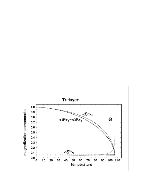
Figure 6: Magnetization components in different layers $\langle S^{z}\rangle_{i}$ and $\langle S^{x}\rangle_{i}$ (solid lines) and the reorientation angle of the magnetization (dashed line), for a spin $S=1$ Heisenberg trilayer as functions of the temperature, $T$, at $B^{x}=0.1$

Fig. 7 demonstrates that it is also no problem to calculate the reorientation of the magnetization for a film consisting of $7$ layers. Films with spin $S>1$ can also be treated. In fact, all of our previous work on this modelFK02 can be reproduced with the present method, so there is no need to present more examples here.

Figure 7: Magnetization components in different layers $\langle S^{z}\rangle_{i}$ and $\langle S^{x}\rangle_{i}$ (solid lines) and the reorientation angle of the magnetization (dashed line), for a spin $S=1$ Heisenberg $7$-layer film as functions of the temperature, $T$, at $B^{x}=0.1$

V A more efficient algorithm

In this section, we shall establish the connection between the method developed here and the one we used in our previous work on ferromagnetic Heisenberg films with exchange anisotropyFK02 . To do this, the working equations are cast in a slightly different form that in some cases allows one to dispense with the smoothing procedure. This suggests that the new method serves not only as a tool to find appropriate consistency equations but also as a means of designing an efficient algorithm for solution.

Our method has so far employed the matrix of singular vectors $\tilde{\bf v}$ to transform the correlations in momentum space (${\bf c}=\tilde{\bf v}{\bf C_{k}}$) so that ${\bf c}$ can be expressed via Eq. 26 in terms of quantities referring only to the non-null space of the matrix $\mathbf{\Gamma}$. Via the labelling procedure, the row-vectors $\tilde{\bf v}$ were then transformed so that a subset of them were independent of momentum; hence, the result in Eq. 28 could be exploited in the consistency equations Eq. 27. Let us now multiply the rhs of Eq. 26 by the unit matrix $\tilde{\bf v}{\bf v}$:

$$\tilde{\bf v}{\bf C}_{\bf k}=\tilde{\bf v}({\bf v}{\bf r}{\cal E}^{1}{\bf l\tilde{\bf v}A}).$$ (114)

Consider now the consistency equation obtained from the momentum-independent vector $\tilde{\bf v}_{j}$, which we take as the second row-vector $\tilde{\bf V}$ in Eq. 111 (refer also to Eq. 28):

$$\tilde{\bf v}_{j}\int d{\bf k}\ {\bf C}_{\bf k}=\tilde{\bf v}_{j}{\bf C}=\int d{\bf k}\ \tilde{\bf v}_{j}({\bf v}{\bf r}{\cal E}^{1}{\bf l\tilde{\bf v}A}).$$ (115)

There is one such equation for each layer. Taken together, these equations succinctly describe the method of solution in reference FK02 , where, for each layer, a difference of correlations (the lhs) was related to the difference between the first and second integrated components of the rhs of the equation in round brackets. The idea to build this difference of components came from the empirical observation (by taking linear combinations of the equations of the standard procedure in the full space) that such difference terms make no contribution to the momentum-dependent term ${\bf R}^{0}{\bf L}^{0}$, thus eliminating the latter from the consistency equations. Here (Eq. 115), taking the difference is effected via multiplication by the vectors $\tilde{\bf v}_{j}$ found systematically from the SVD coupled with the labelling procedure, thus replacing intuition with a systematic approach.

The advantage of this way of solving the equations is that in this case there is no need to apply the smoothing procedure at each value of $\bf k$, since the singular vectors $\bf v$ and $\tilde{\bf v}$ now both occur in the product in the integrand; i.e. an arbitrary sign arising from $\tilde{\bf v}$ is offset by that from $\bf v$. We emphasize that smoothing would still be needed if there were degeneracies in the non-zero singular values, which was not the case in our previous work. Also, the labelling and smoothing procedures are required to find the appropriate $\tilde{\bf v}_{j}$ in the diagnostic phase of the work.

This suggests that the procedure in this paper can be used as a tool to find appropriate vectors $\tilde{\bf v}_{LS}$ via the labelling and smoothing procedures and then, once the vectors have been found, to design a more efficient numerical procedure. We note here that the momentum-independent vectors for the exchange anisotropy model are particularly simple, being in fact just numbers. This need not always be the case: in general, these vectors will depend on the magnetizations and will vary as one moves through solution space (e.g. magnetizations as a function of temperature). In this case, a method of the type suggested above would require that the diagnostic tool be built into the numerical algorithm in order to find the appropriate vectors at each point in space.

VI Discussion

The main thrust of this paper is to demonstrate that the SVD is a very powerful tool for solving the problems which arise when the equations of motion matrix $\mathbf{\Gamma}$ has zero eigenvalues. In particular, the singular vectors in the non-null space, $\tilde{\bf v}$, are used to reduce the size of the matrix that needs to be diagonalized and, at the same time, increase the numerical stability by eliminating the zero eigenvalues and the degeneracy associated with them, a fact of considerable practical importance, especially when some of the non-zero eigenvalues lie close to zero. In addition, the suitably labelled and smoothed singular vectors $\tilde{\bf v}_{LS}$ serve to transform the consistency equations so as to deliver the correlation functions in coordinate space required for the solution of these equations.

The method outlined here can be viewed as a recipe for direct numerical calculation . The recipe is quite simple:

1. At the current point in solution space, generate a sufficient number of reference vectors $\tilde{\bf V}_{\rm ref}(k_{i})$ at suitably chosen knots $k_{i}$.
   

2. At each desired value of $k$,

   1. Obtain the untreated singular vectors $\tilde{\bf v}$ in the non-null space from the SVD of the $\mathbf{\Gamma}$-matrix.
      

   2. If necessary, find labelled vectors from these: $\tilde{\bf v}_{L}=\tilde{\bf Z}\tilde{\bf v}$. If no labelling is desired, set $\tilde{\bf Z}=1$ at this point.
      

   3. Find the set of smoothed reference vectors appropriate to $k$ and carry out the smoothing transformation: $\tilde{\bf v}_{LS}={\cal L}\tilde{\cal Z}\tilde{\bf Z}\tilde{\bf v}$.
      

   4. Use the smoothed vectors to reduce the $\mathbf{\Gamma}$-matrix by eliminating the null space. Diagonalize the reduced matrix to get the eigenvalues and eigenvectors: $\bf l{\mathbf{\gamma}}\bf r={\mathbf{\omega}}^{1}$
      

   5. Select the appropriate (i.e. properly labelled momentum-independent) vectors $\tilde{\bf v}$ to generate the set of consistency integrands of Eq. 27: ${\bf r}{\cal E}{\bf l}\tilde{\bf v}{\bf A}-\tilde{\bf v}{\bf C}_{\bf k}$
      

3. Finally, solve the consistency equations Eq. 27 (e.g. with the method described in FKS02 ).

This recipe cannot be so general as to apply to any problem, for the labelling is dictated by the properties of the $\mathbf{\Gamma}$-matrix, which will depend upon the nature of the physical model and the approximations used in the decoupling leading to the $\mathbf{\Gamma}$-matrix. The method can also fail if it is not possible to find momentum-independent vectors.

The method may also be useful as a diagnostic tool to aid in the design of an efficient computation method. Once the consistency equations have been found by our systematic procedure, Eq. 115 can be used as a more efficient working equation, since it usually does not require the smoothing procedure. In other words, our procedure, used diagnostically, serves to identify the allowed consistency equations. We are then free to manipulate these to form a new set of allowed equations having simpler numerical requirements, thus leading to an optimal solution of any particular solvable problem.

Appendix A Reduction of the $\mathbf{\Gamma}$-matrix with the Singular Value Decomposition (SVD)

In Eq. 21, the matrix $\mathbf{\Gamma}$ is reduced in dimension by the number of zero eigenvalues, $N_{0}$, via a transformation by the singular vectors spanning the non-null space, $\tilde{\bf v}$. It is very important that the eigenvalues of the reduced matrix, $\mathbf{\gamma}$, be identical with the non-zero eigenvalues of $\mathbf{\Gamma}$, $\omega^{1}$. In this appendix, we show under which conditions we can expect this to be the case.

While the null eigenvectors of $\mathbf{\Gamma}$, ${\bf L}^{0}$ and ${\bf R}^{0}$, lie completely in the spaces spanned by ${\bf u}_{0}\tilde{\bf u}_{0}$ and ${\bf v}_{0}\tilde{\bf v}_{0}$, respectively, the vectors belonging to the non-zero eigenvalues, ${\bf L}^{1}$ and ${\bf R}^{1}$, may have components in both the null space and non-null space. (e.g. $\tilde{\bf v}{\bf R}^{0}=0$ but $\tilde{\bf v}_{0}{\bf R}^{1}\neq 0$ in general). In what follows, we assume that the left and right eigenvectors of $\mathbf{\Gamma}$ have been constructed to be orthonormal: $\bf LR=1$.

Because $\bf L$ and $\bf R$ diagonalize $\mathbf{\Gamma}$, we have, inserting ${\mathbf{\Gamma}}={\mathbf{\Gamma}}{\bf v}\tilde{\bf v}$ and ${\bf v}\tilde{\bf v}+{\bf v}_{0}\tilde{\bf v}_{0}=\bf 1$,

$${\mathbf{\Omega}} = {\bf L}{\mathbf{\Gamma}}{\bf R},$$

$$\left(\begin{array}[]{cc}\bf 0&\bf 0\\ \bf 0&{\mathbf{\omega}}^{1}\\ \end{array}\right) = \left(\begin{array}[]{c}\bf L^{0}\\ \bf L^{1}\\ \end{array}\right)({\bf v\tilde{\bf v}}+{\bf v}_{0}\tilde{\bf v}_{0}){\mathbf{\Gamma}}{\bf v\tilde{\bf v}}({\bf R}^{0},{\bf R}^{1}),$$ (120)

$$= \left(\begin{array}[]{cc}\bf e_{11}&\bf e_{12}\\ \bf e_{21}&\bf e_{22}\\ \end{array}\right),$$ (123)

where the individual matrix blocks are

$${\bf e}_{11} = {\bf L}^{0}({\bf v\tilde{\bf v}}+{\bf v}_{0}\tilde{\bf v}_{0}){\mathbf{\Gamma}}{\bf v\tilde{\bf v}R}^{0},$$

$$= {\bf L}^{0}{\mathbf{\Gamma}}{\bf R}^{0},$$

$${\bf e}_{12} = {\bf L}^{0}{\mathbf{\Gamma}}{\bf v\tilde{\bf v}R}^{1},$$

$$= {\bf L}^{0}{\mathbf{\Gamma}}{\bf R}^{1},$$

$${\bf e}_{21} = {\bf L}^{1}({\bf v\tilde{\bf v}}+{\bf v}_{0}\tilde{\bf v}_{0}){\mathbf{\Gamma}}{\bf v\tilde{\bf v}R}^{0},$$

$$= {\bf L}^{1}{\mathbf{\Gamma}}{\bf R}^{0},$$

$${\bf e}_{22} = {\bf L}^{1}({\bf v\tilde{\bf v}}+{\bf v}_{0}\tilde{\bf v}_{0}){\mathbf{\Gamma}}{\bf v\tilde{\bf v}R}^{1}.$$ (124)

Since ${\mathbf{\Gamma}}{\bf R}^{0}=0$ and ${\bf L}^{0}{\mathbf{\Gamma}=0}$, the blocks ${\bf e}_{11}$, ${\bf e}_{12}$, and ${\bf e}_{21}$ are zero as required. The other block is the sum of two terms:

$${\bf e}_{22} = {\bf L}^{1}{\bf v\tilde{\bf v}}{\mathbf{\Gamma}}{\bf v\tilde{\bf v}R}^{1}+{\bf L}^{1}{\bf v}_{0}\tilde{\bf v}_{0}{\mathbf{\Gamma}}{\bf R}^{1},$$ (125)

$$= {\bf l}{\mathbf{\gamma}}{\bf r}+{\bf L}^{1}{\bf v}_{0}\tilde{\bf v}_{0}{\mathbf{\Gamma}}{\bf R}^{1},$$

where we have defined ${\bf l}:={\bf L}^{1}{\bf v}$ and ${\bf r}=\tilde{\bf v}{\bf R}^{1}$. If the second term in Eq. 125 were zero, then the vectors $\bf l$ and $\bf r$ would diagonalize $\mathbf{\gamma}$ yielding the eigenvalues ${\mathbf{\omega}}^{1}$ as desired. This condition is fulfilled if the eigenvectors ${\bf R}^{0}$ span the null space, for we can then express the vectors ${\bf v}_{0}$ in terms of the ${\bf R}^{0}$, each of which is orthogonal to ${\bf L}^{1}$ by construction (${\bf L}^{1}{\bf R}^{0}=\bf 0$). In all of our calculations, this was indeed the case and was checked numerically at every reduction of $\mathbf{\Gamma}$.

Appendix B Matching of two vector spaces

In the context of this paper, we are usually concerned with rotating a set of target vectors (which we do not want to disturb in any other manner) so as to match as closely as possible a set of (approximate) reference vectors which serve as labels or calibration vectors. The method outlined below treats this problem in a general way and shows how the SVD can effect this matching in an optimal way. Note that the notation in this appendix is independent from that in the main body of the paper.

It often happens that there are two sets of $N$-dimensional vectors which are related by a general rotation (i.e. a rotation about an arbitrary axis) and that we wish to find this rotation. If each of the two sets are subsets of the whole space, it may be that each set spans a slightly different subspace. This is the problem that we most often meet here: the two subspaces do not overlap exactly but have a high degree of overlap. In this case, we wish to find the “best” general rotation in the sense that each vector of one set is brought into as close a coincidence as possible with some vector of the other set.

Let $r=1,\dots,N_{R}$ label the $N_{R}$ column vectors of length $N$, the reference vectors, in the matrix $\bf R$ of dimension $N\times N_{R}$. Similarly, let $t=1,\dots,N_{T}$ label the $N_{T}$ column vectors of length $N$, the target vectors, in the matrix $\bf T$ of dimension $N\times N_{T}$. We assume here that the vectors in $\bf R$ and $\bf T$ are orthonormal among themselves ($\tilde{\bf R}{\bf R}=\bf 1$ and $\tilde{\bf T}{\bf T}=\bf 1$.) We wish to find a $rotation$ which, when applied to the target vectors, brings them into closest coincidence with the reference vectors. In order to ensure that there are no systematic degeneracies in the singular values that we will calculate, we first associate the vector $R_{\bullet,i}$ (i.e. the column $i$ of the matrix $\bf R$) with the unique label $L(i)=N_{R}+1-i$ (i.e. a label which decreases as $i$ increases. Then, we define a weighted overlap matrix whose $N_{R}\times N_{T}$ elements are given by

$${\bf S}_{rt}:=\sqrt{L(r)}\tilde{\bf R}_{r\bullet}{\bf T}_{\bullet t}.$$ (126)

The SVD of the matrix $\bf S$ is then

$${\bf S}_{N_{R}\times N_{T}}={\bf L}_{N_{R}\times N_{T}}{\bf y}_{N_{T}\times N_{T}}\tilde{\bf Z}_{N_{T}\times N_{T}}.$$ (127)

The matrix of the label operator in the basis of target vectors is

$${\bf P}_{N_{T}\times N_{T}}=\tilde{\bf S}{\bf S}.$$ (128)

Writing $\bf S$ in terms of the SVD in this equation shows that the matrix $\bf Z$ diagonalizes $\bf P$ to produce eigenvalues ${\bf y}^{2}$, so that the required rotation is just $\bf Z$. i.e.

$${\bf T}^{\prime}=\bf TZ.$$ (129)

The justification for this transformation is that the matrix of the label operator in this new basis is diagonal:

$${\bf P}^{\prime}=\tilde{\bf S}^{\prime}{\bf S}^{\prime}={\bf y}^{2}.$$ (130)

If $N_{R}=N_{T}$ and the reference and target vectors lie in the same subspace, then the singular values $y_{i}$ will be identical to $\sqrt{L(i)}$ provided that the singular values are numbered in decreasing order, the usual convention; this is the reason for the particular choice of labels $L(i)$ above. If the reference and target vectors span slightly different spaces, then there will be some discrepancy between the singular values and the square roots of the labels.

If the number of reference vectors is less than the number of target vectors, then some of the singular values of $\bf S$ will be zero. This means that a subset of the rotated target vectors will be as closely coincident with the (smaller) number of reference vectors as possible and the rest of the (rotated) target vectors will be arbitrary and span the (null) space of $\bf S$ left over. The arbitrariness of the vectors is due to the degeneracy of the null space.

If there are more reference vectors than target vectors, then each (rotated) target vector will be well-defined but the set of target vectors will not span the space of the reference vectors.

References

- (1) P. Fröbrich and P.J. Kuntz, Phys. Rev. B 68, 014410 (2003).
- (2) P. Fröbrich, P.J. Jensen, P.J. Kuntz, A. Ecker, Eur. Phys. J. B 18, 579 (2000).
- (3) K.W.H. Stevens, G.A. Tombs, Proc. Phys. Soc. 85, 1307 (1965).
- (4) J.G. Ramos, A.A. Gomes, Il Nuovo Cimento 3, 441 (1971).
- (5) W. Nolting, Quantentheorie des Magnetismus, vol.2, Stuttgart: Teubner, 1986, Chapter B.1.3.
- (6) W. Gasser, E. Heiner, and K. Elk, in ’Greensche Funktionen in der Festkörper- und Vielteilchenphysik’, Wiley-VHC, Berlin, 2001, Chapter 3.3.
- (7) A. Ecker, P. Fröbrich, P.J. Jensen, P.J. Kuntz, J. Phys.: Condens. Matter 11, 1557 (1999).
- (8) P. Fröbrich, P.J. Jensen, P.J. Kuntz, Eur. Phys. J. B 13, 477 (2000).
- (9) P. Fröbrich, P.J. Kuntz, M. Saber, Ann. Phys. (Leipzig) 11, 387 (2002).
- (10) P. Henelius, P. Fröbrich, P.J. Kuntz, C. Timm, P.J. Jensen, Phys. Rev. B 66, 094407 (2002).
- (11) W.H. Press, B.P. Flannery, S.A. Teukolsky, W.T. Vetterling, Numerical Recipes, Cambridge University Press, 1989.
- (12) G.H. Golub and C.F. Van Loan, Matrix Computations, The John Hopkins University Press, 1989.
- (13) P. Fröbrich, P.J. Kuntz, phys. stat. sol. (b) 241, 925 (2004).
- (14) P. Fröbrich, P.J. Kuntz, Eur. Phys. J. B 32, 445 (2003).
- (15) P. Fröbrich, P.J. Kuntz, J. Phys.: Condens. Matter 16, 3453 (2004).
- (16) S.V. Tyablikov, Ukr. Mat. Zh. 11, 289 (1959).