c-axis transport in highly anisotropic metals: role of small polarons

Abstract

We show in a simple model of interlayer hopping of single electrons, that transport along the weakly coupled $c$-axis of quasi-two-dimensional metals does not always probe only the in-plane electron properties. In our model where there is a strong coupling between electrons and a bosonic mode that propagates in the $c$ direction only, we find a broad maximum in the $c$-axis resistivity at a temperature near the characteristic energy of the bosonic mode, while no corresponding feature appears in the $ab$ plane transport. At temperatures far from this bosonic energy scale, the $c$-axis resistivity does track the in-plane electron scattering rate. We demonstrate a reasonable fit of our theory to the apparent metallic to non-metallic crossover in the $c$-axis resistivity of the layered ruthenate $\rm Sr_{2}RuO_{4}$.

Many metallic systems of current interest have highly anisotropic electronic properties with one or more directions much more weakly conducting than the others. Examples include the cuprate metals ito_1991a , some ruthenates tyler_1998a , and many organics singleton_2000a , where a measure of this anisotropy is the resistivity ratio, $\rho_{c}/\rho_{ab}$, which can be of order $10^{3}$ to $10^{5}$. (Henceforth, $c$ will denote the weakly coupled direction with $a$ and $b$ the more conducting.) Many of these materials have unusual metallic or superconducting properties which have been attributed to strong correlation effects in the $ab$ plane. Although the theoretical understanding of strongly correlated electrons is incomplete, the electron anisotropy can be used advantageously to give insights into the in-plane physics. By assuming that the coupling up the $c$-axis occurs only by weak single-electron tunneling, many workers kumar_1992a ; mckenzie_1998a ; sandeman_2001a have shown that $c$-axis resistivity depends only on the in-plane electron Green’s function.

This insight makes all the more puzzling the observation that in many of these materials the resistivity-anisotropy ratio is strongly temperature dependent with a cross-over from metallic behavior to insulating behavior in the out-of-plane direction only. For example, ${\rm Sr_{2}RuO_{4}}$ tyler_1998a shows $T^{2}$ resistivity both in the plane and out-of-plane for $T<20$K but $\rho_{c}$ shows a broad maximum at around $130$K and above this temperature the resistivity starts to decrease with increasing temperature (see Fig. 2 below). In marked contrast, the in-plane resistivity shows $\partial\rho/\partial T>0$ for all temperatures. Evidently the low temperature metal is a 3D Fermi liquid, so this begs the question how the out-of-plane transport is being blocked while the in-plane transport remains metallic. In this paper we consider how anisotropic coupling of the in-plane electrons to bosonic degrees of freedom can give rise to this effect. We show that if the electron-boson coupling is stronger in the inter-plane direction then, at the characteristic energy scale of the boson mode, there can be a maximum in the $c$-axis resistivity with no corresponding transport feature for currents in the plane.

Other approaches to this puzzle have been offered previously. One possibility is that the in-plane metal is a non-Fermi liquid anderson_1997a ; vozmediano_2002a or otherwise reflects unusual in-plane physics littlewood_1992a such as superconducting fluctuations ioffe_1999b . These approaches have generally been argued to apply to the cuprate metals, but our motivation comes from the layered strontium ruthenate compounds where the appeal to unusual in-plane physics is less well grounded. Alternatively the $c$-axis coupling may consist of more than single electron tunneling: with disorder and boson-assisted hopping rojo_1993a or perhaps inter-plane charge fluctuations turlakov_2000a .

In this paper we also go beyond single particle hopping as the only coupling between the planes and consider electrons coupled to a bosonic mode. However, in contrast to the above work, we use a canonical transformationFirsov to treat the electron-boson coupling, and thus can deal with the strong coupling regime. Our assumptions are, first, that there is a well defined separation of energy scales: $t_{ab}\gg\omega_{0}\gg t_{c}$, where $t_{ab}$ is the in-plane kinetic energy scale, $\omega_{0}$ is the characteristic energy of the bosonic mode (e.g. the Debye temperature) and $t_{c}$ is the single particle tunneling between layers. This assumption is certainly well founded for ${\rm Sr_{2}RuO_{4}}$, as shown, for example, in Ref. [Bergemann_2000, ]. With this assumption it is sufficient to compute conductivity to leading order in $t_{c}$. Our second assumption is that electron-electron correlations dominate over the in-plane coupling to the bosonic mode such that the formation of a small polaron in the planes is suppressed by the electronic interactions. We will therefore be considering a limit where the quasiparticle excitations of the system are insensitive to bosonic modes whose wavelength in the plane is short compared to the size of a quasiparticle (assumed to be large). With these assumptions we show that anisotropic coupling can lead to differences between the in-plane and out-of-plane conductivities that are consistent with the experiments. A broad maximum can appear in the $c$-axis resistivity $\rho_{c}$ as a function of temperature, while no such feature exists in the in-plane resistivity $\rho_{ab}$. Only away from the broad maximum, does $\rho_{c}$ track the intrinsic in-plane scattering rate. We shall also show that our model calculations can fit reasonably the $\rm Sr_{2}RuO_{4}$ data of Tyler et al. tyler_1998a , using physically plausible parameters.

Strictly our assumption that the electrons couple strongly only to out-of-plane bosonic modes should be regarded as phenomenological, and in this paper we compute the consequences of such an approach and compare with experiment. Nevertheless we can offer some justification for it. In a quasi-2D metal, the anisotropy of the crystal structure has important consequences for both the electronic structure and the bosonic modes the electrons can couple to. Usually the anisotropy in the characteristic energies of phonon modes are much smaller than those than the electronic structure: the ruthenate that we will be concerned with is thought to be an ionic (not covalent-bonded) crystal. Where significant anisotropy can arise is in the strength of the electron-phonon couplings for these different phonons. Krakaueret. al. Krakauer_1993 have found in an LDA calculation that the electron phonon coupling is much stronger when atomic displacements are perpendicular to the Cu-O plane in LSCO, while Kim et. al.Kim_1989 and Grilli and CastellaniGrilli_1994 found that strong in-plane electronic correlation suppresses in-plane electron phonon coupling. Usually strong electron-phonon coupling leads to the well-studied small polaron regime, where electronic motion becomes affected by the accompanying large cloud of phononsHolstein ; Firsov . (For a review, see [mahan_1990a, ].) In this paper, our assumptions will lead to a small polaron forming only between the layers.

Our model Hamiltonian is then:

$$H = \sum_{n}H^{(n)}+H_{c}+H_{\rm e-b}+H_{\rm b}\;,$$

$$H_{c} = \int d^{2}x\sum_{n}t_{c}c^{\dagger}_{n+1}(\vec{x})c_{n}(\vec{x})+{\rm H.c.}\;.$$ (1)

The model system consists of a stack of 2D planes described by $H^{(n)}$ containing arbitrary intra-planar interactions. In this work it will be sufficient to characterize these planes by a phenomenological 2D Green’s function. In $H_{c}$, electrons are assumed to hop from one plane directly to a neighboring plane only, at the same in-plane coordinate $\vec{x}$. For simplicity, we have omitted the spin index on the electron operators $c_{n}(\vec{x})$. Many approaches kumar_1992a ; mckenzie_1998a ; sandeman_2001a assume only this coupling between the planes in a quasi-2D system. We go beyond that by including a bosonic mode that also couples the layers

$$H_{\rm e-b} = \sum_{n}\sum_{q}M_{q}\exp(iqnc)\rho_{n}\left(a_{q}+a^{\dagger}_{-q}\right)\;.$$ (2)

Our analysis can be applied to any gapped neutral bosonic mode with long wavelength in the plane, such as a magnetic collective mode, but we have in mind the (strong) coupling to a phonon mode with displacement in the $c$ direction and long (infinite) wavelength in the plane. Here $q$ is along the $c$-axis, with $c$ the inter-layer distance. In this limit, only the total charge $\rho_{n}=\int d^{2}xc^{\dagger}_{n}(\vec{x})c_{n}(\vec{x})$ of the $n$’th plane couples to the boson creation and annihilation operators $a^{\dagger}_{q},a_{q}$ so, by construction, these bosons do not dominate charge transport within the plane.

Even with this limiting electron-phonon coupling, interlayer hopping can affect in-plane correlations by spreading the in-plane correlation from one plane to another, especially since the in-plane correlations are supposed to be strong for a pure single layer in the cuprates and also the ruthenates. However, this requires the interlayer hopping to be coherent, which means the temperature must be low compared to $t_{c}$: otherwise, the $c$-axis transport is diffusive and cannot propagate correlations between the layers. In this paper, we have assumed a phenomenological form for the in-plane spectral weight, and so we cannot address the issue of the strongly correlated three dimensional state at $T\ll t_{c}$.

The Hamiltonian for the $c$-axis bosons, $H_{\rm b}=\sum_{q}\omega_{q}a^{\dagger}_{q}a_{q}$, defines a dispersion $\omega_{q}$. In this paper we shall look closely at the Einstein phonon $\omega_{q}=\omega_{0}$. This is both because optical phonons tend to have little dispersion relative to acoustic ones, and also we are able to obtain analytic results for this case. We shall also discuss, somewhat more qualitatively, the opposite case of a generic dispersion where the phonon density of states does not have any sharp features. For the data fitting to $\rm Sr_{2}RuO_{4}$, we will use a simple form that allows us to test if the putative mode does indeed disperse.

Of course electron-phonon systems have been well studied, but our findings will be shown to be clearly different to ones found in the small polaron models studied in the classic papersHolstein ; Firsov ; mahan_1990a : small anisotropy in electron-boson coupling cannot lead to the properties we shall demonstrate below. In particular, at temperatures greater than the temperature of the maximum in $\rho_{c}(T)$, our model has $\rho_{c}(T)$ tracking the intrinsic in-plane scattering rate while in standard small polaron theory (even if generalized to some degree of anisotropic coupling), $\rho_{c}(T)$ keeps on decreasing (exponentially) with increasing $T$. In short, in our model, the small polaron broad maximum in $\rho_{c}(T)$ is “grafted” on top of the background in-plane scattering. We note that Kornilovitchkornilovitch_1999a has studied a similar anisotropic model: he did not calculate the d.c. conductivity, and, with the effective mass approach employed, he cannot access the non-metallic regime [beyond the broad maximum of $\rho_{c}(T)$]. After completion of our theory, we became aware of the related work of Lundin and McKenzie lundin_2002a who also studied a small polaron model for anisotropic metals. Their model is different to ours in an essential way: they take the boson mode to be uncorrelated from one layer to another, while we have a boson mode that propagate coherently along the $c$-axis.

The key physics we are considering is the effect of strong electron-phonon coupling on the charge transport in the weakest direction, the $c$-axis. Physically, the motion of the electron is accompanied by the emission and absorption of a large number of phonons due to the strong coupling, forming the so-called small polaronHolstein . We treat $H_{\rm e-b}$ exactly by the canonical transformation, $\bar{H}=\exp(-S)H\exp(S)$, a straightforward generalization of the transformation well known in the small polaron problemFirsov ; mahan_1990a ,

$$S=-\int d^{2}x\sum_{n,q}\frac{M_{q}}{\omega_{q}}e^{iqnc}c^{\dagger}_{n}(\vec{x})c_{n}(\vec{x})\left(a_{q}-a^{\dagger}_{-q}\right).$$ (3)

Then, $\bar{H}=\sum_{n}H^{(n)}+\bar{H}_{c}+H_{\rm b}$, and

$$\bar{H}_{c} = -\sum_{n,q}\frac{|M_{q}|^{2}}{\omega_{q}}\rho_{n}$$ (4)

$$+ \sum_{n}\int d^{2}x\;t_{c}c^{\dagger}_{n+1}(\vec{x})c_{n}(\vec{x})X^{\dagger}_{n+1}X_{n}+{\rm H.c.}\;,$$

$${\rm where}\quad X_{n}=\exp\left\{\sum_{q}\frac{M_{q}}{\omega_{q}}e^{iqnc}\left(a_{q}-a^{\dagger}_{-q}\right)\right\}\;.$$ (5)

Thus strong electron-phonon coupling leads to (1) a renormalization of the in-plane chemical potential (first term of $\bar{H}_{c}$), which we shall henceforth ignore, and (2) an effective vertex correction for the $c$-axis hopping $t_{c}$ (second term of $\bar{H}_{c}$). At temperatures lower than the characteristic energy of the boson, electrons can hop coherently from one plane to another, with some suppression due to the “dragging” of the boson cloud. With increasing $T$, the hopping electron gets inelastically scattered by more and more bosons: inter-layer hopping is now more diffusive. Hence a crossover to non-metallic behavior occurs.

We consider the d.c. conductivity and the orbital magnetoconductivity for fields in the $ab$ plane. For the conductivity, since the charge in the $n$’th plane is $Q^{c}_{n}=e\int d^{2}xc^{\dagger}_{n}(\vec{x})c_{n}(\vec{x})$, the current in the $c$-direction is just $j^{c}_{n}=\partial_{t}Q^{c}_{n}=-i[Q^{c}_{n},H]$. After the canonical transformation, $j^{c}_{n}=-i[Q^{c}_{n},\bar{H}_{c}]$, and so:

$$\left\langle j^{c}_{n}\right\rangle=iet_{c}\int d^{2}x\left\langle\left[c^{\dagger}_{n+1}(\vec{x})c_{n}(\vec{x})X^{\dagger}_{n+1}X_{n}-{\rm h.c.}\right]\right\rangle\;.$$ (6)

The orbital effect of a magnetic field can be included using a Peierls substitution altland_1999a . The mathematical details of our derivation follow our analysis reported in Ref. ho_2002a, . Using the Kubo formula and expanding to $O(t_{c}^{2})$ gives the conductivity, i.e., the linear response to an applied electric field in the $c$-direction $\sigma_{c}=j^{c}/E^{c}$:

$$\sigma_{c}(B) = \lim_{\Omega\rightarrow 0}\frac{e^{2}t_{c}^{2}}{\Omega}\sum_{n}\int d^{2}k_{\|}\int d\tau$$ (7)

$$\times e^{i\Omega\tau}U(\tau)G^{(2D)}_{n}(\vec{k}_{\|},\tau)G^{(2D)}_{n+1}(\vec{k}_{\|}+\vec{q}_{B},\tau)\;,$$

$${\rm where}\;U(\tau)=\left\langle X^{\dagger}_{n+1}(\tau)X_{n}(\tau)X^{\dagger}_{n}(0)X_{n+1}(0)\right\rangle_{H_{\rm b}},$$ (8)

$G^{(2D)}_{n}(\vec{k}_{\|})$ is the in-plane (dressed) Green’s function for plane $n$ at in-plane momentum $\vec{k}_{\|}$, and $\vec{q}_{B}=e\vec{c}\times\vec{B}$ with $\vec{c}$ being the inter-plane lattice vector. The temperature dependent factor $U(\tau)$ in Eq. 7 leads to the $c$-axis conductivity being no longer simply a convolution of the in-plane electron Green’s functions and we explore the consequences in the following.

To make further progress we use a phenomenological in-plane electron Green’s function in the spectral representation: $G^{(2D)}_{n}(\vec{k}_{\|},\omega_{m})=\int dz\frac{A^{(2D)}(\vec{k}_{\|},z)}{i\omega_{m}-z}$, and $U(\nu_{n})=\int dz\frac{b(z)}{i\nu_{n}-z}$, then the Matsubara sums can be done. We shall take the in-plane electron spectral function to have the form: $A^{(2D)}(\vec{k},\omega)=\frac{1}{\pi}\frac{\Gamma(\omega,T)}{(\omega-\epsilon_{\vec{k}})^{2}+\Gamma(T,\omega)^{2}}$, where we assume that the scattering rate $\Gamma(T,\omega)$ has no in-plane momentum dependence. Then, integrating over $\vec{k}_{\|}$, the zero-frequency, zero-momentum $c$-axis conductivity becomes:

$$\sigma_{c}(T,B)=\frac{e^{2}Nt_{c}^{2}}{\pi cT}{\rm Re}\int d\omega d\nu\frac{n_{F}(\omega)-n_{F}(\omega+\nu)}{\nu}$$

$$\times\frac{D(\nu,T)}{\left[(v_{\rm F}q_{B})^{2}-(\nu+i\Gamma(T,\omega)+i\Gamma(T,\omega+\nu))^{2}\right]^{1/2}}$$ , (9)

where $D(\omega,T)=\omega b(\omega)n_{B}(\omega)\left[1+n_{B}(\omega)\right]$, $n_{F,B}$ are the Fermi and Bose distributions and $N$ is the electron density. $D(\omega,T)$ can be calculatedho_2002a following Ref.mahan_1990a, . We now analyze this equation in detail for Einstein modes and, more qualitatively, for a general dispersing mode.

For Einstein modes, $\omega_{q}=\omega_{0}$, the function $D(\omega,T)$ is made up of delta functions at the harmonics $\omega=n\omega_{0},\;n=0,\pm 1,\pm 2,\ldots$mahan_1990a . It can be shown that for experimental temperatures, one needs only the first few harmonics. We now discuss the three temperature regimes ($T\ll\omega_{0},T\lesssim\omega_{0},T\gg\omega_{0}$) separately, and show that the low and high temperature regimes basically tracks the in-plane scattering rate, just like in previous studies of interlayer transportkumar_1992a ; mckenzie_1998a ; sandeman_2001a . Only in the regime where the temperature is near the boson scale $\omega_{0}$ can the electron-boson scattering dominate over the in-plane scattering contribution, and instead, leads to a small polaron like broad maximum in resistivity.

At low temperatures ($T\ll\omega_{0}$), the asymptotic form for the $c$-axis resistivity is the same as for band electrons, but with an effective hopping parameter $t_{c}^{\rm eff}=t_{c}e^{-\Delta^{2}/2\omega_{0}^{2}}$, where $\Delta^{2}=\sum_{q}2|M_{q}|^{2}(1-\cos q)$ characterizes the strength of the electron-phonon interaction:

$$\sigma_{c}\simeq\frac{e^{2}Nt_{c}^{2}}{2c\pi\Gamma(T,0)}e^{-(\Delta/\omega_{0})^{2}}\;\quad(T\ll\omega_{0}).$$ (10)

For $T\gg\omega_{0}$, then $\sigma_{c}\sim T^{-\eta-\frac{1}{2}}$, using the scattering rate $\Gamma(T)\propto T^{\eta}$. ($\eta=2$ for a Fermi liquid, while for the marginal Fermi liquid, $\eta=1$.) Thus the low temperature $B=0$ conductivity directly probes the in-plane scattering, while the high temperature conductivity still reflects the in-plane scattering with an extra $T^{-1/2}$ factor footnote2 .

However, beyond a critical phonon coupling ($\Delta_{c}$) there is an intermediate temperature region where a broad maximum appears in the $c$-axis resistivity at temperature $T_{\rm max}$ (Fig. 1). Beyond $T_{\rm max}$, the resistivity dips to a (broad) minimum at $T_{\rm min}$ before finally joining onto the asymptotic $T\gg\omega_{0}$ regime mentioned above . We estimate, by using only the zeroth harmonics $n=0$, that if the in-plane scattering rate has the form $\Gamma(T)=\alpha T^{\eta}$, then the maximum appears when

$$\Delta>\Delta_{c}\approx\omega_{0}\sqrt{\eta/0.4}\;.$$ (11)

The position of the resistivity peak for $\Delta\gtrsim\Delta_{c}$ is found to be $T_{\rm crit}\approx\omega_{0}/3.0$ . For $\Delta$ only slightly larger than $\Delta_{c}$, $T_{\rm max}$ and $T_{\rm min}$ is given by:

$$\frac{\omega_{0}}{2T_{\stackrel{{\scriptstyle\scriptstyle\rm max}}{{\rm min}}}}\approx\frac{\omega_{0}}{2T_{\rm crit}}\pm\sqrt{\frac{\eta}{0.2}\left[\left(\frac{\omega_{0}}{\Delta_{c}}\right)^{2}-\left(\frac{\omega_{0}}{\Delta}\right)^{2}\right]}.$$ (12)

Note that both $T_{\rm max}$ and $\Delta_{c}$ depend mainly on phonon parameters; one can show that the in-plane scattering rate enters only in the form of the exponent $\eta$. Hence the width of the broad maximum is governed by the scale $\omega_{0}$.

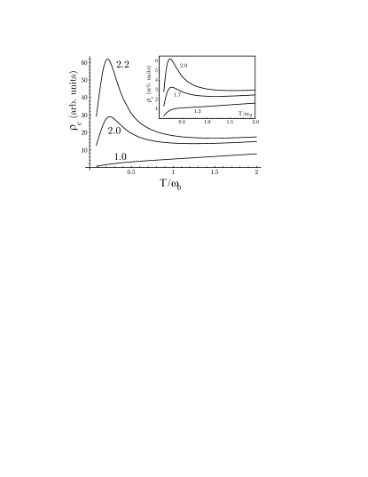
Figure 1: The zero-field $c$-axis resistivity with in-plane marginal Fermi liquid scattering $\Gamma=\omega\coth\left(\omega/T\right)$ for electrons coupled to $c$-axis Einstein phonons for different values of electron-phonon coupling $(\Delta/\omega_{0})$. Inset: as above but for a dispersing mode $\omega_{q}=\omega_{0}[1-0.4\cos(q)]$.

For a more general dispersing bosonic mode, $D(\omega,T)$ can be calculated approximatelymahan_1990a assuming strong electron-phonon interactions. Using the usual approximation $[n_{F}(\nu)-n_{F}(\nu+\omega)]/\omega\simeq-\partial n_{F}/\partial\nu\simeq\delta(\nu)$ valid at low $T$ when $\Gamma(T,\omega)$ varies slowly, we find

$$\sigma_{c}(T,B)=\frac{e^{2}Nt_{c}^{2}}{\pi cT}e^{-C(T)}\int\frac{d\nu}{\sqrt{\pi\gamma^{2}(T)}}\frac{\nu}{\sinh\frac{\nu}{2T}}$$

$$\times{\rm Re}\frac{\exp\left(-\frac{\nu^{2}}{4\gamma^{2}(T)}\right)}{\left[(v_{\rm F}q_{B})^{2}-(\nu+2i\Gamma(T,\nu))^{2}\right]^{1/2}}\;,$$ (13)

where

$$C(T)=\sum_{q}F_{q}\frac{2\sinh^{2}\left(\frac{\omega_{q}}{4T}\right)}{\sinh\frac{\omega_{q}}{2T}},\quad\gamma^{2}(T)=\sum_{q}\frac{F_{q}|\omega_{q}|^{2}}{2\sinh(\omega_{q}/2T)}\;,$$

and $F_{q}=\left|\frac{M_{q}}{\omega_{q}}\right|^{2}2(1-\cos q)$.

For illustration, we consider $\omega_{q}=\omega_{0}[1-0.4\cos(q)]$, and set the electron-phonon coupling $M_{q}$ to be $q$-independent. Eq. 13 is then evaluated numerically and plotted in the inset to Fig. 1. $\bar{\Delta}=\sum_{q}F_{q}\omega_{q}/2$ characterizes the strength of the electron-phonon interaction in this case. The result is qualitatively similar to that of a non-dispersing mode.

Now we consider the magnetic field dependence of the conductivity for the Einstein mode. At low temperatures $T\ll\omega_{0}$ we find that the magnetoresistance reflects the usual cross-over from quadratic to linear field dependence schofield_2000a at a scale determined only by the in-plane electron scattering rate

$$\Delta\rho_{c}={[\rho_{c}(B)-\rho_{c}(0)]/\rho_{c}(0)}=\sqrt{1+[\omega_{c}/2\Gamma(T,0)]^{2}}\;,$$ (14)

where $\omega_{c}=v_{F}ecB$ is the cyclotron frequency. At higher temperatures ($T\gtrsim\omega_{0}$), the weak-field magnetoresistance is quadratic in field $\Delta\rho_{c}\propto(\omega_{c}/\Gamma_{\rm eff})^{2}$ , and defines a new scattering rate, $\Gamma_{\rm eff}$, depending on both the electronic scattering and the phonon frequency. Taking into account only up to $n=1$ harmonics, with $\Gamma_{0}=\Gamma(T,0)$, and $\Gamma_{1}=\Gamma(T,\omega_{0})$, we find

$$\Gamma_{\rm eff}^{2}\approx\frac{\frac{1}{2\Gamma_{0}}+\frac{4\Gamma_{1}}{4\Gamma_{1}^{2}+\omega_{0}^{2}}}{\frac{1}{16\Gamma_{0}^{3}}+\frac{2\Gamma_{1}(4\Gamma_{1}^{2}-3\omega_{0}^{2})}{(4\Gamma_{1}^{2}+\omega_{0}^{2})^{3}}}\;.$$ (15)

As for the zero field resistivity, the magnetoresistance for the dispersing mode case is qualitatively similar to that for the Einstein mode and is positive for all temperatures.

We now consider in more detail how this model might apply to real materials and, in particular, the ruthenate systems. The 2D electronic nature of these materials reflects the crystal structure and so it is natural that the electron-phonon interaction should be anisotropic. While there are to date no calculation for the electron-phonon interaction parameters for the ruthenates, in the iso-structural LSCO cuprate family, Krakauer et. al.Krakauer_1993 have calculated that there is a strong electron-phonon coupling only for modes corresponding to atomic displacements perpendicular to the Cu-O plane, (partly) because of weak screening of the resulting electric fields in this direction. Moreover it has been argued that in the perovskite structure the coupling to c-axis vibrations is enhanced kornilovitch_1999a . There exist optical phonons with the appropriate symmetry for $c$-axis transportBraden in $\rm Sr_{2}RuO_{4}$, and experimentally the broad maximum in the $c$-axis resistivity has been linked to a structural phase transitionjin_2001a in $\rm Ca_{1.7}Sr_{0.3}RuO_{4}$ at around the broad maximum temperature. Thus one should consider the possibility of electron-phonon interaction affecting the $c$-axis transport. In particular, both the $\rm Sr_{2}RuO_{4}$ and $\rm Ca_{1.7}Sr_{0.3}RuO_{4}$ systems exhibittyler_1998a ; jin_2001a qualitatively this broad maximum structure found in our simple model, in the $c$-axis resistivity near to their characteristic ($c$-axis) phonon energy.

Figure 2: Fitting the zero-field $c$-axis resistivity to the data of Tyler et.al. tyler_1998a . See the text for the explanation of the theoretical curve (thin line) and the parameters used for the fitting. The data are plotted as points: for clarity, we have plotted only $3\%$ of the total number of available data points.

A full quantitative modeling of $\rm Sr_{2}RuO_{4}$ is beyond the scope of the simplified model presented here. Despite all these simplifying assumptions, our model does a reasonable fit to the resistivity data of $\rm Sr_{2}RuO_{4}$ as we shall show, perhaps indicating some degree of universality of the mechanism for c-axis transport studied in this paper. Here for reference, we list the simplifications we have assumed in our modeling: 1) the in-plane scattering rate can be deduced directly from $\rho_{ab}$, 2) the main interlayer coupling is single particle hopping from one layer to another and 3) a simple phonon dispersion is employed (see later).

For 1), this amounts to ignoring vertex corrections to in-plane transport. In Fermi liquids, the vertex correction leads to an extra cosine of the angle between in- and out-going electrons thereby correctly penalizing back-scattering in conductivity. However, the qualitative trend is still correct. As mentioned already, we have taken an in-plane spectral function that has no in-plane momentum dependence. This ignores the complicated multiple Fermi surfaces in $\rm Sr_{2}RuO_{4}$. For 2), this means we ignore interlayer coulomb interaction. Also, we ignored the multiband nature of $\rm Sr_{2}RuO_{4}$ and the dependence of $t_{\perp}$ on in-plane momenta. For 3), we have taken the limiting case of an optical phonon mode where the atomic displacements are perpendicular to the plane, and all the atoms in the plane move together. We envisage that just as in LSCO, there will be strong electron-phonon coupling only for phonons propagating mainly in the $c$ directionKrakauer_1993 . Now in reality, because of the non-trivial perovskite structure of $\rm Sr_{2}RuO_{4}$, these modes that can affect $c$-axis transport will have relative atomic displacements both in-plane and out of plane. But this makes electron hopping from one to another plane even more difficult, as the polaron has to create disturbances both in-plane and out-of-plane.

To some extent, these simplifying assumptions may only lead to some quantitative changes in the fit parameters, because the calculation of $\rho_{c}$ (Eq. 7) involves an integral over in-plane momenta and thus averages out such dependences.

We now show in Fig. 2 a fit to the $\rm Sr_{2}RuO_{4}$ data of Tyler et al. tyler_1998a . The theoretical curve is the thin continuous line, the data are the points. The theoretical curve is generated as follows: the in-plane scattering rate is approximated as being proportional to the in-plane $\rho_{ab}$ (also taken from the data of [ tyler_1998a, ]): $\Gamma(T,\omega)\approx A\left(\rho_{ab}(T)+\rho_{0}\right)$, where $A$ and $\rho_{0}$ are fitting parameters. We take a simple optical boson dispersion $\omega(q)=\omega_{0}\left(1-\lambda\cos q\right)$ with the boson bandwidth $\lambda$ and the characteristic energy $\omega_{0}$ as fitting parameters. $\Gamma(T,\omega)$ and $\omega(q)$ are then fed into Eq. 13, where the overall scale of $\rho_{c}$ is found by fitting $\rho_{c}^{\rm max}\sim 33$m$\Omega$ cm to the peak of the theory curve. Despite the simplicity of the model and the lack of knowledge of the exact boson dispersion form, the theory curve is almost indistinguishable from the data points, except at high $T$. The fitting is relatively insensitive to the precise values of the parameters: some fine tuning (mainly, $\lambda$ and $\bar{\Delta}$) is needed to get the positions of the maximum, minimum and final upturn correctly. Furthermore, the parameters used are physically plausible: $\lambda\approx 0.67,\omega_{0}\approx 515$K, $\bar{\Delta}/\omega_{0}\approx 1.4,A/\omega_{0}\approx 0.1($m$\Omega$ cm$)^{-1},\rho_{0}\approx 0.17$ m$\Omega$ cm. The value of $\omega_{0}$ is consistent with the available phonon data of Braden et.al.Braden , while the size of the boson bandwidth suggests that the bosons do disperse in the interplane direction. Note that the dispersion $\omega(q)$ always enter the conductivity expression under a $q$-integral (see Eq.13), and is the reason why our simplified boson dispersion can still model the broad maximum in the $c$-axis resistivity successfully. The size of the electron-boson coupling parameter $\bar{\Delta}$ indicate that ${\rm Sr_{2}RuO_{4}}$ is just slightly above threshold for obtaining the maximum in $\rho_{c}$.

The $c$-axis magnetoresistance seen in ${\rm Sr_{2}RuO_{4}}$ is unusual hussey_1998a , becoming negative for both transverse ($B||ab$) and longitudinal ($B||c$) fields above 80K and maximally so at around 120K—coinciding with the peak position. In this paper we have only considered orbital magnetoresistance and, as might be expected, found it to be positive footnote . This is not inconsistent with the data since the transverse magnetoresistance is always less negative than the longitudinal one. If the change of sign is linked to the origin of the resistivity maximum then, within the framework presented here, it indicates that the frequency of, or coupling to, the bosonic mode is field dependent. At present, we have no microscopic picture of how this might occur.

In conclusion, we have shown that $c$-axis transport in a quasi-2D metal does not always probe only the in-plane electron properties. Strong coupling between electrons and a bosonic mode polarized in the $c$-direction in a highly anisotropic metal can lead to a broad maximum—an apparent metallic to non-metallic crossover—in the $c$-axis resistivity with no corresponding feature in the $ab$ plane properties. The position in the temperature axis, and the shape of this broad maximum are determined mainly by boson parameters and not on the magnitude of the in-plane scattering rate. We have discussed the potential application of the model to $\rm Sr_{2}RuO_{4}$ and its relative $\rm Ca_{1.7}Sr_{0.3}RuO_{4}$. Despite certain simplifying features of the model, the qualitative (and even quantitative) properties of this crossover in these layered ruthenates are captured succinctly.

We are pleased to acknowledge useful and stimulating discussions with M. Braden, C. Hooley, V. Kratvsov, P. Johnson, M. W. Long, Y. Maeno, A. P. Mackenzie, G. Santi, I. Terasaki and Yu Lu. A.F.H. was supported by ICTP, Trieste where this work was initiated, and by EPSRC (UK). A.J.S. thanks the Royal Society and the Leverhulme Trust for their support.

References

- (1) I. Ito, H. Takagi, S. Ishibashi, T. Ido, and S. Uchida, Nature 350(6319), 596 (1991).
- (2) A. W. Tyler, A. P. Mackenzie, S. NishiZaki, and Y. Maeno, Phys. Rev. B 58(16), 10107 (1998).
- (3) J. Singleton, Rep. Prog. Phys. 63, 1111 (2000).
- (4) N. Kumar and A. M. Jayannavar, Phys. Rev. B 45(9), 5001 (1992).
- (5) R. H. McKenzie and P. Moses, Phys. Rev. Lett. 81(20), 4492 (1998).
- (6) K. G. Sandeman and A. J. Schofield, Phys. Rev. B 63, 094510 (2001).
- (7) P. W. Anderson, The theory of superconductivity in the high- cuprates (Princeton University Press, Princeton, New Jersey, USA, 1997).
- (8) M. A. H. Vozmediano, M. P. LopezSancho, and F. Guinea, Phys. Rev. Lett. 89, 166401 (2002).
- (9) P. B. Littlewood and C. M. Varma, Phys. Rev. B 45(21), 12636 (1992).
- (10) L. B. Ioffe and A. J. Millis, Science 285(5431), 1241 (1999).
- (11) A. G. Rojo and K. Levin, Phys. Rev. B 48(22), 16861 (1993).
- (12) M. Turlakov and A. J. Leggett, Phys. Rev. B 63, 064518 (2001), eprint cond-mat/0005329.
- (13) I. G. Lang and Y. A. Firsov, Sov. Phys. JETP 16, 1301 (1963).
- (14) C. Bergemann, et. al. Phys. Rev. Lett. 84, 2662 (2000).
- (15) H. Krakauer, W. E. Pickett, and R. E. Cohen, Phys. Rev. B 47(2), 1002 (1993).
- (16) J. H. Kim, K. Levin, and R. Wentzcovitch, Phys. Rev. B 40(16), 11378 (1989).
- (17) M. Grilli, and C. Castellani, Phys. Rev. B 50(23), 16880 (1994).
- (18) T. Holstein, Ann. Physics 8, 343 (1959).
- (19) G. D. Mahan, Many-Particle Physics (Plenum Press, New York, 1990), 2nd ed.
- (20) P. E. Kornilovitch, Phys. Rev. 59(21), 13531 (1999).
- (21) U. Lundin and R. H. McKenzie, Phys. Rev. B 68, 081101 (2003), eprint cond-mat/0211612.
- (22) A. Altland, C. H. W. Barnes, F. W. J. Hekking, and A. J. Schofield, Phys. Rev. Lett. 83(6), 1203 (1999), eprint cond-mat/9907459.
- (23) A. F. Ho and A. J. Schofield, Small polarons and c-axis transport in highly anisotropic metals, eprint cond-mat/0211675.
- (24) This implies that even if at very high temperatures, becomes independent of , the resistivity will not saturategunnarsson_2003a ; hussey_2004a .
- (25) O. Gunnarsson, M. Calandra, and J. E. Han, Rev. Mod. Phys. 75, 1085 (2003).
- (26) N. E. Hussey, K. Takenaka, and H. Takagi, Universality of the Mott-Ioffe-Regel limit in metals, eprint cond-mat/0404263.
- (27) A. J. Schofield and J. R. Cooper, Phys. Rev. B 62(16), 10779 (2000), eprint cond-mat/9709167.
- (28) For LSCO, where the parent compound is isostructural to , the mode that can couple to -axis transport is the axial mode, at ). It has the strongest electron-phonon coupling in the whole zone and behaves like an Einstein phonon: C. Falter, M. Klenner, and W. Ludwig, Phys. Rev. B 47, 5390, (1993); H. Krakauer, W.E. Pickett, and R.E. Cohen, Krakauer_1993 . A similar mode has been seen in inelastic neutron scattering in , M. Braden et al., unpublished and personal communication.
- (29) R. Jin, J. R. Thompson, J. He, J. M. Farmer, N. Lowhorn, G. A. Lamberton, Jr., T. M. Tritt, and D. Mandrus, Heavy-electron behavior and structural change in Ca1.7Sr0.3RuO4, eprint cond-mat/0112405.
- (30) N. E. Hussey, A. P. Mackenzie, J. R. Cooper, Y. Maeno, S. Nishizaki, and T. Fujita, Phys. Rev. B 57(9), 5505 (1998).
- (31) It is possible to obtain a negative orbital magnetoresistance within this model. It requires either a phonon function that peaks at a finite frequency, or an in-plane spectral weight where the scattering rate is smallest at a finite frequency. Either of these possibilities suppress the contribution to (see Eq. 9.) Intriguingly, after this work was completed, we learnt from P. Johnson that the in-plane spectral weight near and above may be anomalous, in contrast to the spectral weight observed in the low temperature Fermi liquid state. Work is in progress to take this into account within the present framework.