Models of coherent exciton condensation

Abstract

That excitons in solids might condense into a phase-coherent ground state was proposed about 40 years ago, and has been attracting experimental and theoretical attention ever since. Although experimental confirmation has been hard to come by, the concepts released by this phenomenon have been widely influential. This tutorial review discusses general aspects of the theory of exciton and polariton condensates, focussing on the reasons for coherence in the ground state wavefunction, the BCS to Bose crossover(s) for excitons and for polaritons, and the relationship of the coherent condensates to standard lasers.

1 Introduction

An electron and a hole optically excited within a solid are oppositely charged, and bind together to form a bosonic exciton. Since the mass of this particle is typically small, there has long been interest in the possibility of obtaining a Bose-Einstein condensate (BEC) at cryogenic temperatures[1, 2, 3]. Experimentally this has proved challenging, because excitons are not the ground state of the system, and a cold equilibrium gas needs to be prepared on a shorter time scale than the excitons can decay. There have been many approaches to this problem (for some reviews see [4, 5, 6]) with particularly important systems being $\mathrm{Cu_{2}O}$ [7] (where dipole- and spin-forbidden transitions are harnessed to produce excitons with long lifetimes) $\mathrm{CuCl}$ [9] (which has very stable biexcitons) and two-dimensional coupled quantum wells (where electrons and holes are physically separated by a tunnel barrier)[10, 12, 14, 15, 16].

In a situation where the dominant decay mechanism is by dipole radiation, the opportunity to confine the light inside an optical microcavity[17] allows one instead to work with the coupled eigenstates of the electron-photon problem, namely polaritons[18]. The polariton effective mass can be made much lighter – as small as $10^{-5}$ of the electron mass – and a naive estimate of the critical temperature thus even higher. One now has an extra handle on the experimental system because coupling of the cavity to an external electromagnetic field allows both coherent and incoherent pumping of the system. Some recent work has demonstrated the onset of stimulated emission[19, 20], parametric oscillation in a driven cavity[21] as well as the development of spontaneous[22, 23, 24] optical coherence in semiconductor microcavities.

This article will review some of the theoretical aspects of the exciton problem, particularly associated with the construction of an appropriate wavefunction for a condensate that is based on bound pairs of fermions. The basic insight on this problem was provided by the work of Keldysh and collaborators[3, 25] using a variational wavefunction in close analogy to the BCS wavefunction for superconductivity. This approach was extended by Nozières and Comte[26] who showed how such a wavefunction smoothly interpolates between the regime of a dilute Bose gas and a dense two-component plasma, and then reworked for superconductors to provide a theory of the BCS-BEC crossover[29, 30]. We will explain here how the collective mode spectrum changes qualitatively between the two limits, and connect this spectrum to the familiar picture of a dilute Bose gas.

In the polariton condensate, the pairs of fermions can resonantly decay into photons, so the order parameter is shared between the two coherent degrees of freedom – the photon electric field and the excitonic polarisation. Inspection of this physical system also reminds us that BEC in an interacting system leads to a broken symmetry corresponding to phase coherence of the dipole oscillators – so that in a broad sense BEC of polaritons makes a kind of laser. To make that relationship explicit, we shall discuss the Dicke model of localised dipole-active transitions coupled to a cavity field. It turns out that a straightforward generalisation of the BCS-like wavefunction for the coupled system provides a good description of the problem[31, 32]. This mean field theory can be extended[33] to discuss the analog of the BCS-BEC crossover – which in this case connects the limits of BEC of a dilute gas of polaritons with a higher density system where the coherence is produced through the self-consistent optical field (as in a laser). It turns out that the density scale for this crossover corresponds to a separation between excitons(i.e. excitations of the localised transitions) which is the geometric mean of two parameters: the wavelength of photons at energies of the order of the polariton splitting, and the spatial separation of the localised transitions. The former length scale is generally a few tenths of a micron, while the latter is greater than the exciton Bohr radius. Thus the density range where the correct description of the problem is polaritonic BEC is probably quite limited.

The model we use for polaritonic condensation is similar to that describing other systems based on (quantum) oscillators coupled by resonance with a bosonic field[34]: two prominent examples are arrays of small Josephson junctions coupled in a microwave cavity[35, 36], and cold fermionic atoms coupled to a molecular Feshbach resonance[37, 38]. The phase-coherent ground state describing the excitonic insulator can be mapped to the coupled bilayer quantum Hall state near $\nu=1/2$ [39, 40].

We shall stress that the important issue associated with excitonic or polaritonic condensation is coherence, rather than momentum condensation as in the weakly interacting Bose gas. Because we are dealing with physical systems that are open, and can exchange excitation with the environment, the coherence in the system may be destroyed not only thermally by internal excitations (i.e. particle-hole pairs or phase fluctuations) but also by coupling to external baths (which may be non-thermal). These decoherence processes can produce crossovers to other, more familiar, coherent phenomena such as lasing, before driving the system into complete incoherence[41, 42, 43].

2 Possible phases of the electron-hole system

The Hamiltonian of the electron-hole system consists of the kinetic energy of the separate components, and the Coulomb interaction between them. Written in second-quantised notation,

$$H=H_{o}+H_{coul},$$ (1)

where

$$H_{o}=\sum_{k}\left[\epsilon_{ck}a_{c,k}^{\dagger}a_{c,k}+\epsilon_{vk}a_{v,k}^{\dagger}a_{v,k}\right],$$ (2)

and

$$H_{coul}=\frac{1}{2}\sum_{q}\left[V^{ee}_{q}\rho^{e}_{q}\rho^{e}_{-q}+V^{hh}_{q}\rho^{h}_{q}\rho^{h}_{-q}-2V^{eh}_{q}\rho^{e}_{q}\rho^{h}_{-q}\right].$$ (3)

$a_{c,k}^{\dagger}$ and $a_{v,k}^{\dagger}$ are creation operators for electrons in the conduction and valence bands. The density operators are $\rho^{e}_{q}=\sum_{k}a_{c,k+q}^{\dagger}a_{c,k}$, $\rho^{h}_{q}=\sum_{k}a_{v,k}a_{v,k+q}^{\dagger}$. $V(q)$ is the Coulomb interaction, and for a homogeneous three-dimensional system $V^{ee}=V^{hh}=V^{eh}=4\pi/\epsilon q^{2}$. It is interesting also to consider the two dimensional situation of separate layers of electrons and holes, where $V^{ee}_{q}=V^{hh}_{q}=2\pi/\epsilon q$, $V^{eh}_{q}=2\pi e^{-qd}/\epsilon q$, and $d$ is the interlayer separation. For parabolic bands, then $\epsilon_{c}(k)=\hbar^{2}k^{2}/2m_{e}$; $\epsilon_{v}(k)=-E_{g}-\hbar^{2}k^{2}/2m_{h}$.

The natural units are the exciton Rydberg, $Ry^{*}=\frac{\mu e^{4}}{2\epsilon^{2}\hbar^{2}}=\frac{\mu}{m}\frac{1}{\epsilon^{2}}Ry$, and the exciton Bohr radius, $a^{*}=\frac{\epsilon\hbar^{2}}{\mu e^{2}}=\epsilon\frac{m}{\mu}a_{o}$. Here $Ry=13.6\;eV$ is the Hydrogenic Rydberg, $\mu$ the reduced mass, and $a_{o}=5\times 10^{-10}\mathrm{m}$ the hydrogenic Bohr radius. One of the principal reasons that semiconductor systems are so interesting is that a combination of small band mass $\mu$ and large dielectric constant $\epsilon$ means that $a^{*}$ can often be very large – so even at moderate excitation levels, the characteristic separation between excitons can be made comparable to their Bohr radius. It is convenient to measure the density $n$ (of electron-hole pairs) of the system in units of the Bohr radius by defining the dimensionless parameter $r_{s}$: in three dimensions $\frac{1}{n}=\frac{4\pi}{3}(r_{s}a^{*})^{3}$, and in two dimensions $\frac{1}{n}=\pi(r_{s}a^{*})^{2}$.

This is not the complete Hamiltonian for electrons and holes in a real solid with a real bandstructure that includes all the effects of Bloch electrons. The model is a good approximation for semiconductors with a light mass and a large dielectric constant because the effective Bohr radius is much longer than the physical lattice constant. Most importantly for our purposes, this Hamiltonian separately conserves the number of electrons and the number of holes. Interband tunnelling and interband exchange is neglected here. This neglect is not quantitatively important for determining the ground state, but if present will break the conservation of electrons and holes and formally prohibit a superfluid ground state[44, 45].

The electron-hole system is surely one of the simplest model systems in condensed matter physics. The ground state(s) of this model are likely to include various kinds of quantum solids and liquids[46]. The relevant parameters are the density (measured by $r_{s}$), the mass ratio of electron to hole $\Gamma=m_{e}/m_{h}$, and, for 2D bilayers, the separation $d$. If $\Gamma\gg 1$, then we are discussing hydrogen, where we expect that the two basic phases are either a molecular solid of $H_{2}$, or at very high densities a metallic crystal — where the electrons delocalise. (There may of course be solid phases with different crystal structures within each of these basic types). The pressures required to obtain this are immense. There is no regime where a gas of individual excitons is expected.

The molecular stability of $H_{2}$ is large — the heat of formation of a molecule from two atoms of hydrogen is roughly 1/3 $Ry$ — which is why the phase diagram at moderate to low densities $r_{s}>1$ should be dominated by solid phases in a system with high hole mass. In contrast, with electron and hole of roughly equal mass the binding energy of the biexciton $X_{2}$ — the analogue of $H_{2}$ — is about one order of magnitude smaller, and the biexcitonic molecule is corresponding large. In consequence, the biexcitonic solid (nearly equal masses) is expected to form (if at all) only at low densities ($r_{s}\approx 5-10$). At higher densities, it is plausible to believe that this solid will melt to form a fluid phase. The form of this quantum fluid is easy to imagine at very high densities $r_{s}\ll 1$, because here the kinetic energy of both species (scaling like $r_{s}^{-2}$) will overcome the Coulomb binding (scaling as $r_{s}^{-1}$) and a good description would be of two interpenetrating Fermi liquids. At lower density, there will be fluctuations leading to the transient appearance of excitonic atoms and molecules in the solid, and these configurations will preponderate at larger $r_{s}$.

There is also the possibility of an exciton crystal, which would be an atomic (Mott) insulator in contrast to the biexcitonic band insulator. Such a phase should be readily stabilised in 2D bilayer systems at large $d$ and small $r_{s}$, where it is more easily recognised as two coupled Wigner crystals. The 2D bilayers should also have reduced stability of the biexciton (because of dipole repulsion between two excitons) and so are more likely to support quantum fluid phases over a wider range of density that 3D systems.

This model is amenable to study by advanced numerical techniques, including variational[47], quantum[48] and path-integral[49] Monte Carlo methods. However, the full phase diagram has not yet been established theoretically.

3 Theory of the excitonic insulator

From now on we shall be concerned entirely with the fluid phase, and immediately the question arises about whether it is condensed. There are three major aspects to the character of a condensate: the statistical physics of bosons (the conventional texbook view of BEC); phase coherence of the order parameter; and superfluidity.

Since at low density, $r_{s}\gg 1$, we have a fluid that can be sensibly thought of as atomic, one expects Bose-Einstein condensation (BEC). Conventionally, one regards BEC as a phenomenon associated with the statistical physics of weakly interacting bosons. While this may be appropriate for a very dilute gas of strongly bound atoms, it is less clear whether this is the appropriate physical description of a dense two-component plasma. So the first issue is how to write down a wavefunction in terms of the fermionic components, that nevertheless recognisably describes bosons in the dilute limit.

Such a wavefunction must contain within it the important physical characteristic of macroscopic phase-coherence. Phase coherence is a consequence of interactions, but even infinitesimally small interactions in boson systems convert the (highly degenerate) ground state obtained by considering the statistical physics of BEC to a robust phase-locked condensate. It turns out that in exciton and polariton systems the phase coherence has physical consequences for the interaction with electromagnetic radiation that are different from in a superconductor and quite characteristic of the condensed state.

The third, and most subtle issue, is that of superfluidity. In an extended fluid with Galilean invariance, continuous changes in the superfluid phase generate supercurrents that can flow without dissipation. Whether or not the exciton condensate is a true superfluid (or instead a density wave) and what in fact would be the correct superfluid response is a subtle topic that is not yet completely resolved.

Before addressing excitonic systems, it is useful to start with a brief review of BEC in the dilute Bose gas (for a general and complete exposition, see e.g. the book by Pethick and Smith[51]). Since the first observation of BEC in cold atomic gases in 1995, there has of course been tremendous activity in this field that we will not attempt to review. Our discussion will be focussed on the effect of interactions and coherence.

3.1 Coherence and interactions in atomic BEC

BEC as a phenomenon in statistical physics is usually presented in terms of the occupancy of single particle states $n_{q}$, indexed by momentum $q$. For a free particle of mass $M$, the states are occupied according to the Bose factor

$$n_{q}=\frac{1}{e^{\beta(E_{q}-\mu)}-1}$$ (4)

where $E_{q}=\hbar^{2}q^{2}/2M$ is the kinetic energy of the boson, and $\beta=1/k_{B}T$. The total number of particles in the system is then fixed by

$$N=\sum_{q}n_{q}=\int dE\frac{D(E)}{e^{\beta(E-\mu)}-1}\;\;\;,$$ (5)

which is actually an equation determining the chemical potential as a function of temperature. Here $D(E)\propto E^{d/2-1}$ is the density of states in dimension $d$.

As temperature is lowered the Bose factor in Eq. (5) becomes sharply peaked in the vicinity of the chemical potential — and in consequence $\mu$ must increase so as to allow the integral to conserve $N$. Remarkably, in dimensions $d>2$ it turns out that the integral remains finite even as $\mu\to 0$, and therefore the chemical potential reaches the bottom of the band at a non-zero temperature $T_{BEC}$. By dimensional arguments it is clear that this temperature is close to the degeneracy temperature $k_{B}T_{o}=\hbar^{2}n^{2/d}/m$, where the thermal de Broglie wavelength reaches the interparticle separation. Below this temperature $\mu$ remains clamped to the bottom of the band and the state with zero momentum has an occupation proportional to the total number of particles $N$ in the system.

3.2 Interactions, broken symmetry and collective modes in the dilute atomic condensate

This picture is not an inaccurate way to describe a dilute gas of weakly interacting bosons, but it misses a crucial feature of BEC — macroscopic phase coherence, and the rigidity of the condensate[52, 53]. If we have a system of macroscopic size $\Omega=L^{d}$ then, as L is very large, there is only a small separation in energy, $\propto L^{-2}$, between the ground state $q_{0}=0$ and the low-lying excited states with momenta $q$ of order $1/L$. So while the number state $|N,q_{0}\rangle=N^{-1/2}(c_{0}^{\dagger})^{N}\left|0\right>$ is indeed lowest in energy, states of the form $(c_{0}^{\dagger})^{N-m_{1}-m_{2}...}(c_{1}^{\dagger})^{m_{1}}(c_{2}^{\dagger})^{m_{2}}...\left|0\right>$ have an energy that is greater only by an amount of order $(m_{1}+m_{2}+...)/L^{2}$, provided we restrict ourselves to momenta of order $1/L$. (We use $c_{k}$ as the annihilation operator for a boson in momentum state $q_{k}$ and $\hat{\phi}({\bf r})=\sum_{k}<{\bf r}|k>c_{k}=\Omega^{-1/2}\sum_{k}\exp(i{\bf k}\cdot{\bf r})c_{k}$ for the field operator.)

What breaks this near degeneracy are interactions between particles. Consider the (bosonic) Hamiltonian $H_{0}+H_{int}$, for particles of mass $m$ in an external potential $V_{ext}$. We have

$$H_{0}=\int d{\bf r}\hat{\phi}^{\dagger}({\bf r})\left[-\frac{\hbar^{2}\nabla^{2}}{2m}+V_{ext}({\bf r})\right]\hat{\phi}({\bf r}),$$ (6)

together with the interaction term

$$H_{int}=\frac{1}{2}\int d{\bf r}d{\bf r^{\prime}}V({\bf r}-{\bf r^{\prime}})\hat{\phi}^{\dagger}({\bf r})\hat{\phi}^{\dagger}({\bf r^{\prime}})\hat{\phi}({\bf r^{\prime}})\hat{\phi}({\bf r}).$$ (7)

(Often this interaction is modelled by a short range term $V({\bf r}-{\bf r^{\prime}})=V_{0}\Omega\delta({\bf r}-{\bf r^{\prime}})$, an approximation which is sensible once the thermal de Broglie wavelength $\lambda_{T}=(2\pi\hbar^{2}\beta/m)^{1/2}$ is much larger than the interparticle spacing — or equivalently that $T\ll T_{o}$.)

We can discuss the effect of the interaction energy using an appropriate trial wavefunction. Rather than the number states $|N,q_{0}\rangle$ we instead consider coherent states

$$|\Lambda,q_{0}\rangle=e^{\lambda c_{0}^{\dagger}}e^{-|\lambda|^{2}/2}|0\rangle.$$ (8)

This wavefunction is a state of well-defined phase, with an expectation value of the number of particles of $\langle N\rangle=|\lambda|^{2}$:

$$\langle\Lambda|\hat{\phi}({\bf r})|\Lambda\rangle=\lambda=|\lambda|e^{i\theta}.$$ (9)

The phase is conjugate to the number of particles since we can generate a number state $\left|N\right>$ as follows:

$$\int d\theta\;e^{-iN\theta}\left|\Lambda,q_{0}\right>\propto\left|N,q_{0}\right>.$$ (10)

To show how the interactions make the system resistant to fragmentation, consider a mixed state

$$\left|\Psi\right>=e^{-\lambda^{2}/2}e^{\lambda(\cos(\alpha)c_{0}^{\dagger}+\sin(\alpha)c_{1}^{\dagger})}\left|0\right>.$$ (11)

This state has a population fragmented between two different momenta: $N_{0}=\lambda^{2}\cos^{2}(\alpha)$, $N_{1}=\lambda^{2}\sin^{2}(\alpha)$, $N_{0}+N_{1}=N$ (here we restrict $\alpha,\lambda$ to be real without loss of generality). The interaction energy can be straightforwardly evaluated

$$\left<\Psi\right|H_{int}\left|\Psi\right>=\frac{1}{2}\lambda^{4}V_{o}[1+\frac{1}{2}\sin^{2}(2\alpha)]=\frac{1}{2}V_{o}N^{2}+V_{o}N_{0}N_{1}.$$ (12)

Since $V_{o}$ is positive (repulsive interactions) the energy is clearly minimised by the pure state with $\alpha=0$ or $\alpha=\pi/2$; which of these two is lowest is determined by the kinetic energy. Notice that this answer does not depend on the momenta of the two states (as long as they are both small). The interaction energy provides an extensive energy penalty for any mixture, as long as the interactions are repulsive.

The coherent states (8) and (11) are often described as “breaking global gauge symmetry”, in that they have a well-defined overall phase. This feature, however, is not essential for the arguments above. We could have reached an identical conclusion using number states, which do not have an overall phase, because to leading order in $N$ the energy of (8) is identical to that of $|N,q_{0}\rangle$, and the energy of (11) is identical to that of $|N_{0},q_{0};N_{1},q_{1}\rangle$. The point is that a single state in an interacting system has a particular phase relationship between different components of the wavefunction. In a condensate, the energy differences between states with different phase relationships can be large, even when the matrix elements are small, because statistics ensures that some modes become macroscopically occupied. Thus phase relationships which in the normal state are washed out by thermal fluctuations, or by applied fields, become robust in the condensed state.

The generally accepted definition of a Bose condensate is as a system with off-diagonal long-range order[54]. This means that the one-body density matrix, $\langle\hat{\phi}^{\dagger}({\bf r})\hat{\phi}({\bf r}^{\prime})\rangle$, approaches a non-zero constant for large separations $|{\bf r}-{\bf r}^{\prime}|$. The practical upshot of this is that one can see interference effects between particles removed from widely separated regions of the condensate, so that off-diagonal long-range order is indeed connected to the presence of unusual phase relationships in the wavefunction. Interestingly, interactions in condensates should enforce phase relationships involving more than two removed particles[53], although the presence of such higher-order coherence is not required by the definition of off-diagonal long-range order. Note also that standard wavefunctions, such as (8), often contain higher orders of coherence than required for the presence of off-diagonal long-range order.

To understand the collective behaviour of a condensate we need to introduce an order parameter for condensation. One way to do this is to define the order parameter from the one-body density matrix according to $\langle\hat{\phi}^{\dagger}({\bf r})\hat{\phi}({\bf r}^{\prime})\rangle=\phi^{\ast}({\bf r})\phi({\bf r}^{\prime})$. This defines the order parameter $\phi({\bf r})$, which is a complex classical field called the condensate wavefunction. The Ginzburg-Landau free energy for the condensate wavefunction $\phi({\bf r})$ is

$$F[\phi]=\int d{\bf r}\left[\frac{\hbar^{2}}{2m}\left|\nabla\phi({\bf r})\right|^{2}+(V_{ext}({\bf r})-\mu)|\phi({\bf r})|^{2}+\frac{V_{o}}{2}\left|\phi({\bf r})\right|^{4}\right]$$ (13)

The formal route to this functional constructs an action based on the model of interacting bosons above, from which the G-L theory emerges as a classical saddle point (see, e.g.[55]). The path from here on is discussed in many textbooks[51], and we will just quote results.

If we minimise the free energy of Eq. (13) we obtain an equation for the ground state wavefunction $\phi_{o}$ which is the Gross-Pitaevski equation

$$\left[-\frac{\hbar^{2}}{2m}\nabla^{2}+V_{ext}({\bf r})-\mu+V_{o}\left|\phi_{o}({\bf r})\right|^{2}\right]\phi_{o}({\bf r})=0.$$ (14)

If we now consider small deviations $\phi=\phi_{0}+\eta$, then we can determine the energy of quadratic fluctuations:

$$\int d{\bf r}\left(\begin{array}[]{c c}\eta^{*}&\eta\end{array}\right)\left(\begin{array}[]{c c}-\frac{\hbar^{2}}{2m}\nabla^{2}+V_{ext}-\mu+2V_{o}|\phi_{o}|^{2}&+V_{o}\phi_{o}^{2}\\ +V_{o}\phi_{o}^{*2}&-\frac{\hbar^{2}}{2m}\nabla^{2}+V_{ext}-\mu+2V_{o}|\phi_{o}|^{2}\end{array}\right)$$ (18)

$$\times\left(\begin{array}[]{c}\eta\\ \eta^{*}\end{array}\right).$$ (21)

The fluctuations mix the real and imaginary components of the fields: what is happening is simplest to envisage for a uniform condensate ($V_{ext}=0$); then the solution of Eq. (14) determines the chemical potential $\mu=V_{0}|\phi_{o}|^{2}=V_{o}n_{o}$, and after taking a Fourier transformation the matrix at the core of Eq. (21) becomes

$$\left(\begin{array}[]{c c}\epsilon_{k}+V_{o}|\phi_{o}|^{2}&V_{o}\phi_{o}^{2}\\ V_{o}\phi_{o}^{*2}&\epsilon_{k}+V_{o}|\phi_{o}|^{2}\end{array}\right),$$ (22)

where $\epsilon_{k}=\hbar^{2}k^{2}/2m$. Since we have a coupling between $\eta$ and $\eta^{*}$, not only is the normal average $<\eta\eta^{*}>$ non-zero, but also the anomalous average $<\eta\eta>$. Note that when we determine the dynamics of the new wavefunctions, i.e. turning Eq. (21) into a Schrödinger equation, we need to get the time dependence straight by looking for solutions of the form $(\eta^{\ast}\;\;\eta)=(\eta_{0}^{\ast}e^{i\omega_{k}t}\;\;\eta_{0}e^{-i\omega_{k}t})$. This leads to an eigenvalue spectrum determined by

$$\left(\begin{array}[]{c c}-\omega_{k}+\epsilon_{k}+V_{o}|\phi_{o}|^{2}&V_{o}\phi_{o}^{2}\\ V_{o}\phi_{o}^{*2}&+\omega_{k}+\epsilon_{k}+V_{o}|\phi_{o}|^{2}\end{array}\right).$$ (23)

The new excitation modes of the condensate thus have the dispersion first derived by Bogoliubov

$$\omega_{k}=\sqrt{\epsilon_{k}^{2}+2V_{o}n_{o}\epsilon_{k}}.$$ (24)

This spectrum is acoustic in the long-wavelength limit $k\xi\ll 1$, where $\xi=\hbar/(2mn_{o}V_{o})^{1/2}$ is the healing length. One may also easily check that in the long wavelength limit this mode descibes fluctuations of the phase of the order parameter, as we expected.

This approach connects the microscopic theory to the insight of Landau that a fluid with only phonons as the low energy excitation spectrum cannot absorb arbitrarily small amounts of energy whilst also conserving momentum. The coherence in the underlying wavefunction generated an acoustic spectrum, and that produces superfluidity.

3.3 Mean field theory for excitons

Now we return to the consideration of exciton systems, and our first concern is to write down an analogous wavefunction for BEC, when our bosons consist of bound pairs of fermions.

The wavefunction for a single exciton is just a wavepacket of electron-hole pairs, viz.

$$\left|\Phi_{q}\right>=\sum_{k}\phi(k,q)a_{c,k+q}^{\dagger}a_{v,k}\left|0\right>,$$ (25)

Here our vacuum state $|0\rangle$ is a filled valence band and empty conduction band; consequently $a_{v,k}$ creates a valence band hole. Eq. (25) describes an exciton with centre of mass momentum $q$, and $\phi(k,0)$ is thus just the Fourier transform of the real space exciton wavefunction in relative coordinates. This is manifestly not a boson, but let us write a coherent state in analogy to Eq. (8) as follows:

$$|\Psi_{MF}>=e^{\lambda\sum_{k}\phi(k,0)a_{c,k}^{\dagger}a_{v,k}}\left|0\right>.$$ (26)

Writing a wavefunction with fermion operators in the exponential is not necessary, because unlike bosons, we cannot have two fermions in the same state. So we can manipulate this wavefunction into something more familiar. We generalise the hydrogenic state to a variational function $g(k)$ and then expand the exponential, noting that the series terminates after the second term:

$$|\Psi_{MF}> = \prod_{\vec{k}}e^{g(k)a_{c,k}^{\dagger}a_{v,k}}\left|0\right>$$ (27)

$$= \prod_{\vec{k}}[u_{\vec{k}}+v_{\vec{k}}a_{c,k}^{\dagger}a_{v,k}]|0\rangle.$$

In the last line we have written $g(k)=v(k)/u(k)$ and have normalised the wavefunction so that $|u_{k}|^{2}+|v_{k}|^{2}=1$. $v(k)$ may now be taken as a variational function, and this wavefunction was written down by Keldysh and Kopaev[3] in complete analogy to the BCS theory of superconductivity.

Provided $v_{k}$ (in general complex) has the same phase for all momenta this is a coherent state in the same sense as the bosonic state. But this wavefunction is in general richer than for bosons, as it has an explicitly fermionic description and a variational function $v_{k}$.

3.4 BCS to BEC crossover for excitons

The variational functions $u(k)$ and $v(k)$ should be evaluated by minimising the expectation value of the Coulomb Hamiltonian, Eq. (1). The details have been discussed in many places and for many different geometries, for example by [26, 45], and we will just review the main results. Just as in a BCS model of superconductivity, we have an order parameter corresponding to the broken gauge symmetry (phase coherence), and a gap in the excitation spectrum.

In order to control the density, we introduce the chemical potential $\mu$ for the introduction of electron-hole pairs with density $n$. We then minimize the free-energy

$$F=<H_{o}+H_{Coul}>-\mu<n>,$$ (28)

with respect to the variational parameters $v_{k}$. Setting $\partial F/\partial v_{\vec{k}}=0$ and considering only $s$-wave pairing in which case all quantities are functions of $k$, the magnitude of $\vec{k}$, one gets a BCS-like set of self-consistent equations [26, 56]:

$$\xi_{k} = \epsilon_{k}-\mu-2\sum_{k^{\prime}}V^{ee}_{k-k^{\prime}}n_{k^{\prime}}=\epsilon_{k}-\mu-\sum_{\vec{k}^{\prime}}V^{ee}_{k-k^{\prime}}(1-\xi_{k^{\prime}}/E_{k^{\prime}}),$$ (29)

$$\Delta_{k} = 2\sum_{k^{\prime}}V^{eh}_{k-k^{\prime}}<a_{c,k}^{\dagger}a_{v,k}>=\sum_{k^{\prime}}V^{eh}_{k-k^{\prime}}\Delta_{k^{\prime}}/E_{k^{\prime}},$$ (30)

$$E_{k}^{2} = \xi^{2}_{k}+\Delta^{2}_{k}.$$ (31)

Here Eq. (29) gives the renormalized single-particle energy (per pair) $\xi_{k}$ measured from the chemical potential.($\epsilon_{k}=\frac{k^{2}}{2m_{e}}+\frac{k^{2}}{2m_{h}}$.) Eq. (30) is the “gap equation”, familiar from BCS, so $\Delta_{k}$ is the gap-function and is also the order-parameter. Note that in order for $\Delta$ to exist both $u$ and $v$ must be non-zero for some overlapping range of momenta $k$; this function describes the overall degree of phase-coherence. $E_{k}$ can be identified as the pair-breaking excitation spectrum: it is the energy cost of taking one pair out of the condensate and placing them in plane-wave states of momentum $\vec{k}$.

The BCS ansatz is exactly equivalent to a Hartree-Fock approximation, allowing for the possible (self-consistent) expectation value of an off-diagonal self-energy term. The spectrum of Eq. (31) can be seen as arising from the action

$$\left(\begin{array}[]{c c}a_{c,k}^{\dagger}&a_{v,k}^{\dagger}\end{array}\right)\left(\begin{array}[]{c c}\omega-\frac{1}{2}\xi_{k}&\frac{1}{2}\Delta^{*}_{k}\\ \frac{1}{2}\Delta_{k}&\omega+\frac{1}{2}\xi_{k}\end{array}\right)\left(\begin{array}[]{c}a_{c,k}\\ a_{v,k}\end{array}\right)$$ (32)

If the density is low, $r_{s}\gg 1$, then the isolated excitons are expected to overlap very little. Hence we expect that $v_{k}\ll 1$, and $u_{k}\approx 1$ so that the wavefunction has the approximate form

$$|\Psi_{MF}>\stackrel{{\scriptstyle r_{s}\to\infty}}{{\rightarrow}}\prod_{\vec{k}}\frac{1+\lambda\phi(k,0)a_{c,k}^{\dagger}a_{v,k}}{\sqrt{1+\lambda^{2}\phi(k,0)^{2}}}\left|0\right>$$ (33)

where $\lambda\propto n^{1/2}\propto r_{s}^{-1}$ is now small. In this limit $\mu<0$ (we measure energies from the bottom of the combined electron and hole bands) and approaches -1 Rydberg as the density becomes infinitesimal – just the binding energy of the electron-hole pair. The lowest excitation energy of the system occurs at $k=0$, and corresponds to the ionisation of an exciton into a free electron-hole pair.

In the opposite limit of high density where the electron and hole kinetic energy dominate the interaction energy, we should expect to find a ground state consisting of two interpenetrating Fermi liquids, i.e.

$$|\Psi_{MF}>\stackrel{{\scriptstyle r_{s}\to 0}}{{\rightarrow}}\prod_{|{{\bf k}}|<k_{F}}a_{c,k}^{\dagger}a_{v,k}\left|0\right>.$$ (34)

So for $r_{s}\ll 1$ we expect that $v_{k}=\Theta(|k|-k_{F})$, where $k_{F}$ is the Fermi momentum of the occupied electrons (or holes). So here $\mu=\epsilon_{k_{F}}$ and is positive – within the bands. In the extreme limit $r_{s}\to 0$ the order parameter vanishes; for small, non-zero $r_{s}$, the model can be explicated in terms of a Fermi surface instability. Here, the effect of the Coulomb interaction is confined only to states close to the Fermi surface, producing a small rounding of the occupation functions away from those of the free Fermi gas. The order parameter $\Delta_{k}$ is small (in comparison to $\mu$) and generated mostly by states whose momenta are within $\Delta_{k_{F}}/v_{F}$ of the Fermi wavevector, $v_{F}=\partial\epsilon/\partial k$ being the Fermi velocity. The minimum excitation energy equals $\Delta_{k_{F}}$, and involves breaking pairs whose components have momenta near to the Fermi surface.

As an example of how this works in practice, Fig. 1 shows the evolution of the variational wavefunction from low to high density, calculated for a bilayer electron-hole system [45]. The trends we have described above are quite clear, so this ground state wavefunction apparently does a good job with the oft-called BCS to BEC crossover, with, however, a wavefunction that is always of the same form.

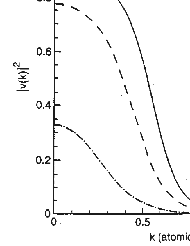
Figure 1: Occupancy $v(k)^{2}$ of the variational wavefunction at low and high densities. Note how it evolves from nearly a Fermi function at small $r_{s}$ to a Lorentzian form (expected for a hydrogenic exciton) at low density. Dotted line: $r_{s}=2.11$; thick solid line: $r_{s}=3.69$; dashed line: $r_{s}=4.72$; dotted-dashed line: $r_{s}=9.56$. The calculations are for coupled quantum wells at a separation of 1 Bohr radius. From [45].

Along with the change in wavefunction, the energy spectrum changes also. In Fig. 2 we show a qualitative sketch of the behaviour of the parameters of the theory as a function of $r_{s}$. (A particular calculation for 2D bilayer systems is given in [45], which confirms the trends shown here, though details may differ – in particular $E_{min}$ may have a weak maximum near the point where the chemical potential passes through the bottom of the band.) As $r_{s}$ increases see that the chemical potential ($\propto 1/r_{s}^{2}$ in the plasma) drops below the bottom of the free electron-hole band, reaching eventually $-1$ Rydberg as $r_{s}\to\infty$. The ground state energy per particle tends also to the same value, as we expect. Near to where $\mu$ crosses the band edge the quasiparticle-hole excitation spectrum changes its form, as the minimum excitation energies go from being near to the Fermi wavevector $k_{F}$ to being at $k=0$. The latter excitations correspond just to the unbinding of an exciton into free particles and holes (see Figure 3). In the high density limit, the gap parameter $\Delta(k_{min})$ and $E_{min}$ are the same. In the low density limit, $\Delta$ becomes small, but $E_{min}$ stays large.

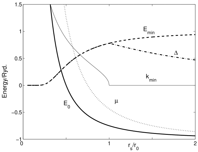
Figure 2: Sketch of the energy per particle $E_{0}$ (solid line) and chemical potential $\mu$ (dotted) relative to the band edge, along with the correlation gap $\Delta=\Delta(k_{min})$ (dash-dot). Also shown is the minimum excitation energy $E_{min}=\min(E_{k})$ (dashed) and the wavevector $k_{min}$ (think solid line) of the minimum gap. Typically, the density parameter $r_{0}$ marking the BCS-BEC crossover is around 2-3.

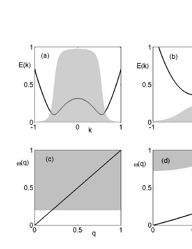
Figure 3: (a) and (b) show a sketch of the quasiparticle spectrum $E(k)$ (lines) and the occupation factor $v(k)^{2}$ (grey hatching) on either side of the BCS crossover. In the lower panels, (c) and (d) give for comparable regimes the spectrum of excitations of total momentum $q$. In the dense (BCS) limit (c) shows a steeply rising phase mode and most of the phase space is occupied by gapped particle-hole excitations. In the dilute limit (d) the particle hole spectrum is at the ionisation energy, and the phase mode provides the dominant fluctuations.

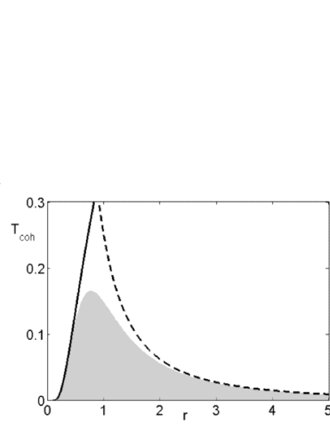
Figure 4: Estimates of the coherence temperatures in $Ryd.$ for the BCS limit (solid line, Eq. (37)) and the BEC limit (dashed line, Eq. (38)). The parameter $A=1$ and the scale for the BCS limit has been fit to the calculations of coupled quantum wells of [45], and $m_{e}=m_{h}$. The gray hatching is a smooth interpolation between the limits.

Although this seems like a sensible treatment of the ground state wavefunction and low temperature properties, it is a poor theory for finite temperature. Clearly a BCS theory of $T_{c}$ will estimate the transition temperature to be of order $E_{min}$, which is sensible at large density, but clearly nonsense in the bosonic limit. The error is well-known – the BCS excitation spectrum is missing the collective excitations. Notice that the excitations in the BCS state are all pair-breaking excitations with total momentum $q=0$. There is no sign of the sound mode expected from the Bogoliubov spectrum (24), which one would certainly expect to recover in the dilute limit. This is in fact a traditional problem with mean-field theories of correlated ground states: for example the Slater (or Hartree-Fock) theory of magnetism is missing a spin-wave spectrum; the BCS theory of superconductivity misses the Bogoliubov phase mode; the mean-field theory of charge- and spin-density waves is lacking a “phason” or sliding mode. In the present problem, notice that in the low density limit we are also apparently missing all of the bound exciton excited states, despite that the ground state wavefunction is of course exact as $r_{s}\to\infty$.

Conveniently,the problem is also straightforwardly rectified, following methods that were first developed for superconductivity [56]. One method to do this – that preserves the high energy structure (on scales of order the gap) as well as giving the appropriate low energy theory – is to go back to the complete derivation of the (single) exciton spectrum (including its centre of mass motion) by calculating the repeated interaction of an electron and a hole. This is discussed carefully by Mahan[57]. For a single exciton it gives the usual spectrum, with both the free motion of the center of mass and the series of bound excited states of higher internal quantum numbers.

In the condensed state, one should repeat this calculation but now using the quasiparticle propagators of Eq. (32). Now we find that the 1S exciton dispersion becomes linear at small $q$, which is the Bogoliubov mode we expected in analogy to Eq. (24). Detailed results have been given by Keldysh and Koslov[25], and others [58, 59]. There is an equivalent functional field theory approach to this scheme, which by explicitly preserving the gauge symmetry of the low energy theory guarantees the correct form of the phase mode [43] and runs close to the line of Section 3.2.

The algebra can become messy, but the physics in two limits is clear, and most of the useful results can just be sketched by hand. Fig. 3 contrasts the excitation spectrum in the low and high density limit. At high densities, the phase mode has a steep velocity $s$ of order the Fermi velocity $\approx v_{f}$, because the energy of a pair excitation is almost entirely the (large) kinetic energy of two fermions shifted from the Fermi surface by momentum $q$, i.e. $s\approx qd\epsilon_{k}/dk|_{k_{f}}$. The mode then runs into the continuum at a momentum of order $1/\xi_{BCS}$ with $\xi=\hbar v_{f}/\Delta$ the familiar BCS coherence length. Provided $n\xi^{d}\gg 1$, the phase space where the sound mode is of lowest energy is small, and consequently the dominant thermal excitations that destroy the superfluid order are broken pairs. In contrast, at low density, the particle hole gap is large, of order the Rydberg, while the sound velocity is approximately given by the Bogoliubov result discussed above

$$Ms^{2}\approx n_{o}V_{o}=3\frac{m}{M}\frac{a}{a_{o}}\frac{1}{r_{s}^{3}}{\rm Ry.}$$ (35)

in three dimensions. Here we have re-expressed the interaction potential between dilute excitons in terms of the scattering length via $V_{o}=4\pi\hbar^{2}a/M$, $m$ is the exciton reduced mass, and $M$ the exciton mass. (On physical grounds one expects $a\propto a_{o}$, though for long range dipole interactions between 2D excitons, this approximation may not be used.) The linear dispersion turns quadratic for momenta larger than the inverse of the healing length, which is

$$\frac{\xi}{a_{o}}=\left(\frac{r_{s}^{3}a_{o}}{6a}\right)^{1/2}.$$ (36)

So in this limit, the phase mode turns smoothly into the kinetic energy of the 1S exciton; it never intersects the continuum, instead running parallel to it. (There also exists the Rydberg series of excited states of the pairs, neglected here for simplicity.)

We can now estimate the crossover in the transition temperature from dense to dilute limits, expressed in exciton Rydbergs for convenience. In the BCS limit we will get

$$\frac{kT_{c}}{Ry.}\approx e^{-1/g}\approx e^{-A/r_{s}}\;\;\;{\rm for}\;r_{s}\ll 1,$$ (37)

where $g\approx V_{eh}(k_{f})/E_{f}\propto r_{s}$ and $A$ is a constant of order unity. In the dilute limit we shall have a transition temperature of order the degeneracy temperature in the non-interacting Bose gas

$$\frac{kT_{c}}{Ry.}\approx\frac{m}{M}\frac{1}{r_{s}^{2}}\;\;\;{\rm for}\;r_{s}\gg 1.$$ (38)

Thus $T_{c}$ is a strong function of density peaking near $r_{s}\approx 1$, and vanishing in both low and high density limits.

An estimate for bilayers is shown in Fig. 4. Since the system is two-dimensional the actual transition will be of Kosterlitz-Thouless character, and thus reduced by a numerical factor from the mean-field estimates given here. More important than the quantitative changes in $T_{c}$ is here the fact that long-range order will not occur at any non-zero temperature, because although there is the rigidity provided by the acoustic mode, thermal fluctuations of the phase mode decorrelate the phase of the order parameter. This has pronounced effects on the phase-coherent emission of light[60].

3.5 Miscellaneous remarks

We make a few small remarks and caveats about the solutions here.

Because we used a bandstructure model with isotropic dispersion, the electron and hole Fermi surfaces are always perfectly nested, and therefore even at infinite density there is a nesting instability of the Fermi seas to an excitonic insulator with a tiny gap. This is suppressed by realistic bandstructure effects – for example in GaAs the hole bands are anisotropic, being based on p-orbitals – so that there is a sharp onset of $T_{c}$ at a critical density. Once the Coulomb interaction is itself a sizeable fraction of the kinetic energy, the transition is no longer driven by a nesting instability.

The BCS wavefunction itself gives a poor bound for the overall energy of the ground state, largely because it neglects the short range correlation of like species. Improved wavefunctions of the Jastrow form[47, 48] give lower energies without destroying the qualitative description encapsulated by the BCS state. In particular, there appears to be no stable electron-hole liquid state in a direct-gap semiconductor (i.e. a minimum in the ground state energy per particle at large density, below the binding energy of exciton or biexciton), unlike the case of the indirect gap Ge[61].

Bilayers are particularly advantageous in that the dipole repulsion between individual excitons strongly disfavours biexciton formation. In order to prepare a quasi-equilibrium state of excitons not under direct illumination, it is necessary to prepare traps, perhaps by ambient disorder[62, 63], well-width fluctuations[64], or strain[65]. These all turn out to be relatively shallow, and the density distribution of excitons changes very little through the condensation transition [60]. Thus, in contrast with the cold atom systems, the direct spatial imaging of density is not expected to provide dramatic evidence for condensation.

We have ignored spin, and of course excitons made of s=1/2 fermions will come in singlet ($L=0$) and triplet ($L=1$) varieties. In GaAs and similar systems, because the (spin-orbit coupled) heavy and light hole states have $J=3/2$, there are optically active excitons with angular momentum $L=\pm 1$ as well as dark excitons with $L=\pm 2$. In quantum wells, the broken degeneracy between heavy and light hole bands yields two energetically well-separated exciton species[66]. In the bilayer quantum well systems, interband exchange is certainly much too small to give significant energetic splitting between spin species, thus if equilibrium is established between the spin species the only effect is to replace $r_{s}\to g^{1/2}r_{s}$, with $g$ the spin degeneracy[26, 64].

We stress again the neglect of tunnelling and recombination. There are systems of type II heterostructures (e.g. InAs/GaSb) where the conduction band of one material lies below the valence band of the other. Thus an interface between the two will produce a pair of inversion layers (electrons and holes) in close proximity. Generally, the overlap between electron and hole will not be negligible, so that tunnelling terms $tc^{\dagger}v$ will exist in the Hamiltonian, and exciton conservation is destroyed. Firstly, this will introduce a gap in the spectrum even without Coulomb correlation (the system may become an insulator or semimetal)[67]. More generally, the gauge symmetry is broken so that the order parameter $<c^{\dagger}v>$ has its phase fixed by the tunnelling matrix element, and the Bogoliubov mode has a gap. Only should the tunnelling be vanishingly small (as it may be in the quantum Hall bilayer systems [39, 40]) can one expect to approach superfluid behaviour.

4 Theory of polariton condensation

Excitons are of course excitations above the ground state – so in order to work with an out-of-equilibrium ensemble in the previous section we introduced a chemical potential and enforced thermal equlibrium. But in many semiconductors, there is a direct recombination channel of excitons into dipole radiation, which is suppressed but not eliminated, for example, in the bilayer systems, because recombination requires tunnelling between the coupled quantum wells.

The decay of excitons into photons can of course provide evidence for the coherence in the exciton system, both temporal[62, 70] and spatial[60]. If the coupling is weak, as in the coupled quantum wells, or in $\mathrm{Cu_{2}O}$, then the exciton system is only lightly perturbed by the decay process. However, there is a different limit of strong coupling that can be obtained by exciting excitons inside optical microcavities[17]. If the photons are well-confined by mirrors, then the appropriate linear excitation is a superposition of photon and exciton, called a polariton[18]. This is a new type of boson, and on account of its light mass, seems a natural candidate for polaritonic BEC[6, 68, 69] at substantial temperatures. Of course, since photons are not conserved, we must again consider the quasi-equilibrium situation of a pumped system with (nearly perfect) mirrors that has attained thermal equilibrium with a bath that establishes a chemical potential for the excitation number.

Free photons in the cavity are described by the microscopic quasi two-dimensional Hamiltonian

$$H_{\mathrm{ph}}=\sum_{{\bf p}}\psi_{{\bf p}}^{\dagger}\left[\omega({\bf p})-\mu\right]\psi_{{\bf p}}\;,$$ (39)

where their dispersion, $\omega({\bf p})=\sqrt{\omega_{c}^{2}+(c{\bf p})^{2}}$, is quantised in the direction perpendicular to the plane of the cavity mirrors, and we shall just keep a single branch of the cavity modes, beginning at $\omega_{c}=c\pi/L$ (whose value is fixed by the cavity thickness $L$).

In the dipole and rotating-wave approximation, the photons are assumed to be coupled to the electron-hole system through a local interaction,

$$H_{\mathrm{dip}}=g\int d{{\bf r}}\left[\psi({\bf r})a_{c}^{\dagger}({\bf r})a_{v}({\bf r})+\mathrm{h.c.}\right].$$ (40)

In practice, one chooses $\omega_{c}$ to be close to the exciton frequency so the resonant coupling dominates. Since we are dealing with a system where the physical temperature is much smaller than the photon frequency $\omega_{c}$, we may neglect the tiny spontaneous population that would be generated by non-resonant terms. To mimic the effect of the external excitation source, we suppose that the electron-hole/photon system is held in quasi-equilibrium by tuning the chemical potential $\mu$ in Eq. (28) to fix the total number of excitations

$$\hat{N}_{\mathrm{ex}}=\sum_{{\bf p}}\psi^{\dagger}_{{\bf p}}\psi_{{\bf p}}+\frac{1}{2}\sum_{{\bf k}}\left(a_{c,k}^{\dagger}a_{c,k}-a^{\dagger}_{v,k}a_{v,k}+1\right)\;.$$ (41)

However, how the system chooses to portion the excitations between the electron-hole and photon degrees of freedom depends sensitively on the properties of the condensate.

In the previous sections, we were at pains to stress the difference between the statistical physics of BEC of non-interacting bosons, and the phase transition accompanying coherence. A single polariton is a phase-coherent object, delocalised over the whole system and producing a coupled oscillation in the electric displacement field ${\bf D}$ (of light) and the excitonic polarisation ${\bf P}$. Polariton condensation would lead to a macroscopic coherent optical field in the cavity (phase-locking of the polariton modes), and hence bear considerable similarity to a laser[6, 70]. What is special about the condensed polariton state is that the excitonic component is also coherent, whereas this is strongly dephased in a conventional laser, and only a coherent photon field exists.

For strongly detuned excitons and photons, exciton-photon condensation can be described either in terms of polariton condensation or as exciton condensation with both the Coulomb interaction and a photon-mediated interaction. If the excitons are localised, we expect the photon-mediated interaction to dominate, because its range is usually larger than that of the Coulomb interaction between excitons.

4.1 Mean-field wavefunction

There is now a very natural extension of the Keldysh mean field wavefunction to propose for the coupled problem, viz.

$$|\Psi_{0}>=e^{\lambda\psi_{0}^{\dagger}}\prod_{\vec{k}}[u_{\vec{k}}+v_{\vec{k}}a_{c,k}^{\dagger}a_{v,k}]|0\rangle.$$ (42)

Now one has, in addition to the variational functions $u,v$, a variational parameter $\lambda$. This is a state which is a coherent state of photons (in the lowest mode of the cavity), and a coherent state of excitons. The equations which arise from a variational minimisation of $\langle\Psi_{0}|H|\Psi_{0}\rangle$ couple these order parameters, and the relative proportions of photon and exciton in the ground state depend on details such as the relative tuning of the exciton and photon energy; but both take macroscopic values in the state $|\Psi_{0}\rangle$ of Eq. (42).

The variational equations can be found elsewhere[43], and we will here just discuss the results qualitatively. Just as the Keldysh wavefunction, Eq. (27), approximates a condensation of structureless excitons in the low-density limit ($v\ll 1$), in the same limit Eq. (42) will look like a Bose condensate of polaritons. In the dense limit, $v_{k}$ approximates a Fermi function and only close to the chemical potential is there any renormalisation of the spectrum. If one detunes the photon frequency far from the chemical potential (i.e. $|\omega_{c}-\mu|\gg g\lambda$) the results are barely changed from the old mean field theory because the interaction is dominated by direct Coulomb forces; but in the opposite limit,

$$\frac{g^{2}}{|\omega_{c}-\mu|}\gg Ry^{*},$$ (43)

the Coulomb interaction is not the relevant source of pairing, instead it is the photon field itself.

As far as the electronic excitations which form the condensate are concerned, they are then identical to those predicted by the well-known Hartree-Fock theory of a semiconductor in an external classical time-dependent field[71, 72]. The most obvious difference from the driven problem is just that the photon field has to be established self-consistently, but this is just a (complex) technical matter. A more hidden (and more important difference for the robustness of the state) is that the excitation spectrum for the quasi-electron and quasi-hole is occupied according to equilibrium (fermionic) statistics.

4.2 Localised exciton model

A simplified model that replaces the excitons by localised two-level systems is a good way to exhibit the physics in the photon dominated regime.

The model is the Dicke model of atomic physics[74]:

$$H_{2level}=\sum_{\bf q}\omega({\bf q})\psi_{{\bf q}}^{\dagger}\psi_{{\bf q}}+\sum_{j=1}^{N}\frac{\epsilon_{j}}{2}(b^{\dagger}_{j}b_{j}-a^{\dagger}_{j}a_{j})+\frac{g}{\sqrt{N}}\sum_{j{\bf q}}(b^{\dagger}_{j}a_{j}\psi_{{\bf q}}+\psi^{\dagger}_{{\bf q}}a^{\dagger}_{j}b_{j})\;\;.$$ (44)

$H_{2level}$ describes an ensemble of N two-level oscillators with an energy $\epsilon_{j}$ dipole coupled to one cavity mode. $b$ and $a$ are fermionic annihilation operators for an electron in an upper and lower states respectively (with a local constraint $b_{j}^{\dagger}b_{j}+a_{j}^{\dagger}a_{j}=1$ so that there is an electron either in the lower level or in the upper level) and $\psi$ is a photon bosonic annihilation operator. The operator that counts the number of excitations in the system, $N_{ex}=\sum_{q}\psi_{{\bf q}}^{\dagger}\psi_{{\bf q}}+\frac{1}{2}\sum_{j}(b^{\dagger}_{j}b_{j}-a^{\dagger}_{j}a_{j}+1)$, commutes with $H_{2level}$ so is conserved.

The mean field wavefunction is then

$$|\lambda,u,v\rangle=e^{\lambda\psi_{0}^{\dagger}}\prod_{j}(v_{j}b_{j}^{\dagger}+u_{j}a_{j}^{\dagger})|0\rangle.$$ (45)

with the (real) variational parameter $\lambda$ and variational functions $v_{j}=v(\epsilon_{j})$. (The vacuum state is here defined to be empty of both levels.) The constraint is satified by setting $u_{j}^{2}+v_{j}^{2}=1$, and the variational functions are obtained by minimising $H_{2level}-\mu N_{ex}$. For detailed results see [31, 32]. Notice that this approximation neglects coupling to all but the ${{\bf q}}=0$ photon mode at $\omega_{c}$.

To connect to the earlier theory of pure fermions, consider the case when $\delta=(\omega_{c}-\epsilon)/g\gg 1$. Now provided the occupation is fairly small (less than or order of 1 per site), the chemical potential will lie in the band of two level systems, the photon occupation will be small, and the photons will act to provide a virtual interaction between the excitons of magnitude $g_{eff}=g^{2}/(\omega_{c}-\mu)$.

The results are most easily visualised with a distribution of energies, and in Fig. 5 are shown the occupancies calculated for a gaussian distribution of energy levels, as the excitation level $\rho_{x}=N_{ex}/N$ is increased. Notice that at low densities, the distribution approaches the step function of a Fermi distribution, and becomes broadened as the density increases, counter to the results of the Coulomb problem in Fig. 1. The reason is that the gap in the two-level model is not fixed but is provided by the photon field, whose amplitude is growing with $\rho_{x}$; for $\rho_{x}>1$ the order parameter becomes increasingly photon-like. In fact as $\rho_{x}\to\infty$, then $v^{2}\to\frac{1}{2}$ — the system saturates with the two-level distribution held just above the border of inversion. When the photon and exciton are detuned from each other (as in the case shown in the figure) this evolution is not monotonic, because the chemical potential jumps discontinuously from being within the band of two level systems to be close to the photon.

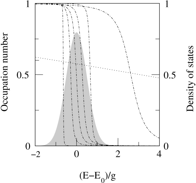
Figure 5: Occupancy $v(\epsilon)$ as a function of two level system energy $\epsilon$ where the photon energy is substantially detuned (above) the centroid of the exciton distribution ($\omega_{c}-<\epsilon>=3g$). The different curves correspond to $\rho_{x}=0.1,0.3,0.5,0.7,0.9$ (dot-dash increasing from left to right) and $\rho_{x}=101$ (dotted curve). The grey hatching is the density of states $\nu(\epsilon)$ of the two-level systems. From [32].

Just as in the exciton case, we can extend the mean-field theory to finite temperatures by solving the self-consistent equations assuming a thermal occupancy of quasiparticles, as in BCS theory. The transition temperature is determined by setting $\lambda=0$ in the BCS-like gap equation

$$\frac{1}{g_{eff}}=\int\frac{\tanh(\frac{\beta E(\epsilon)}{2})}{E(\epsilon)}\nu(\epsilon)d\epsilon$$ (46)

$$E(\epsilon)=\sqrt{(\epsilon-\mu)^{2}+4|\lambda|^{2}},$$ (47)

where $\nu(\epsilon)$ is the density of states of the two-level oscillators. If $\mu$ lies in the band of two-level oscillators then at low temperatures(relative to the bandwidth of these oscillators), the integral on the right of (46) is approximately $-2\nu(\mu)\ln(\beta\theta)$, where $\theta$ is a cut-off associated with the bandwidth of the oscillators. This gives us an approximate expression for the transition temperature

$$\ln{\frac{kT_{mf}}{\theta}}\approx\frac{-1}{2g_{eff}\nu(\mu)},$$ (48)

valid when the computed $T_{mf}$ is small compared with the bandwidth $\theta$. If instead the temperature is large compared with the bandwidth, we can express the transition temperature in terms of the dimensionless detuning $\delta=(\omega_{c}-\epsilon)/g$, the density $\rho_{x}$, and the coupling g as

$$kT_{mf}=gf(\rho_{x},\delta)=g\frac{\delta\pm\sqrt{\delta^{2}-8\rho_{x}+4}}{4\tanh^{-1}(2\rho_{x}-1)}.$$ (49)

The normal state of this model is an incoherent population of excitons. The phase transition occurs when the chemical potential for the excitons crosses the energy of a coupled exciton-photon mode of zero wavevector. At low densities, the energy of the lowest coupled exciton-photon state is just that of the conventional, linear response polariton $E_{LPB}$, and the two-level systems are occupied according to a Boltzmann distribution. Thus the critical density should be $\rho_{x}=e^{-\beta(\epsilon-\mu_{c})}=e^{-\beta(\epsilon-E_{LPB})}$, which is indeed the low-density limit of (49). At higher densities the form changes, because the occupation of two-level systems is no longer a Boltzmann factor, and because the energy of the coupled exciton-photon mode is renormalised by the occupation of the two-level systems.

There are some unusual features of the phase diagram of this model that are produced by the saturable nature of the excitons. One of these is the multivalued phase boundary (49), whose two values correspond to the chemical potential crossing either of the two coupled exciton-photon modes of zero wavevector. One might expect the higher energy crossing to be irrelevant, as the system would already have condensed before it is reached. This is not necessarily true, however, because the exciton entropy decreases with increasing density when $\rho_{x}>0.5$. Thus, at high enough temperatures, the system can be stable against an excitation which increases the density, even if it decreases the energy. In the region where the normal-state entropy decreases with increasing density, $0.5<\rho_{x}<1$, we find that the normal state is stable if its chemical potential lies above the lower polariton and below the upper polariton. Another peculiarity is that for $\rho_{x}>1$ the saturation forces some of the excitation into the photon, so the system is condensed at any temperature.

We now discuss the general behaviour of the transition temperature in the case of a finite bandwidth and a cavity mode lying well above the band. At low densities the chemical potential will lie towards the bottom of the band, $g_{eff}$ will be small, and if the band is broad enough the weak-coupling form (48) will apply. As we increase the density the chemical potential rises, and the transition temperature increases exponentially as the density of states and $g_{eff}$ increases. If the band is broad and the detuning large enough, the weak-coupling form would continue to hold right through the band. After $\mu$ has moved through the centre of the band the density of states begins to decrease, and this could produce a decrease in $T_{mf}$, although it could be offset by the increasing $g_{eff}$. As the density is further increased towards $\rho_{x}=1$, the weak-coupling form breaks down as $\mu$ moves into the upper tail of the band. The chemical potential rapidly jumps up to near the photon frequency, and the transition temperature diverges according to the strong-coupling form (49).

The weak-coupling scenario bears some comparison to the high-density Coulomb coupled exciton condensate, because in both cases the effective interaction is small compared with the bandwidth. The differences arise because $g_{eff}$ increases with increasing density, and because the density-of-states is a function of density. Thus while in the Coulomb-coupled condensate the transition temperature either saturates or decreases with increasing density, depending on whether we include screening or not, here we find more complicated behaviour.

Let us describe two other scenarios for $T_{mf}$. Suppose first that we keep the photon above the band, but reduce the detuning or bandwidth. Then there will be a region of density where the weak-coupling form fails, and we need either the strong-coupling form (49) or the full solution to the gap equation (46). Or consider the case when the photon is below the peak of a broad band. Then as the density increases the transition temperature simply crosses from the weak- to strong- coupling forms, diverging as $\mu\to\omega_{c}$.

While in the Coulomb problem the mean-field theory is only expected to hold in the weak-coupling limit, we expect the mean-field theory of polariton condensation in systems with localised excitons to be more generally valid. This is because the photons provide a long-range interaction between the excitons, so we expect mean-field theory to be a good approximation. It is interesting to note that while the mean-field theory is an approximate theory for the extended system, for a model which has only a single photon mode (i.e. a zero-dimensional microcavity), it becomes exact in the thermodynamic limit ($N\to\infty$; $\rho_{x}\to{\mathrm{c}onst.}>0$)[32]. There has been progress on solving that model at finite $N$[75].

4.3 BEC to polariton laser to BCS crossovers

Because we worked with only a single mode of the electromagnetic field, our discussion of polariton condensation makes no mention of the polariton effective mass. The theories of polariton condensation we have discussed have the character of BCS theory, in that finite temperatures destroy the order by creating excitations across the gap. In the two-level model this gap, which plays the role of the superconducting gap $\Delta$ in BCS theory, is $g<\psi>$, whereas in the electron-hole model the gap will involve both the optically-mediated interaction $g$ and the Coulomb interaction. Either way, the transition temperature in these theories is determined by an interaction strength, and not by an effective mass as it would be were we to regard the polaritons as structureless, weakly-interacting bosons. In that theory, we would expect the onset of coherence at a temperature

$$k_{B}T_{BEC}\approx\frac{\hbar^{2}\rho_{x}}{2M^{*}}=\frac{\hbar c^{2}\rho_{x}}{4\omega_{c}},$$ (50)

where we have substituted for the polariton mass $M^{*}=2\hbar\omega_{c}/c^{2}$ in the case of resonance, i.e. $\omega_{c}=\epsilon$. This temperature increases rapidly with density since the polariton has a very light mass: $M^{*}/m=2\hbar\omega_{c}/(mc^{2})\approx 10^{-5}$. But of course it then rapidly reaches a scale of order $g$ when the dominant fluctuations are not the long-wavelength phase modes, but excitations across the gap. To estimate where the crossover occurs, we introduce the dimensionless density in the usual fashion $\pi r_{s}^{2}a_{*}^{2}=1/\rho_{x}$ so that we can rewrite Eq. (50) as

$$\frac{k_{B}T_{BEC}}{g}\approx\frac{Ry^{\ast}}{g}\frac{m}{M^{*}}\frac{1}{2\pi r_{s}^{2}}.$$ (51)

Thus polariton BEC in the conventional sense is expected to be the appropriate theory only for $r_{s}>100/(g/Ry)^{1/2}$; the promising experimental systems all have coupling constants no more than a few $Ry.$ and so the regime of applicability is small indeed. At higher excitation levels the relevant theory is then the mean field theory of the last section. These estimates for the crossover differ somewhat from those made in [68].

Of course, as we saw in the last section, once the system reaches substantial photon densities (approaching the conventional inversion point for the laser), the mean-field theory gives an unphysical infinite transition temperature. This implies that there must then be a second crossover back to a regime where fluctuations into states of finite momentum are important. Because lower branch polaritons at large momentum (outside the light cone) are essentially excitons uncoupled to the photon bath, this reservoir has a very large density of states that depletes the condensate and reduces the transition temperature[33].

We now see that there is typically a substantial regime where may find a polariton condensate in the strong coupling regime but where $r_{s}\gg 1$; here our approximation of replacing mobile excitons by localised two-level systems can be a good one. Yet if $r_{s}$ is small enough (or at least that part of the density that is excitonic in character) we will have to deal with a realistic model of exciton unbinding - the Coulomb interaction will play a role. This will produce a second crossover akin to that discussed in Sec. 3.4. Nevertheless, even here there will be a regime where the photon field will dominate the Coulomb interaction, to be reached at high excitation levels[43].

Figure 6 provides a rough and ready estimate of the various regimes that may appear for delocalised excitons together with the coupling to photons in a microcavity. The vertical axis is the direction of the conventional BCS-BEC crossover of Sec. 3.4. However, if there is coupling mediated by photons, this will always dominate in the model both at very low density and very high density — the photon-mediated coupling is finite and long range, whereas the direct Coulomb coupling is irrelevant in the two extreme limits. Of course in the physical system, one cannot tune independently the photon density and the exciton density, because these adjust their balance to maintain a common chemical potential.

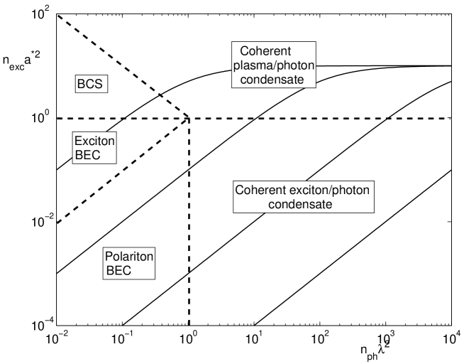
Figure 6: Sketch to demonstrate the various crossovers in the polariton problem. The dimensionless densities are plotted on the two axes $n_{exc}a^{*2}$ for excitons and $n_{ph}\lambda^{2}=n_{ph}\hbar^{2}/2M^{*}g$ for photons. The crossover from BEC of polaritons to an interaction-driven polariton condensate occurs when $n_{ph}\lambda^{2}\approx 1$; the conventional BEC/BCS crossover for excitons occurs when $n_{exc}a^{*2}\approx 1$, and at large photon numbers this marks the conventional point of inversion for a plasma “laser”. The two wedges labelled BCS and exciton BEC consitute the regime where the Coulomb interaction is the dominant coupling term. The solid lines are rough guides to trajectories that would be followed for a fixed ratio of the coupling constants $(a^{*}/\lambda)^{2}=(g/Ryd.)(M^{*}/m)=10,\;10^{-1},\;10^{-3},\;10^{-5}$. In order for the electron-hole density to be able to reach such high values as shown, the cavity mode frequency would need to be placed well above the edge of the band.

4.4 Decoherence and disorder

Is indeed the polariton condensate just a laser? In fact it differs very much from the conventional textbook description, which has a coherent optical field (ignoring finite size fluctuation effects) but is not generally thought to have a coherent internal polarisation. The usual assumption of laser physics is that the electronic polarisation is described by a Langevin equation with a short decoherence time[76]. There is also a distinction to be made between most solid state lasers where the electronic excitations are localised (usually atomic in nature, and thus describable as localised excitons) and GaAs semiconductor lasers that are usually operated in a regime where the excitons are unbound (corresponding to a hot two-component plasma)[77, 78]. But notice that the latter distinction is quite independent of whether or not the electronic polarisation has a short decoherence time – in principle either a plasma or an array of two-level systems can support a coherent polarisation.

The origin of decoherence is elastic and inelastic scattering whereby the fundamental excitations are coupled to continuum degrees of freedom in an open system. There are many sources of decoherence: Because the mirrors are not perfect, light will leak out of the lasing mode and the excitation (in steady state) must be replaced by incoherent pumping of excitons; Excitons themselves may decay spontaneously into photon modes other than the cavity mode; Phonons and disorder inside the material can scatter the excitons, and produce pairbreaking and dephasing. All of these may be modelled by coupling of the internal degrees of freedom to (bosonic) baths of dynamic fluctuations $B_{\gamma}({\bf r},t)$. If we consider the Dicke model (44), but relax the local single occupancy constraints $b_{j}^{\dagger}b_{j}+a_{j}^{\dagger}a_{j}=1$, then these fluctuations will be of three generic types:

$$H_{SB} = \sum_{j=1}^{N}(b^{\dagger}_{j}b_{j}-a^{\dagger}_{j}a_{j})(B_{1j}^{\dagger}+B_{1j})+$$ (52)

$$+ \sum_{j=1}^{N}(b^{\dagger}_{j}b_{j}+a^{\dagger}_{j}a_{j})(B_{2j}^{\dagger}+B_{2j})+$$

$$+ \sum_{j{\bf q}}(b^{\dagger}_{j}a_{j}B_{3j}^{\dagger}+a^{\dagger}_{j}b_{j}B_{3j}).$$

This is already a simplification in that we have kept just diagonal terms. The three terms in Eq. (52) correspond to neutral, pairbreaking, and phase-breaking scattering respectively. Their treatment in a quasi-equilibrium situation is discussed in [41, 42].

The first term in Eq. (52) represents dynamic or static fluctuations of the excitation energy $\epsilon_{j}$. Provided these fluctuations are slow and weak enough, they are relatively harmless to the ground state: the wavefunction is robust against static disorder in the energy levels, in a similar way that a singlet superconductor is insensitive to weak charge disorder.

The second term is more dangerous, and if a static potential plays just the same role as magnetic impurities in a superconductor[79, 80]. This corresponds to scattering that breaks up the electron-hole pair (in order for it to be relevant, one must relax the two-level constraint). At the mean field level, this leads first to a reduction in the gap, and then to a gapless excitation spectrum that is still phase coherent. If one is at excitation levels $\rho_{x}<1/2$, then with increasing disorder the coherent state is suppressed. But at larger excitation levels $\rho_{x}>1/2$, the coherent state remains: with increasing disorder the order parameter becomes dominated by the light field, the excitation spectrum becomes uniform, and the coherent electronic polarisation is continuously reduced to very small values. Such a gapless condensate reproduces the conventional semiconductor laser as an incoherent electron-hole system, with no bound excitons. But this is a very different state than we would have got if we had modelled a high density electron-hole system with Eq. (42) — such a state has a gap in the spectrum (for example, the region labelled as a “interacting polariton condensate” in Fig. 6). One can add pairbreaking scattering to such a state to explore the close formal analogy with a superconductor, though the two-component light-supported order parameter again generates new physical regimes[43]. But all in all, incoherent pair-breaking and high electron-hole densities (which tend to go together) drive one into the conventional laser regime. Strong pair-breaking destroys entirely the “interacting polariton condensate” regime of Fig. 6.

The last term in Eq. (52) does not exist in a superconductor where it would be forbidden by symmetry. This is an XY-like random-field term (coupling to $S_{x}$, $S_{y}$ if we represent two-level systems as a spin model); it is sensitive to the phase of the local order parameter. Such a term will formally destroy the long-range order of the condensate even if infinitesimal (in dimensions below 4) — but since we have a system with long-range coupling via the optical field, many physical effects of the ground state will remain in the limit of large system size. The role of this term is presumably to suppress the quantum fluctuations in a finite system, and to lead to slow diffusive dynamics of the semiclassical order parameter. But it has not yet been studied carefully. Certainly when this term is large enough, it will be expected to lead us toward the conventional solid state laser model of localised excitations but with rapid dephasing. For small systems, this leads us toward the regime of the “few-atom laser”[81], but potentially in the strong coupling regime of large entanglement.

In most practical situations, the effects of scattering and decoherence will strongly suppress the coherent phases appearing at high pumping levels in Fig. 6, and replace them with more conventional weak coupling lasers. Some recent experiments have however demonstrated spontaneous coherence in the regime that can be termed a polariton laser[22].

5 Conclusions

This review has attempted to link the central idea of coherence across the very different physical systems of a dilute Bose gas, excitons, and polaritons. Using a microscopic model of a coherent state wavefunction, and the macroscopic consequence of phase coherence, the many parallels between these systems - and that of superconductivity - are exposed. Furthermore, by understanding the effects of static or dynamic symmetry breaking fields, we can provide a theoretical framework to connect to the classical regime of the laser.

There are many things left out. Because our concern has been with the structure of the theory, we have not discussed experimental systems and experiments except superficially. Nor have we discussed at any length the physical consequences of condensation and hence the critical experimental tests – though some of these are implicit.

We have also addressed only thermal equilibrium. Dealing with strongly driven systems that are far from thermal equilibrium is an interesting and difficult challenge that is worth extended theoretical effort. One of the interesting features of the experimental systems is that they are routinely driven very far from equilibrium, into regimes that are impossible to reach in conventional solids. There are many avenues that are yet to be addressed: Can one maintain coherence in a pumped - but perhaps steady state - system? What is the temporal evolution as condensation develops? Non-equilibrium methods using Langevin dynamics, and the language of stimulated scattering, are well developed in the laser arena, and those ideas have been applied to polaritons (see e.g. [69]) but it is not known what replaces this approach in the coherent case - as we argued above and elsewhere[42] the Langevin equation has no place when phase coherence is dominant.

We have focussed on bulk systems, and in the case of the polariton condensate, nearly mean-field-like systems. For example, the cold fermion systems coupled via a Feshbach resonance have a formally similar theory[37] to polaritons to describe them, but however with a mediating boson - in this case a molecule - that is much smaller than the characteristic separation between fermions. Also the polariton systems are not unconfined (though driven inhomogeneously), but nevertheless have spatial structure that is currently unexplained[23]. A further exciting direction is to small systems with few photons, where the quantum statistics can be exposed. Again this is a regime that is hard to reach in conventional solids, but is quite evident in optics.

References

References

- [1] Moskalenko S A 1962 Fiz. Tverd. Tela 4 276 [1962 Sov. Phys. Solid State 4 199]
- [2] Blatt J, Brandt W and Boer K 1962 Phys. Rev. 126 1691
- [3] Keldysh L V and Kopaev Y V 1964 Fiz. Tverd. Tela 6 2791 [1965 Sov. Phys. Solid State 6 2219]
- [4] 1994 Bose-Einstein Condensation ed A Griffin et al (Cambridge: Cambridge University Press)
- [5] Moskalenko S A and Snoke D W 2000 Bose-Einstein Condensation of Excitons and Biexcitons and Coherent Nonlinear Optics with Excitons (Cambridge: Cambridge University Press)
- [6] Hanamura E and Haug H 1977 Physics Reports 33 209
- [7] Wolfe J P, Lin J L, Snoke D W in [4] p 281
- [8] [] O’Hara K E, Suilleabhain L O and Wolfe J P 1999 Phys. Rev. B 60 10565
- [9] Kuwata-Gonokami M, Shimano R and Mysyrowicz A 2002 J. Phys. Soc. Japan 71 1257
- [10] Lozovik Y E and Yudson V I 1975 Pis’ma Zh. Eksp. Teor. Fiz. 22 556 [1975 JETP Lett. 22 274]
- [11] [] Shevchenko S I 1976 Fiz. Nizk. Temp. 2 505 [1976 Sov. J. Low Temp. Phys. 2]
- [12] Kash J A, Zachau M, Mendez E E, Hong J M and Fukuzawa T 1991 Phys. Rev. Lett. 66 2247
- [13] [] Kash J A, Zachau M, Mendez E E, Hong J M and Fukuzawa T 1992 Phys. Rev. Lett. 69 994
- [14] Butov L V, Lai C W, Ivanov A L, Gossard A C and Chemla D S 2002 Nature 417 47
- [15] Butov L V, Gossard A C, and Chemla D S 2003 Nature 418 751
- [16] Snoke D W, Denev S, Liu Y, Pfeiffer L, and West K 2003 Nature 418 754
- [17] Weisbuch C, Nishioka M, Ishikawa A, and Arakawa Y 1992 Phys. Rev. Lett. 69 3314
- [18] Hopfield J J 1958 Phys. Rev. 112 1555
- [19] Dang L S, Heger D, André R, Boeuf F and Romestain R 1998 Phys. Rev. Lett. 81 3920
- [20] Savvidis P G, Baumberg J J, Stevenson R M, Skolnick M S, Whittaker D M and Roberts J S 2000 Phys.Rev.Lett. 84 1547
- [21] Baumberg J J, Savvidis P G, Stevenson R M, Tartakovskii A I, Skolnick M S, Whittaker D M and Roberts J S 2000 Phys. Rev. B 62 R16247
- [22] Deng H, Weihs G, Santori C, Bloch J, and Yamamoto Y 2002 Science 298 199
- [23] Deng H, Weihs G, Snoke D, Bloch J, and Yamamoto Y, 2003 PNAS 100 15318
- [24] Weihs G, Deng H, Huang R, Sugita M, Tassone F, and Yamamoto Y 2003 Semicond. Sci. Technol. 18 S386
- [25] Keldysh L V and Kozlov A N 1968 Zh. Eksp. Teor. Fiz. 54 978 [1968 Sov. Phys.– JETP 27 521]
- [26] Comte C and Nozières P 1982 J. Phys. (Paris) 43 1069
- [27] [] Nozières P and Comte C 1982 J. Phys. (Paris) 43 1083
- [28] [] Nozières P 1983 Physica 117B/118B 16
- [29] Nozières P and Schmitt-Rink S 1985 J. Low Temp. Phys. 59 195
- [30] Randeria M in [4] p 355
- [31] Eastham P R and Littlewood P B 2000 Solid State Commun. 116 357
- [32] Eastham P R and Littlewood P B 2001 Phys. Rev. B 64 235101
- [33] Keeling J M J, Eastham P R, Szymanska M H and Littlewood P B, unpublished
- [34] Eastham P R, Szymanska M H, and Littlewood P B 2003 Solid State Commun. 127 117
- [35] Barbara P, Cawthorne A B, Shitov S V, and Lobb C J 1999 Phys. Rev. Lett. 82 1963
- [36] Harbaugh J K and Stroud D 2000 Phys. Rev. B 61 14765
- [37] Timmermans E, Furuya K, Milonni P W and Kerman A K 2001 Phys. Lett. A 285 228
- [38] Holland M, Kokkelmans S J J M F, Chiofalo M L and Walser R 2001 Phys. Rev. Lett. 87 120406
- [39] Spielman I B, Eisenstein J P, Pfeiffer L N, and West K W, Phys. Rev. Lett. 84 5808
- [40] MacDonald A H, Burkov A A, Joglekar Y N and Rossi E 2003 Physics of Semiconductors 2002, IOP Conference Series 171 p 29 (IOP Publishing) Preprint cond-mat/0310740
- [41] Szymanska M H and Littlewood P B 2002 Solid State Commun. 124 103
- [42] Szymanska M H, Littlewood P B and Simons B D 2003 Phys. Rev. A 68 13818
- [43] Marchetti F M, Simons B D, and Littlewood P B 2004 Preprint cond-mat/0405259
- [44] Guseinov R R and Keldysh L V 1972 Zh. Eksp. Teor. Fiz. 63 2255 [1973 Sov. Phys.– JETP 36 1193]
- [45] Littlewood P B and Zhu X J 1996 Physica Scripta T68 56
- [46] Littlewood P B, Brown G J, Eastham P R and Szymanska M H 2002 Phys. Status Solidi B 234 36
- [47] Zhu X J, Hybertsen M S, and Littlewood P B, 1996 Phys. Rev. B 54 13575
- [48] De Palo S, Rapisada F, and Senatore G 2002 Preprint cond-mat/0201414
- [49] Shumway J and Ceperley D M 1999 Int. Conf. on Strongly Coupled Coulomb Systems (Saint-Malo, France) Preprint cond-mat/9909434
- [50] [] Shumway J and Ceperley D M 2001 Phys. Rev. B 63 165209
- [51] Pethick C J and Smith H 2002 Bose-Einstein Condensation in Dilute Gases (Cambridge: Cambridge University Press)
- [52] Anderson P W 1966 Rev. Mod. Phys. 38 298
- [53] Nozières P in [4] p 15
- [54] Huang K in [4] p 31
- [55] Stoof H T C 2001 in Coherent Atomic Matter Waves ed R Kaiser et al (Berlin: Springer)
- [56] Schrieffer J R 1964 Theory of Superconductivity (New York: Addison-Wesley)
- [57] Mahan G D 1981 Many Particle Physics (New York: Plenum)
- [58] Côté R and Griffin A 1988 Phys. Rev. B 37 4539
- [59] Bauer G E W 1989 Phys. Rev. Lett. 64 60
- [60] Keeling J, Levitov L and Littlewood P B 2004 Phys. Rev. Lett. 92 176402
- [61] 1983 Electron-hole Droplets in Semiconductors ed C D Jeffries and L V Keldysh (New York: Elsevier)
- [62] Butov L V, Zrenner A, Abstreiter G, Böhm G, Weimann G 1994 Phys. Rev. Lett. 73 304
- [63] Larionov A V, Timofeev V B, Ni P A, Dubonos S V, Hvam I, Soerensen K 2002 JETP Lett. 75 570
- [64] Zhu X J, Littlewood P B, Hybertsen M S and Rice T M 1995 Phys. Rev. Lett. 74 1633
- [65] Negoita V, Snoke D W and Eberl K 1999 Phys. Rev. B 60 2661
- [66] Chuang S L 1995 Physics of optoelectronic devices (New York: Wiley)
- [67] Lakrimi M, Khym S, Nicholas R J, Symons D M, Peeters S M, Mason N J and Walker P J 1997 Phys. Rev. Lett. 79 3034
- [68] Zamfirescu M, Kavokin A, Gil B, Malpuech G and Kaliteevski M 2002 Phys. Rev. B 65 161205
- [69] Rubo Y G, Laussy F P, Malpuech G, Kavokin A and Bigenwald P 2003 Phys. Rev. Lett. 91 156403
- [70] Elesin V F and Kopaev Y V 1976 Pism’a Zh. Eksp. Teor. Fiz. 24 78 [1976 JETP Lett. 24 66]
- [71] Galitskii V M, Goreslavskii S P and Elesin V F 1969 Zh. Eksp. Teor. Fiz. 57 207 [1970 Sov. Phys.– JETP 30 117]
- [72] Schmitt-Rink S and Chemla D S 1986 Phys. Rev. Lett. 57 2752
- [73] [] Schmitt-Rink S, Chemla D S and Haug H 1988 Phys. Rev. B 37 941
- [74] Dicke R H 1954 Phys. Rev. 93 99
- [75] Vadeiko I P, Miroshnichenko G P, Rybin A V and Timonen J 2003 Phys. Rev. A 67 053808
- [76] Scully M O and Zubairy M S 1997 Quantum Optics (Cambridge: Cambridge University Press)
- [77] Agrawal G P and Dutta N K 1993 Semiconductor Lasers, 2nd ed (New York: Van Nostrand Reinhold)
- [78] Haug H and Koch S W 1993 Quantum Theory of the Optical and Electronic Properties of Semiconductors, 2nd ed (Singapore: World Scientific)
- [79] Abrikosov A A, Gor’kov L P 1960 J. Exptl. Theoret. Phys. (U.S.S.R) 39 1781 [1961 Sov. Phys.– JETP 12 1243]
- [80] Zittartz J 1967 Phys. Rev. 164 575
- [81] McKeever J, Boca A, Boozer J D, Buck J R, and Kimble H J 2003 Nature 425 268