Spin accumulation in ferromagnets

Abstract

Using a density matrix formulation for the effective action, we obtain a set of macroscopic equations that describe the spin accumulation in a non-homogeneous ferromagnet. We give a new expression for the spin current which extends previous work by taking into account the symmetry of the ferromagnetic state through a careful treatment of the exchange term between the conduction electrons and the magnetization, i.e., d-electrons. We consider a simple application which has been discussed previously and show that in this case spin accumulation is an interface effect confirming earlier results arrived at by different methods.

Spin-momentum transfer (SMT), was predicted by Berger Berger and Slonczewski Slon and observed experimentally Cornell ; Zurich and studied theoretically by various groups. Heidi ; BAZALIY ; Waintal ; Zhang ; Stiles ; Bauer ; Simanek ; Mills ; Ho . The recent work by Zhang, Levy and Fert (ZLF) Zhang argued that besides the spin torque, the sd-exchange term between the conduction electrons and the magnetization gives rise to an extra effective field which also can induce switching by precession. They showed that its effect can be important to distances larger than $1.0nm$ from the interface.  Calculations by Stiles and Zangwill Stiles and by Slonczewski Slon show indirectly that the effect of this field is almost absent.  These calculations give the impression that a macroscopic treatment, such as the ZLF calculation, is either not applicable or simply gives a different result for some unknown reasons.  However a macroscopic approach is very appealing since it can easily be integrated within micromagnetics and keeps the problem of spin accumulation within the reach of classical methods.  In fact as we show elsewhere chantrell , the treatment of spin accumulation through a spin density vector provides the most straightforward extension of the Valet-Fert theory in CPP structures to non-collinear configurations of the local magnetization.valet  We integrate the Boltzmann equation to obtain macroscopic equations of motion for the spin accumulation. In this communication, we show how to extend the ZLF treatment and give generalized equations for the spin diffusion in the presence of non-uniform magnetization which may be useful for problems involving domain walls.

As an application of our results, we show that in the uniform magnetization case, the effective field predicted by ZLF is indeed vanishingly small for distances larger than $1.0nm$ from the F/N interface. This is in agreement with the other calculations mentioned above.Slon ; Stiles   Hence, at least in the uniform case, the macroscopic treatment also predicts that SMT is a surface effect.  Our equations differ from those derived previously by ZLF by including the effect of the magnetization on the electron propagators at the microscopic level.   We start from a microscopic description of the conduction electrons and the ferromagnetic medium and take the semi-classical limit to derive equations for macroscopic quantities in the diffusive limit, generalizing previous results Heidi ; Zhang .  We believe that this generalization is necessary for metallic elements.  Details of the derivation which is based on a path integral approach are treated elsewhere. Hitchon

We first introduce the notation: With a spin vector $\mathbf{S}_{i}$ at each lattice point $i$, the macroscopic spin vector for the medium is

$$\mathbf{S}\left(\mathbf{r}\right)=\sum_{i=1}^{N}\mathbf{S}_{i}\delta\left(\mathbf{r}-\mathbf{r}_{i}\right)\;.$$ (1)

The interaction between the electrons and the localized spins is taken to be of the s-d type, of the form

$$H_{sd}=-\frac{{J}}{2}\int d\mathbf{x}\left(\mathbf{\Psi}^{\dagger}\left(\mathbf{x}\right)\mathbf{\overrightarrow{\mathbf{\sigma}}}\mathbf{\Psi}\left(\mathbf{x}\right)\right)\cdot\mathbf{S}\left(\mathbf{x}\right)$$ (2)

where $J$ is a coupling constant of the order of $0.1\;eV$ and $\overrightarrow{\mathbf{\sigma}}$ is a vector whose components are the Pauli matrices,

$$\left[\sigma_{i},\sigma_{j}\right]=2i\epsilon^{ijk}\sigma_{k}.$$ (3)

$\epsilon^{ijk}$ is the antisymmetric unit tensor. The Hamiltonian of the theory has the form

$$\mathcal{H} =\sum_{\alpha=1,2}\int d\mathbf{r}\;\Psi_{\alpha}^{\ast}\left(\mathbf{r}\right)\left\{\frac{1}{2m^{\ast}}\mathbf{p}^{2}\left(\mathbf{r}\right)+U\left(\mathbf{r}\right)-\mathbf{\sigma}\cdot\mathbf{B}\right\}\Psi_{\alpha}\left(\mathbf{r}\right)$$ (4)

$$-\frac{{J}}{2}\int d\mathbf{r}\sum_{\alpha,\beta=1}^{2}\sum_{i=1}^{3}\Psi_{\alpha}^{\ast}\left(\mathbf{r}\right)\sigma_{\alpha\beta}^{\left(i\right)}\Psi_{\beta}\left(\mathbf{r}\right){S}_{i}\left(\mathbf{r}\right)+\mathcal{H}_{M}$$

where $\mathbf{B}$ is an external magnetic field, $U\left(r\right)$ is  a spin-independent potential that includes the electric field and $\mathcal{H}_{M}$ is the Hamiltonian of the magnetic system alone without the conduction electrons.  In the above, we are using units such that $\hbar=g\mu_{B}=1$.  We use methods of non-equilibrium field theory to extract the semi-classical equations of motion for the spin accumulation $\mathbf{m}$. Schwinger ; Haug Our treatment is similar in spirit to that of Brataas, Nazarov and Bauer Bauer except that here we use the sd-exchange model to simulate the spin momentum exchange between the electrons and the magnetization. Recently Mills Mills and before that Berger Berger gave a detailed treatment of this exchange in the ballistic regime. Here we focus on the diffusive regime which is applicable in large devices such as CPP recording heads (see Ref. Bauer, for a further discussion of this point).  To get a macroscopic description of spin accumulation, we need to derive equations of motion for the two-point propagators of the conduction electrons’ field

$$\mathcal{G}_{22}^{ss^{\prime}}\left(\mathbf{x},\mathbf{y}\right) =\langle\;\mathcal{T}^{-1}\left(\Psi_{s}\left(\mathbf{x}\right)\Psi_{s^{\prime}}^{+}\left(\mathbf{y}\right)\;\right)\rangle,$$ (5)

$$\mathcal{G}_{21}^{ss^{\prime}}\left(\mathbf{x},\mathbf{y}\right) =\langle\Psi_{s}\left(\mathbf{x}\right)\Psi_{s^{\prime}}^{+}\left(\mathbf{y}\right)\rangle,$$

$$\mathcal{G}_{11}^{ss^{\prime}}\left(\mathbf{x},\mathbf{y}\right) =\langle\;\mathcal{T}\left(\Psi_{s}\left(\mathbf{x}\right)\Psi_{s^{\prime}}^{+}\left(\mathbf{y}\right)\right)\;\rangle,$$

$$\mathcal{G}_{12}^{ss^{\prime}}\left(\mathbf{x},\mathbf{y}\right) =-\langle\Psi_{s^{\prime}}^{+}\left(\mathbf{y}\right)\Psi_{s}\left(\mathbf{x}\right)\rangle.$$

$\mathcal{T}$ is the usual time ordering operator and $\mathbf{x}$ is a 4-vector with time and spatial components.

Using the standard tools of field theory we derive the approximate effective action for the conduction electrons and the localized magnetic moments (see Ref. Hitchon, and references therein for more details).   From the effective action we obtain equations of motion for the spin current and the magnetic moment. We use the true electron propagator taking into account the local magnetization in a self-consistent way. This self-consistent treatment of the effect of the magnetization on the electrons is the main goal of this work.  We define

$$\mathfrak{M}_{\alpha\beta}^{i}\left(\mathbf{x},\mathbf{y}\right)\; =\;\frac{1}{2}\sigma_{ss^{\prime}}^{i}\mathcal{G}_{\alpha\beta}^{s^{\prime}s}\left(\mathbf{x},\mathbf{y}\right)\;,$$ (6)

to be the conduction electron spin propagator. The classical polarization of the current $\mathbf{m}$ is found by averaging over the fast degrees of freedom, in the center of mass coordinates and using the quasi-particle approximation. Haug

The spin current $\mathbf{\mathfrak{J}}$, a fourth rank tensor, is defined in the usual way

$$\mathfrak{J}^{kl}\left(t,\mathbf{x}\right)=\frac{V}{m^{\ast}}\int\frac{d\mathbf{p}}{(2\pi)^{3}}\;\mathfrak{M}^{k}\left(t,\mathbf{x},\mathbf{p}\right)p^{l},$$ (7)

where $t$ and $\mathbf{x}$ are now coordinates in the center of mass.  The spin accumulation vector is therefore given by

$$m^{k}\left(t,\mathbf{x}\right)=\frac{V}{m^{\ast}}\int\frac{d\mathbf{p}}{(2\pi)^{3}}\;\left[\mathfrak{M}^{k}\left(t,\mathbf{x},\mathbf{p}\right)-\mathfrak{M}_{eq}^{k}\left(\mathbf{x},\mathbf{p}\right)\right].$$ (8)

To simplify the treatment, we assume that the splitting of the conduction electron bands is small with respect to the Fermi energy, i.e., the polarization of the conduction electrons is small.  We have also used a quasiparticle approximation for the collision term.  For slow variations in time, we have a modified Fick’s law and Ohm’s law for the spin accumulation

$$\mathfrak{J}_{j}^{k}\left(t,\mathbf{x}\right)=-\gamma m_{eq}^{k}\left(\mathbf{x}\right)E_{j}-\mathfrak{D}^{kp}\partial_{X_{j}}m^{p}\left(t,\mathbf{x}\right),$$ (9)

where $\gamma$ is the effective mobility Heidi .  This is the major result of this communication which improves on previous expressions used for spin accumulation in ferromagnets and is valid for a general configuration of the local magnetization.  The effective diffusion tensor is

$$\mathfrak{D}^{kp}\left(\mathbf{x}\right)=D_{\parallel}\left(A^{-1}\right)^{kp}(\mathbf{x}),$$ (10)

where $D_{\parallel}$ is the diffusion coefficient and

$$A\left(\mathbf{\mathbf{x}}\right)=\left[\begin{array}[]{ccc}1&-\tau H_{z}&\tau H_{y}\\ \tau H_{z}&1&-\tau H_{x}\\ -\tau H_{y}&\tau H_{x}&1\end{array}\right]$$ (11)

with the effective local field given by

$$\mathbf{H}=\mathbf{B}+J\,\mathbf{M}\left(\mathbf{x}\right).$$ (12)

$\tau$ is the (momentum) relaxation time.  The diffusion coefficient in Eq. 9 is a tensor with symmetry about the local axis of the magnetization whereas in ZLF the diffusion coefficient is a scalar.  This will have important consequences as shown below.  In steady state, the average magnetic moment $\mathbf{m}$ obeys

$$\sum_{p,l}\partial_{x_{l}}\left[\mathfrak{D}^{kp}\left(x\right)\partial_{x_{l}}m^{p}\left(\mathbf{x}\right)\right]=\frac{1}{\tau_{sf}}m^{k}\left(\mathbf{x}\right)+J\left[\mathbf{M}\left(\mathbf{x}\right)\times\mathbf{m}\left(\mathbf{x}\right)\right]^{k}.$$ (13)

Next, we apply this result to a case similar to that in ZLF.   First, we write explicitly Eq. 13 for a magnetization which is a function only of distance x in the direction of the current, $\mathbf{M}=M\left(x\right)\mathbf{z}$,

$$D_{p}\frac{d^{2}m_{x}\left(x\right)}{dx^{2}}+D_{xy}\frac{d^{2}m_{y}\left(x\right)}{dx^{2}}$$

$$-2\frac{D_{xy}^{2}}{Da\left(x\right)}\frac{da\left(x\right)}{dx}\frac{dm_{x}\left(x\right)}{dx}+\left(D_{p}-2\frac{D_{xy}^{2}}{D}\right)\frac{da\left(x\right)}{dx}\frac{dm_{y}\left(x\right)}{dx} =\frac{m_{x}\left(x\right)}{\tau_{sf}}-\frac{a\left(x\right)m_{y}\left(x\right)}{\tau_{sf}}$$ (14)

$$-D_{xy}\frac{d^{2}m_{x}\left(x\right)}{dx^{2}}+D_{p}\frac{d^{2}m_{y}\left(x\right)}{dx^{2}}$$

$$-\left(D_{p}-2\frac{D_{xy}^{2}}{D}\right)\frac{da\left(x\right)}{dx}\frac{dm_{x}\left(x\right)}{dx}-2\frac{D_{xy}^{2}}{Da\left(x\right)}\frac{da\left(x\right)}{dx}\frac{dm_{y}\left(x\right)}{dx} =\frac{m_{y}\left(x\right)}{\tau_{sf}}+\frac{a\left(x\right)m_{x}\left(x\right)}{\tau_{sf}}$$ (15)

where

$$a\left(x\right)=\tau JM\left(x\right),$$ (16)

and the remaining coefficients are given below.  If the magnetization is a function of x, y and z, the equations are even more involved. In this case, the transverse components of the spin accumulation will not decouple from the components along the magnetization Hitchon .  As a consequence, the spin accumulation can be enhanced by choosing appropriate gradients of the magnetization along the interfaces.  If we assume that the local magnetization is uniform and along the z-axis, the equations simplify considerably and we find (instead of Eqs. 11 and 13 of Ref. Zhang, ).

$$D_{p}\frac{d^{2}}{dx^{2}}m_{x}\left(x\right)+D_{xy}\frac{d^{2}}{dx^{2}}m_{y}\left(x\right)=\frac{m_{x}}{\tau_{sf}}-JMm_{y}\left(x\right)$$ (17)

$$-D_{xy}\frac{d^{2}m_{x}\left(x\right)}{dx^{2}}+D_{p}\frac{d^{2}}{dx^{2}}m_{y}\left(x\right)=\frac{m_{y}}{\tau_{sf}}+JMm_{x}\left(x\right)$$ (18)

$$D_{\parallel}\frac{d^{2}m_{z}\left(x\right)}{dx^{2}}=\frac{m_{z}}{\tau_{sf}}$$ (19)

with the diffusion coefficients defined by

$$D_{p}=D_{xx}=D_{yy}=\frac{D_{\parallel}}{1+\left(\tau JM(x)\right)^{2}}$$ (20)

and the off-diagonal terms, which do not appear in the ZLF theory, are

$$D_{xy}=-D_{yx}=D_{\parallel}\frac{\tau JM(x)}{1+\left(\tau JM(x)\right)^{2}}.$$ (21)

In transition metals, the coefficient $\left|D_{xy}\right|$ $\sim$ 100 $D_{p}$ (in the bulk) and $D_{\parallel}$ is about three orders of magnitude larger than $D_{xy}$ for a transition metal such as nickel.Hirst   These equations are strictly valid for the bulk. Any account of the N/F interface is taken care of by suitable boundary conditions valet ; chantrell . The equations are given in their simplest form to compare to Ref. Zhang, , which similarly does not take account of the interface. The off-diagonal terms are absent in all previous works on spin-momentum transfer. However, the above equations are similar to equations derived by Hirst  Hirst and Kaplan  Kaplan for a circularly polarized itinerant electron gas. In Refs. Hirst, and Kaplan, the off-diagonal terms are attributed to exchange stiffness. In our case, the non-diagonal terms $D_{xy}$ are also due to an effective exchange between the conduction electrons mediated by the magnetization $\mathbf{M}$ along the $z-$axis.  It is these exchange coefficients that sets the scale of spin transfer in the problem when $\tau JM>>1$. The equations now reflect the symmetry of the ferromagnetic state as required. The different terms presented here will have a significant effect on the Valet-Fert theory when extended to treat non-collinear magnetizaton in the different layers chantrell and on the result reported in ZLF about the effectiveness of the ZLF mechanism, i.e., the transverse field.  The symmetry is easily seen by introducing the complex spin accumulation $\mathfrak{m}$,

$$\mathfrak{m}\left(x\right)=m_{x}\left(x\right)-im_{y}\left(x\right)$$ (22)

a complex diffusion coefficient $D_{c}$,

$$D_{c}=D_{p}+iD_{xy},$$ (23)

and a complex relaxation time $\tau_{c}$,

$$\frac{1}{\tau_{c}}=\frac{1}{\tau_{sf}}+iJM(x).$$ (24)

The steady-state transverse spin accumulation obeys,

$$\frac{d^{2}\mathfrak{m}}{dx^{2}}=\frac{\mathfrak{m}}{\lambda_{c}^{2}},$$ (25)

where

$$\lambda_{c}^{2}=\tau_{c}D_{c}.$$ (26)

The local z-component of the spin accumulation obeys

$$\frac{d^{2}m_{z}}{dx^{2}}=\frac{m_{z}}{\lambda_{sdl}^{2}},$$ (27)

where $\lambda_{sdl}$ is the (longitudinal) spin diffusion length which can be 5-100 nm. The general solutions for the complex accumulation are of the form:

$$\mathfrak{m}\left(x\right)=A\exp\left[-x/\lambda_{c}\right]+B\exp[x/\lambda_{c}].$$ (28)

The spin accumulation therefore shows in general an exponential decrease (or increase) with some oscillations. In this notation, the spin current is, omitting the electric field, given by two components, the perpendicular one which is complex and the longitudinal one,

$$j_{\perp} =-D_{c}\frac{d\mathfrak{m}}{dx},$$ (29)

$$j_{z} =-D_{\parallel}\frac{dm_{z}}{dx}.$$ (30)

In Ref. Zhang, , the Landau-Lifshitz equation is

$$\frac{d\mathbf{M}}{dt}=-\gamma_{0}\mathbf{M}\times\left(\mathbf{H}_{eff}+b\mathbf{M}_{REF}\right)-\gamma_{0}a\mathbf{M}\times\left(\mathbf{M}_{REF}\times\mathbf{M}\right)+\alpha\mathbf{M\times}\frac{d\mathbf{M}}{dt}$$ (31)

$a$ and $b$ measure the relative strength of the Slonczewski term and the transverse term, respectively. In ZLF Zhang , the ratio $b/a$ was found to be almost 2 for their $\lambda_{J}=2.0$ nm, the transverse spin accumulation length.  To avoid some problems with the boundary conditions in the solution of ZLF, we solve the same problem for a semi-infinite ferromagnet using the ZLF equations and our equations for the same parameters.  We assume, as they did, the spin current is initially polarized along the vector $\mathbf{u}=\left(0,-\sin\theta,\cos\theta\right)$ by another layer with a magnetization parallel to $\mathbf{u}$. Figure 1 shows the original solution of ZLF for the x and y components.  In Fig.2 we show our solution for the same boundary conditions, i.e., we assume that the spin current is continuous and the transverse components of the spin accumulation decay to zero in the ferromagnet.  The spin diffusion length is taken to be the same in both cases.  Both figures are given for $\lambda=10.0$ nm, $J=0.10$ eV and $\tau_{sf}=10^{(}-11)$ s which are typical parameters of a soft permalloy material.  With these parameters, the spin accumulation in the ZLF case seems to be appreciable for distances up to almost $10nm$, while in our case it vanishes within $1.0nm$ from the interface. Our result is in agreement with other calculations Stiles and clearly shows that spin accumulation is a surface effect.  This can be traced to the fact that the polarization of the conduction electrons in a ferromagnet diffuse much more slowly in the direction perpendicular to the magnetization as opposed to that along the magnetization due to the s-d exchange in our case.  It should also be observed that in the limit where spin-flip scattering is important, the oscillations in the spin accumulation are “overdamped”.  This is in contrast to what the quantum calculations of Berger Berger , Mills Mills and in Ref. rebei00, give which does not take into account spin relaxation effects.  These latter oscillations are probably an artifact of the free electron band model as shown recently in Ref.Bauer2, .

In summary, we have written the equations for the spin accumulation in a non-homogeneous ferromagnet in a form which reflects the symmetry of the state and obtained a non-trivial self-consistent expression for Fick’s law.  We find that the predictions of the ZLF theory are correct only if we neglect exchange effects.  This is clearly not the case in a transition metal.  We have shown that a correct inclusion of exchange effects greatly constrain the spin accumulation to be important only near to the surface.  This conclusion may not be valid when the magnetization is a function of all three coordinates.

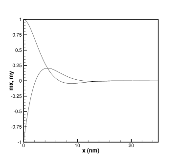
Figure 1: ZLF solution for a half-plane geometry. The x and y components are normalized to one.

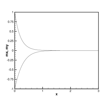
Figure 2: Our solution for a half-plane geometry for the same parameters as in Fig.1 (see text). The x and y components are normalized to one. Note the difference in scale along the x-axis (nm) with respect to fig.1.

References

- (1) L. Berger, Phys. Rev.B, 54, 9353 (1996); L. Berger, J. Apl.Phys., 89, 5521 (2001).
- (2) J. C. Slonczewski, J. Magn. Magn. Mater. 159, L1 (1996); J. C. Slonczewski, J. Magn. Magn. Mater. 247, 324 (2002).
- (3) J. A. Katine, F. J. Albert, R. A. Buhrman, E. B. Myers, and D. C. Ralph, Phys. Rev. Lett. 84, 3149 (2000).
- (4) W. Weber, S. Rieseen, and H. C. Siegmann, Science 291, 1015 (2001).
- (5) C. Heide, P. E. Zilberman and R. J. Elliott, Phys. Rev. B 63, 64424 (2001); C. Heide, Phys. Rev. Lett. 87, 197201 (2001).
- (6) Ya. B. Bazaliy, B. A. Jones, and S.-C. Zhang, Phys. Rev.B 57, R3213 (1998).
- (7) X. Waintal, E. B. Myers, P. W. Brouwer, and D. C. Ralph, Phys. Rev. B 62, 12317 (2000).
- (8) A. Brataas, Y. V. Nazarov and G. E. Bauer, Eur. Phys. J.B 22, 99 (2001); A. A. Kovalev, A. Brataas and G. E. W. Bauer, Phys. Rev. B 66 224424 (2002).
- (9) S. Zhang, P. M. Levy, A. Fert, Phys. Rev. Lett. 88, 236601 (2002); A. Shpiro, P. M. Levy and S. Zhang, Phys. Rev. B 67, 104430 (2003).
- (10) M. D. Stiles, A. Zangwill, Phys. Rev. B 66, 014407, (2002).
- (11) E. Simanek and B. Heinrich, Phys. Rev. B 67, 144418 (2003).
- (12) D. L. Mills, Phys. Rev. B 68, 014419 (2003).
- (13) J. Ho, F.C. Khanna and B. C. Choi, Phys. Rev. Lett. 92, 097601 (2004).
- (14) R. Chantrell and A. Rebei, unpublished.
- (15) T. Valet and A. Fert, Phys. Rev. B 48, 7099 (1993).
- (16) W.N.G. Hitchon, G. J. Parker and A. Rebei, (to be published).
- (17) J. Schwinger, J. Math. Phys. 2, 407 (1961).
- (18) H. Haug and A.-P. Jauho, Quantum Kinetics in Transport and Optics of Semiconductors, Springer, Berlin, 1996.
- (19) I. I. Hirst, Phys. Rev. 141, 503 (1966).
- (20) J. I. Kaplan, Phys. Rev. 143, 351 (1966).
- (21) A. Rebei and M. Simionato, unpublished.
- (22) M. Zwierzycki, Y. Tserkovnyak, P. J. Kelly, A. Brataas and G. E. Bauer, cond-mat/0402088