Dielectric anomaly in coupled rotor systems

Abstract

The correlated dynamics of coupled quantum rotors carrying electric dipole moment is theoretically investigated. The energy spectra of coupled rotors as a function of dipolar interaction energy is analytically solved. The calculated dielectric susceptibilities of the system show the peculiar temperature dependence different from that of isolated rotors.

I Introduction

With the advent of nanotechnologies, quantum rotors have attracted much attention in relevance to a fundamental element of molecular scale machinery Gimzewski ; Koumura ; Bermudez . Arrays of surface mounted quantum rotors with electric dipole moments are of particular interest because dipole-dipole interactions can be controlled and even designed to yield specific behavior, such as ferroelectricity. Ordered two-dimensional arrays of dipole rotors yield either ferroelectric or antiferroelectric ground states, depending on the lattice type, while disordered arrays are predicted to form a glass phase Rozen1988 ; Rozen1991 .

Besides technological problems, the microscopic dynamics of quantum rotors have extensively studied from physical and chemical interest. The idea of quantum rotors is applicable to interstitial oxygen impurities in crystalline germanium, where oxygen atoms are quantum-mechanically delocalized around the bond center position Artacho97 . The rotational of oxygen impurities around the Ge-Ge axis has been experimentally observed by phonon spectroscopy Gienger . While the rotation of oxygen impurities in Ge is weakly hindered by an azimuthal potential caused by the host lattice, several materials are known to show a free rotation of molecules. An example is ammonia groups in certain Hofmann clathrates M(NH₃)₂M’(CN)₄-G Wegener ; Kearley ; Vorderwisch , usually abbreviated as M-M’-G, where M and M’ are divalent metal ions and G is a guest molecule. Nearly free uniaxial quantum rotation of NH₃ has been observed for the first time in Ni-Ni-(C₆D₆)₂ by inelastic neutron scattering Wegener . Recently, a surprising variation of the linewidth has been observed for Ni-Ni-(C₁₂H₁₀)₂ Rogalsky , which has been interpreted by a novel line broadening mechanism based on rotor-rotor coupling Wurger . It is also known that the $\beta$ phase of solid methane Press as well as methane hydrate Gutt show almost free rotation of CH₄ molecule. The linewidths of methane in clathrates show inhomogeneous broadening owing to the dipolar coupling with water molecules Gutt2 . It is therefore expected that new interesting phenomena will be found by investigating the influence of dipolar interaction between quantum rotors.

In the present paper, we study the correlated dynamics of coupled quantum rotors carrying electric dipole moments. We give the exact solution of eigenvalue problem of interacting rotors with arbitrary configurations. It is revealed that coupled rotors show a peculiar dielectric response at low temperatures, which can be interpreted by taking account of the selection rule of dipolar transition for coupled rotors.

II The Hamiltonian

Figure 1: Schematic configuration of coupled rotors. Each rotors represented by $\bm{r}_{1}$ and $\bm{r}_{2}$ rotates along a ring of a radius $r$, and carry dipole moment $q\bm{r}_{1\,(2)}$.

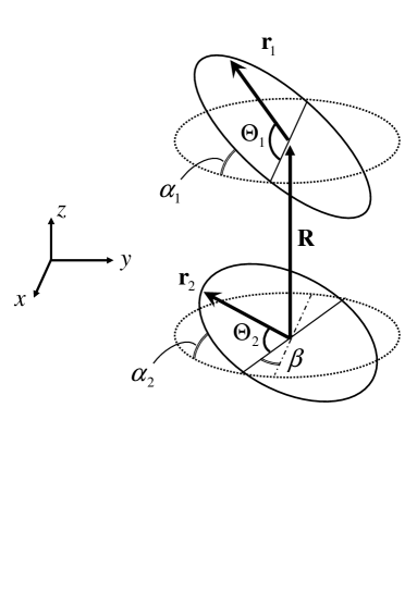
Suppose two dipole rotors $q\bm{r}_{1}$ and $q\bm{r}_{2}$ separated by the vector $\bm{R}$. The Hamiltonian for the system is given by $H=H_{K}+W_{D}$, where the kinetic term is

$$H_{K}=-\frac{\hbar^{2}}{2I}\left(\frac{\partial^{2}}{\partial\Theta_{1}^{2}}+\frac{\partial^{2}}{\partial\Theta_{2}^{2}}\right),$$ (1)

and the interaction term becomes

$$W_{D}=\frac{q^{2}}{4\pi\varepsilon}\left(\frac{1}{|\bm{R}|}+\frac{1}{|\bm{R}+\bm{r}_{1}-\bm{r}_{2}|}-\frac{1}{|\bm{R}+\bm{r}_{1}|}-\frac{1}{|\bm{R}-\bm{r}_{2}|}\right).$$ (2)

Here $I$ is the moment of inertia for dipole rotors and $\varepsilon$ the dielectric constant, respectively. Figure 1 shows a configuration of two dipoles rotors under consideration. We assume that rotors do not feel any potential variation along a ring of radius $r$. In the Jacobi coordinate, the vectors $\bm{r}_{1},\bm{r}_{2}$ and $\bm{R}$ are given by

$$\bm{r}_{1} = r(\cos\Theta_{1},\;\sin\Theta_{1}\cos\alpha_{1},\;\sin\Theta_{1}\sin\alpha_{1}),$$

$$\bm{r}_{2} = r(\cos\Theta_{2}\cos\beta-\sin\Theta_{2}\cos\alpha_{2}\sin\beta,\;$$

$$\quad\cos\Theta_{2}\sin\beta+\sin\Theta_{2}\cos\alpha_{2}\cos\beta,\;\sin\Theta_{2}\sin\alpha_{2}),$$

$$\bm{R} = R(0,\;0,\;1).$$ (3)

A spatial profile of $W_{D}$ as a function of $(\Theta_{1},\Theta_{2})$ is displayed in Fig. 2 by a contour plot, in which the angles $(\alpha_{1},\alpha_{2},\beta)$ are set as $(\pi/4,-\pi/6,\pi/3)$. We should remark that two minima (dark regions) and two maxima (white ones) are located at the anti-parallel or parallel dipolar configuration, indicating that the dipoles prefer an anti-parallel configuration. The two minima of $W_{D}(\Theta_{1},\Theta_{2})$ arise from the dipole interaction between two rotors, i.e., the dipole interaction plays a key role for creating barriers and two potential minima, which strongly affect the energy spectra and the dielectric response of the system.

Figure 2: Contour plot of the interaction term $W_{D}$ in $(\Theta_{1},\Theta_{2})$ plane. Two maxima (white regions) and two minima (dark regions) are realized at positions with differences $\Delta\Theta_{1}\approx\pi$ and $\Delta\Theta_{2}\approx\pi$. Parameter values are given in the text.

Provided that the spacing $R$ is large enough compared with the radius $r$, the interaction term $W_{D}$ can be expanded in terms of $1/R$. The lowest-order term has the form of a dipolar interaction given by

$$W_{D}^{(3)}=\frac{q^{2}}{4\pi\varepsilon R^{3}}\left\{\bm{r}_{1}\cdot\bm{r}_{2}-\frac{3(\bm{r}_{1}\cdot\bm{R})(\bm{r}_{2}\cdot\bm{R})}{R^{2}}\right\}.$$ (4)

The higher-order term $W_{D}^{(4)}\equiv W_{D}-W_{D}^{(3)}$ is of the order of $O(r^{3}/R^{4})$, which can be negligible for the case $R\gg r$. Actually we have confirmed that the calculated results presented in this paper change very little by taking into account the term $W_{D}^{(4)}$.

III Eigenvalues and eigenfunctions

The Schrödinger equation for the Hamiltonian $H_{0}=H_{K}+W_{D}^{(3)}$ has analytic solutions as shown below. Transforming variables to $\theta_{1}=(\Theta_{1}+\Theta_{2})/2$ and $\theta_{2}=(\Theta_{1}-\Theta_{2})/2$, Eqs. (1) and (4) yields

$$H_{K} = -\frac{\hbar^{2}}{4I}\left(\frac{\partial^{2}}{\partial\theta_{1}^{2}}+\frac{\partial^{2}}{\partial\theta_{2}^{2}}\right),$$ (5)

$$W_{D}^{(3)} = \frac{q^{2}r^{2}}{4\pi\varepsilon R^{3}}\sum_{i=1}^{2}c_{i}\cos 2(\theta_{i}+\gamma_{i}).$$ (6)

The parameters $c_{i}$ and $\gamma_{i}$ $(i=1,2)$ are functions of angles $\alpha_{1},\alpha_{2}$ and $\beta$ defined in Fig. 1, whose explicit forms are given by

$$c_{i}=\frac{1}{2}\sqrt{x_{i}^{2}+y_{i}^{2}},\quad\gamma_{i}=\frac{1}{2}\tan^{-1}\left(\frac{-x_{i}}{y_{i}}\right),$$ (7)

with the definitions

$$x_{1} = \sin\beta(\cos\alpha_{1}-\cos\alpha_{2}),$$

$$x_{2} = \sin\beta(\cos\alpha_{1}+\cos\alpha_{2}),$$

$$y_{1} = \cos\beta(1-\cos\alpha_{1}\cos\alpha_{2})+2\sin\alpha_{1}\sin\alpha_{2},$$

$$y_{2} = \cos\beta(1+\cos\alpha_{1}\cos\alpha_{2})-2\sin\alpha_{1}\sin\alpha_{2}.$$ (8)

Consequently, we can decompose the Schrödinger equation $H_{0}\varPsi_{0}(\theta_{1},\theta_{2})=E_{0}\varPsi_{0}(\theta_{1},\theta_{2})$ into two independent Mathieu equations. Setting $\varPsi_{0}(\theta_{1},\theta_{2})=\varphi_{1}(\theta_{1})\varphi_{2}(\theta_{2})$, we obtain

$$-\frac{\partial^{2}\varphi_{i}}{\partial\theta_{i}^{2}}+\frac{2}{E_{K}}\left[c_{i}E_{D}\cos 2(\theta_{i}+\gamma_{i})-E_{i}\right]\varphi_{i}=0,\quad[i=1,2]$$ (9)

where the quantities $E_{K}=\hbar^{2}/(2I)$ and $E_{D}=q^{2}r^{2}/(4\pi\varepsilon R^{3})$ represent the kinetic and interaction energy, respectively. The eigenvalue $E$ of the initial Schrödinger equation is expressed as the sum of $E=E_{1}+E_{2}$. Note that the periodic terms $\propto\cos 2(\theta_{i}+\gamma_{i})$ originate from two minima (or maxima) of the interaction term $W_{D}(\Theta_{1},\Theta_{2})$ shown in Fig. 2 foot1 .

Eigenfunctions of Eq.(9) are described by four types of the Mathieu functions, given by ce${}_{2n}(v_{i},\theta_{i})$, se${}_{2n+1}(v_{i},\theta_{i})$, ce${}_{2n+1}(v_{i},\theta_{i})$ and se${}_{2n+2}(v_{i},\theta_{i})$ with the definitions $v_{i}\equiv c_{i}E_{D}/E_{K}$ and $n=0,1,2\cdots$. Each of them belongs to a different eigenvalue and can be expressed in terms of the Fourier-cosine expansion; for instance,

$${\rm ce}_{2n}(v_{i},\theta_{i})=\sum_{m=0}^{\infty}A_{2m}^{(2n)}(v_{i})\cos 2m(\theta_{i}+\gamma_{i}).$$ (10)

The coefficients $\{A_{2m}^{(2n)}\}$ are determined by a successive relation obtained by substituting Eq.(10) into Eq.(9). The amplitudes of $\{A_{2m}^{(2n)}\}$ rapidly decrease with increasing $m$, so that we can truncate the summation in Eq. (10) at $m=20$ in actual calculations.

Figure 3: The energy spectra of the paired-rotor as a function of $E_{D}$. Solid arrows indicate a part of allowed dipole transitions for the component $p_{x}$ in the case of $(\alpha_{1},\alpha_{2},\beta)=(\pi/4,0,0)$. The explanation on three labels (a)-(c) is given in text.

Figure 3 plots the calculated spectra of eigenenergies $E=E_{1}+E_{2}$ as a function of $E_{D}$, where $E_{K}$ is taken as an energy unit. The angles $(\alpha_{1},\alpha_{2},\beta)$ are set to be $(\pi/4,0,0)$ as an example. We find, though some levels are degenerate when $E_{D}=0$, they split off for finite $E_{D}$ with a monotonous variation with increasing $E_{D}$. For high-$E_{D}$ limit, some levels become degenerate again. It indicates that the relative motion of paired-rotors is frozen out for $E_{D}\gg E_{K}$ due to the strong Coulomb interaction. This behavior can be understood from the spatial profile of the interaction term $W_{D}(\Theta_{1},\Theta_{2})$ shown in Fig. 2. With increasing $E_{D}$, the depths of two minima of $W_{D}(\Theta_{1},\Theta_{2})$ grow, and larger barrier-heights hinder the quantum transition of a particle through the barrier. This gives rise to localized wavefunctions around these minima. Consequently, in the limit of $E_{D}\gg E_{K}$, the amplitude of the eigenfunctions are strongly localized around two minima, and these two localized eigenstates are nearly degenerate. Even if the higher-order term $W_{D}^{(4)}$ is taken into account, the energy spectra does not change much, since it only slightly disturbs the symmetry of the depths of two minima shown in Fig. 2. When varying the angles $(\alpha_{1},\alpha_{2},\beta)$, the curves in Fig. 3 slightly shift to upwards and/or downwards except for the unchanged values of $E$ at $E_{D}=0$.

IV Dielectric susceptibilities

Let us consider the dielectric response of dipole rotors coupled via dipolar interaction. The real part of the frequency-dependent dielectric susceptibility is expressed as

$$\chi_{\mu\mu}(\omega,T) = -\frac{2}{\varepsilon Z}\sum_{j,l\neq j}\left|\langle E_{j}|p_{\mu}|E_{l}\rangle\right|^{2}$$ (11)

$$\times \frac{E_{j}-E_{l}}{(E_{j}-E_{l})^{2}-(\hbar\omega)^{2}}\exp\left(-\frac{E_{j}}{k_{B}T}\right),$$

where $Z=\sum_{j}\exp(-E_{j}/k_{B}T)$ is the partition function, and $|E_{j}\rangle$ is the eigenvector belonging to the eigenvalue $E_{j}$. The quantity $p_{\mu}$ is the $\mu$-component of the total dipole moment $\bm{p}=q(\bm{r}_{1}+\bm{r}_{2})$, which depend on the relative orientation with respect to the external field. We should note that the susceptibility depends on the selection rules for dipole transitions between different eigenstates. In Fig. 3, allowed dipole transitions for $p_{x}$ are indicated in part by solid arrows. Note that only a part of allowed transitions are shown in the figure, which are dominant for the dielectric susceptibility $\chi(\omega,\,T)$ at temperatures $T\approx E_{K}/k_{B}$. The rest of allowed dipolar transitions do not contribute to the susceptibility given by Eq.(11), because the energy difference $|E_{j}-E_{l}|$ is so large and/or the Boltzmann factor $\exp(-E_{j}/k_{B}T)$ become much smaller than unity. The interpretation on three labels (a)-(c) shown in Fig. 3 will be given later.

Figure 4: The dielectric susceptibility $\chi_{xx}(T)$ for the zero-frequency limit $\omega\to 0$ as a function of the inverse temperature $1/T$. The strength of dipolar interaction is increased from top to bottom; i) $E_{D}=0$ (solid), ii) $E_{D}=0.01$ (dashed), iii) $E_{D}=0.1$ (dash-dotted), and iv) $E_{D}=1.0$ (dotted) in units of $E_{K}$. Bumps at around $E_{K}/(k_{B}T)\approx 5.0$ appear in the cases of ii) and iii). Inset shows three components of $\eta_{j,l}(T)$ for the case of iii), whose definitions are given in text.

We have calculated the temperature dependence of the dielectric susceptibility $\chi_{\mu\mu}(\omega,T)$ for various $E_{D}$. Figure 4 shows the calculated results of dc susceptibility $\chi_{xx}(T)$ normalized by a factor $q^{2}r^{2}/(\varepsilon E_{K})$. We have taken four values of $E_{D}/E_{K}$; the solid line ($E_{D}=0$), the dashed one ($E_{D}/E_{K}=0.01$), the dash-dotted one ($E_{D}/E_{K}=0.1$), and the dotted one ($E_{D}/E_{K}=1.0$). The angles are set to be $(\alpha_{1},\alpha_{2},\beta)=(\pi/4,0,0)$ for all $E_{D}$. For the case of $E_{D}=0$, the susceptibility monotonically increases with decreasing temperature, and becomes constant at lower temperatures. The crossover temperature between the steady increase and the almost constant value in Fig. 4 is determined by the minimum-energy difference of eigenstates at $E_{D}=0$ that are allowed for dipole transition, namely, indicated as (a) in Fig. 3. For the case of $E_{D}/E_{K}>1$, the strong Coulomb interaction prevents from the relative motion of rotors so that the magnitude of the susceptibility $\chi(T)$ decreases with increasing $E_{D}$.

It is noteworthy that, for relatively weak interaction $E_{D}/E_{K}<0.1$, a bump is appeared in the susceptibility at about $E_{K}/(k_{B}T)\approx 5.0$. The kinetic energy $E_{K}=\hbar^{2}/(2I)$ for actual rotating molecules is the order of 1 meV Gutt , indicating that the characteristic temperature $T^{*}=E_{K}/k_{B}\times 0.2$ corresponding to the bump is estimated as about 1 K. We made sure that the bump can be observed for any angles $(\alpha_{1},\;\alpha_{2},\;\beta)$ when $E_{D}/E_{K}$ is less than $0.1$. This anomaly stems from the correlated rotation of paired-rotors via the dipolar interaction, and can be interpreted by the argument on the selection rule for dipolar transition.

To understand the origin of the bump, we decompose the total susceptibility $\chi_{xx}(T)$ give in Eq.(11) as

$$\chi_{xx}(T) = \sum_{(j,l\neq j)}\eta_{j,l}(T),$$ (12)

$$\eta_{j,l}(T) = -\frac{2}{\varepsilon Z}\frac{\left|\langle E_{j}|p_{x}|E_{l}\rangle\right|^{2}}{E_{j}-E_{l}}$$ (13)

$$\times \left[\exp\left(-\frac{E_{j}}{k_{B}T}\right)-\exp\left(-\frac{E_{l}}{k_{B}T}\right)\right],$$

where $\sum_{(j,l\neq j)}$ is the summation over all possible combinations of $(j,l)$ under the condition $l\neq j$. Note the fact that only three components of $\eta_{j,l}(T)$ are responsible for the total susceptibility (12) around the characteristic temperature $T^{*}$. We denote those components by $\eta^{a}$, $\eta^{b}$, and $\eta^{c}$, which are characterized by the eigenfunction $\varPsi_{j}=\langle\theta_{1},\theta_{2}|E_{j}\rangle$ and $\varPsi_{l}=\langle\theta_{1},\theta_{2}|E_{l}\rangle$ as follows;

$$\eta^{a}; \varPsi_{j}={\rm ce}_{0}(\theta_{1}){\rm ce}_{0}(\theta_{2}),\;\;\varPsi_{l}={\rm ce}_{1}(\theta_{1}){\rm ce}_{1}(\theta_{2}),$$ (14)

$$\eta^{b}; \varPsi_{j}={\rm ce}_{0}(\theta_{1}){\rm ce}_{1}(\theta_{2}),\;\;\varPsi_{l}={\rm ce}_{1}(\theta_{1}){\rm ce}_{0}(\theta_{2}),$$ (15)

$$\eta^{c}; \varPsi_{j}={\rm se}_{1}(\theta_{1}){\rm se}_{2}(\theta_{2}),\;\;\varPsi_{l}={\rm se}_{2}(\theta_{1}){\rm se}_{1}(\theta_{2}).$$ (16)

The alphabets subscribed on $\eta$ correspond to three dipolar transitions labeled by (a)-(c) shown in Fig. 3. For example, the solid arrow of (a) in Fig. 3 connects the eigenstates $\varPsi_{j}$ and $\varPsi_{l}$ defined in Eq.(14).

For weak coupling $E_{D}\ll E_{K}$, the solution of the Mathieu equation (9) is easily solved. In the lowest order of the perturbation theory, the eigenvalues $E_{i}(i=1,2)$ read in

$$E_{i}=\frac{E_{K}}{2}n^{2}+aE_{D}\quad(n=0,\pm 1,\pm 2,\cdots)$$ (17)

with a constant $a$. The solution (17) gives the eigenenergies of the states $|E_{j}\rangle$ and $|E_{l}\rangle$ relevant to the three components as follows;

$$\eta^{a};\;\quad(E_{j},E_{l}) = (0,E_{K}+\delta E_{a}),$$ (18)

$$\eta^{b};\;\quad(E_{j},E_{l}) = (\frac{E_{K}}{2}\pm\delta E_{b},\frac{E_{K}}{2}\mp\delta E_{b}),$$ (19)

$$\eta^{c};\;\quad(E_{j},E_{l}) = (\frac{5E_{K}}{2}\pm\delta E_{c},\frac{5E_{K}}{2}\mp\delta E_{c}).$$ (20)

The small corrections $\delta E$ stem from the small interaction energy $E_{D}\ll E_{K}$. Substituting these eigenenergies into Eq. (13), we find that the three components are approximated by

$$\eta^{a}(u) = \frac{2p_{a}^{2}}{\varepsilon E_{K}}\cdot\frac{1-e^{-u}}{Z(u)},$$ (21)

$$\eta^{b}(u) = \frac{2p_{b}^{2}}{\varepsilon E_{K}}\cdot\frac{ue^{-u/2}}{Z(u)},$$ (22)

$$\eta^{c}(u) = \frac{2p_{c}^{2}}{\varepsilon E_{K}}\cdot\frac{ue^{-5u/2}}{Z(u)},$$ (23)

where we defined $u=E_{K}/(k_{B}T)$. The quantities $p_{a}$, $p_{b}$ and $p_{c}$ equal to the value of $\left|\langle E_{j}|p_{x}|E_{l}\rangle\right|$ for the case of $\eta^{a}$, $\eta^{b}$ and $\eta^{c}$, respectively. The explicit form of the partition function $Z(u)$ is

$$Z(u)=1 + 4e^{-u/2}+4e^{-u}+4e^{-2u}+8e^{-5u/2}$$ (24)

$$+ 4e^{-4u}+4e^{-9u/2}+8e^{-5u}+\cdots,$$

which monotonically decreases with rasing $u$ and reaches unit for the limit $u\to\infty$. This means that the component $\eta^{a}(u)$ is a monotonic increase function of $u$. On the other hand, the components $\eta^{b}(u)$ and $\eta^{c}(u)$ is convex functions giving a maximum at finite $u$. The conditions of $u$ for the maximum of $\eta^{b}$ and $\eta^{c}$ are expressed by

$$1-\frac{u}{2}-u\frac{Z^{\prime}(u)}{Z(u)} = 0,\quad\mbox{for }\eta^{b},$$ (25)

$$1-\frac{5}{2}u-u\frac{Z^{\prime}(u)}{Z(u)} = 0,\quad\mbox{for }\eta^{c}.$$ (26)

The solutions of the Eqs. (25-26) is estimated as $u\approx 4$ for $\eta^{b}$ and $u\approx 0.5$ for $\eta^{c}$. Since the total susceptibility $\chi(T)$ is given by the summation $\eta^{a}+\eta^{b}+\eta^{c}$, it is expected that the convex features of $\eta^{b}(u)$ and $\eta^{c}(u)$ cause in the bump of the total susceptibility at $u\approx 5$ shown in Fig. 4.

The argument is clarified by the numerical results shown in the inset of Fig. 4, where the $u$-dependence of the components for $E_{D}/E_{K}=0.1$ are displayed; $\eta^{a}$ (dashed-dotted), $\eta^{b}$ (dotted), $\eta^{c}$ (dashed-dotted-dotted), together with that of the total susceptibility $\chi=\eta^{a}+\eta^{b}+\eta^{c}$ (solid). The component $\eta^{b}$ clearly shows a maximum at $u\approx 4$, whereas the contribution of $\eta^{c}$ is negligible due to the factor $e^{-5u/2}$ in Eq. (23). As a result, the summation $\eta^{a}(u)+\eta^{b}(u)$ shows a bump at $u=5.0$, which is the origin of the anomalous bump of the total susceptibility $\chi(T)$ at the characteristic temperature $T^{*}=E_{K}/k_{B}\times 0.2$. We should note here that, if quantum rotors are not interacting at all, the component $\eta^{b}$ exactly vanished due to the degeneracy $E_{j}=E_{l}=E_{K}/2$ (See Eq. (19)) and only the component $\eta^{a}$ is dominant for the total susceptibility $\chi(T)$. This means that the total susceptibility is a monotonic function as the same as $\eta^{a}$ so that the bump does not emerge. The anomalous bump of the susceptibility, therefore, manifests the relevance of the dipolar interaction to the dielectric response of quantum rotors.

V Conclusions

It is important to recall experiments reported in Ref. Enss2 , for the dielectric susceptibility of KCl crystals with Li defects. It has been found that the susceptibility does not scale linearing with the Li concentration, and even becomes smaller with increasing the concentration ($\approx 1000$ ppm), where the interaction between defects becomes relevant. In addition, a bump of the susceptibility is observed at about 200 mK for concentrations of 200-1000 ppm. These temperature dependences of the susceptibility together with the bumps are recovered well by our results shown in Fig. 4. Noting that defects in both systems move along closed loops and correlated each other, it is natural to assume that the similar picture holds. For a quantitative discussion, of course, one should take into account the effect of potential variation hindering the free rotation of Li⁺, which is caused by the Coulomb interaction between a mobile Li⁺ ion and the host atoms K⁺ and Cl^-. The problem has been theoretically investigated in Ref. Wurger2 ; Wurger3 based on the two-level tunneling model.

In conclusion, we have investigated the quantum dynamics of two dipole rotors coupled via dipolar interaction. By solving analytically the eigenvalue problem of coupled rotors, we have demonstrated the energy spectra of coupled rotors as a function of dipolar interaction. The anomalous temperature dependence of dielectric susceptibility is also shown. Our model is so general that it should be applicable in a variety of physical context relevant to quantum rotors.