Bulk and Collective Properties of a Dilute Fermi Gas in the BCS-BEC Crossover

Abstract

We investigate the zero-temperature properties of a dilute two-component Fermi gas with attractive interspecies interaction in the BCS-BEC crossover. We build an efficient parametrization of the energy per particle based on Monte Carlo data and asymptotic behavior. This parametrization provides, in turn, analytical expressions for several bulk properties of the system such as the chemical potential, the pressure and the sound velocity. In addition, by using a time-dependent density functional approach, we determine the collective modes of the Fermi gas under harmonic confinement. The calculated collective frequencies are compared to experimental data on confined vapors of ⁶Li atoms and with other theoretical predictions.

I Introduction

A hot topic in nowadays’ many-body physics is the study of Fermi gases at ultra-low temperature. Indeed, current experiments with atomic vapors are able to operate in the regime of deep Fermi degeneracy p1 ; p2 . The two-component Fermi gases of these experiments are dilute because the effective range $R_{0}$ of the interaction is much smaller than the mean interparticle distance, i.e. $k_{F}R_{0}\ll 1$ where $k_{F}=(3\pi^{2}n)^{1/3}$ is the Fermi wave vector and $n$ is the gas number density. Even in this dilute regime the s-wave scattering length $a$ can be very large: the interaction parameter $k_{F}a$ can be varied over a very wide range using the Feshbach resonance technique, which permits to vary the magnitude and the sign of $a$. The available experimental data on ⁶Li atoms are concentrated across the resonance, where $a$ goes from large negative to large positive values p3 ; p4 and where a crossover from a Bardeen-Cooper-Schrieffer (BCS) superfluid to a Bose-Einstein condensate (BEC) of molecular pairs has been predicted p5 ; p6 ; p7 .

In this paper we propose a reliable analytical fitting formula for the energy per particle of a homogeneous two-component Fermi gas, by analyzing the fixed-node Monte Carlo data of Astrakharchik et al. p8 . From this analytical formula it is straightforward to calculate several bulk properties of the system by means of standard themodynamical relations. This fitting formula enables us to calculate also the collective modes of the Fermi gas under harmonic confinement by using the hydrodynamic theory in the local-density approximation (LDA), including also a quantum pressure term. We compare our results with other theoretical predictions p9 ; p10 ; p11 ; p12 ; p13 ; p14 and, in particular, with the experimental frequencies of the collective breathing modes p3 ; p4 .

II Bulk properties

At zero temperature, the bulk energy per particle $\cal E$ of a dilute Fermi gas can be written as

$${\cal E}={3\over 5}\epsilon_{F}\;\epsilon(x)\;,$$ (1)

where $\epsilon_{F}=\hbar^{2}k_{F}^{2}/(2m)$ is the Fermi energy and $\epsilon(x)$ is a yet unknown function of the interaction parameter $x=k_{F}a$. In the weakly attractive regime ($-1\ll x<0$) one expects a BCS Fermi gas of weakly bound Cooper pairs. As the superfluid gap correction is exponentially small, the function $\epsilon(x)$ should follow the Fermi-gas expansion p15

$$\epsilon(x)=1+{10\over 9\pi}x+{4(11-2\ln{(2)})\over 21\pi^{2}}x^{2}+...\;.$$ (2)

In the weak BEC regime ($0<x\ll 1$) one expects a weakly repulsive Bose gas of dimers. Such Bose-condensed molecules of mass $m_{M}=2m$ and density $n_{M}=n/2$ interact with a positive scattering length $a_{M}=0.6a$, as predicted by Petrov et al. p16 . In this regime, after subtraction of the molecular binding energy, the function $\epsilon(x)$ should follow the Bose-gas expansion p17

$$\epsilon(x)={5\over 18\pi}{a_{M}\over a}x\left[1+{128\over 15\sqrt{6\pi^{2}}}\left({a_{M}\over a}\right)^{3/2}x^{3/2}+...\right]\;.$$ (3)

In the so-called unitarity limit ($x=\pm\infty$) one expects that the energy per particle is proportional to that of a non-interacting Fermi gas p18 . The fixed-node diffusion Monte-Carlo calculation of Astrakharchik et al. p8 finds

$$\epsilon(x=\pm\infty)=0.42\pm 0.01\;,$$ (4)

while an analogous calculaton of Carlson et al. p19 gave $\epsilon(x=\pm\infty)=0.44\pm 0.01$. The calculation of Astrakharchik et al. p8 is quite complete and gives the behavior of the energy of system across the unitarity limit. It is a standard convention to use the inverse interaction parameter $y=1/x=1/(k_{F}a)$ as the independent variable. In Fig. 1 we plot the data of $\epsilon(y)$ reported by Astrakharchik et al. p8 ; p20 . On the basis of the data of Carlson et al. p19 , Bulgac and Bertsch p14 proposed the following behavior of $\epsilon(y)$ near $y=0$:

$$\epsilon(y)=\xi-\zeta\;y+...$$ (5)

with $\xi=0.44$ and $\zeta=1$ for both positive and negative $y$. The denser data of Ref. p8 suggest instead a continuous but not differentiable behavior of $\epsilon(y)$ near $y=0$, namely with $\xi=0.42$ and $\zeta=\zeta_{-}=1$ in the BCS region ($y<0$) but $\zeta=\zeta_{+}=1/3$ in the BEC region ($y>0$). As expected, for large $|y|$, the Monte-Carlo data shown in Fig. 1 follow the asymptotic trends of Eq. (1) and Eq. (2).

We propose here the following analytical fitting formula

$$\epsilon(y)=\alpha_{1}-\alpha_{2}\arctan{\left(\alpha_{3}\;y\;{\beta_{1}+|y|\over\beta_{2}+|y|}\right)}\;,$$ (6)

interpolating the Monte Carlo energy per particle and the limiting behaviors for large and small $|y|$. Here the parameter $\alpha_{1}$ is fixed by the value $\xi$ of $\epsilon(y)$ at $y=0$, the parameter $\alpha_{2}$ is fixed by the value of $\epsilon(y)$ at $y=\infty$, and $\alpha_{3}$ is fixed by the asymptotic $1/y$ coefficient of $\epsilon(y)$ at large $|y|$ (Eqs. (2) and (3)). The ratio $\beta_{1}/\beta_{2}$ is determined by the linear behavior $\zeta$ of $\epsilon(y)$ near $y=0$. The value of $\beta_{1}$ is then determined by minimizing the mean square deviation from the Monte-Carlo data p21 . Of course, we consider two different set of parameters: one set in the BCS region ($y<0$) and a separate set in the BEC region ($y>0$). Table 1 reports the values of these parameters.

	BCS ($y<0$)		BEC ($y>0$)
	expression	value	expression	value
$\alpha_{1}$	$\xi$	0.4200	$\xi$	0.4200
$\alpha_{2}$	$\frac{2}{\pi}(1-\alpha_{1})$	0.3692	$\frac{2}{\pi}\alpha_{1}$	0.2674
$\alpha_{3}$	$\frac{9\pi}{10}\alpha_{2}$	1.0440	$\frac{18\pi}{5}\alpha_{2}\frac{a_{M}}{a}$	5.0400
$\beta_{1}$	[fitted]	1.4328	[fitted]	0.1126
$\beta_{2}$	$\alpha_{2}\alpha_{3}\beta_{1}/\zeta_{-}$	0.5523	$\alpha_{2}\alpha_{3}\beta_{1}/\zeta_{+}$	0.4552

Table 1: Parameters of the fitting function (6).

Figure 1 compares this fitting function (solid curve) to the Monte Carlo data. For the sake of completeness, in Fig. 1 we also show the dotted curve obtained with the [2,2] Padé approximation of Kim and Zubarev p11 , based only on the asymptotes and the Monte-Carlo value p19 at $y=0$. Our parametric formula is more accurate, especially around $y=0$.

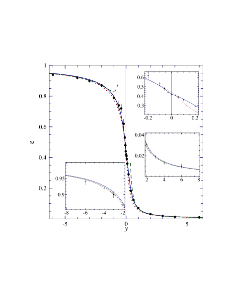
Figure 1: The energy per particle $\epsilon(y)$ as defined in Eq. (1), where $y=1/x=1/(k_{F}a)$. Solid circles represent the fixed-node Monte-Carlo data of Ref. p8 . Solid line is the parametric function (6) based on the values of Table 1. Dotted line is the Padé approximation of Ref. p11 . Dashed lines represent the asymptotic expressions Eq. (2) and Eq. (3).

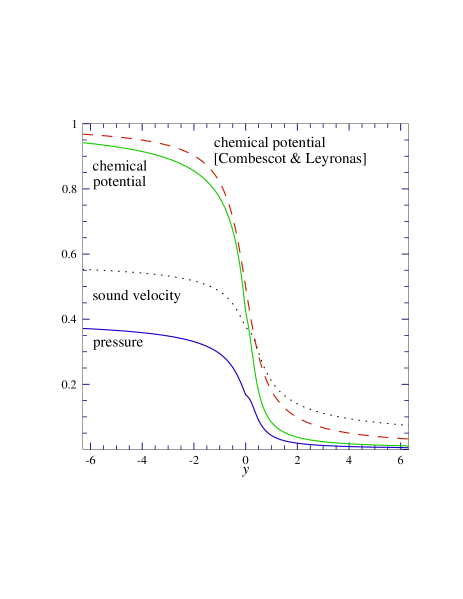
Figure 2: Chemical potential $\mu/\epsilon_{F}$, pressure $P/(n\epsilon_{F})$ and sound velocity $c_{s}/v_{F}$, obtained from the parametric function (6). Dashed line represents the simple model $\mu/\epsilon_{F}=\frac{1}{2}-\frac{1}{\pi}\arctan(\pi y/2)$ of Ref. p12 .

The advantage of a functional parametrization of $\epsilon(y)$ is that it allows straightforward analytical calculations of several ground-state physical properties of the bulk Fermi gas p22 . For example, the chemical potential $\mu$ is given by

$$\mu={\partial(n{\cal E})\over\partial n}=\epsilon_{F}\left(\epsilon(y)-{y\over 5}\epsilon^{\prime}(y)\right)\;,$$ (7)

as found by using Eq. (1) and taking into account that $\partial y/\partial n=-y/(3n)$, while the pressure $P$ reads

$$P=n^{2}{\partial{\cal E}\over\partial n}=n\;\epsilon_{F}\left({2\over 5}\epsilon(y)-{y\over 5}\epsilon^{\prime}(y)\right)\;.$$ (8)

The sound velocity $c_{s}$ is instead obtained as $c_{s}^{2}=(n/m)\partial\mu/\partial n$, from which we get

$$c_{s}=v_{F}\;\sqrt{{1\over 3}\epsilon(y)-{y\over 5}\epsilon^{\prime}(y)+{y^{2}\over 30}\epsilon^{\prime\prime}(y)}\;,$$ (9)

where $v_{F}=(2\epsilon_{F}/m)^{1/2}$ is the Fermi velocity. Figure 2 reports the chemical potential $\mu$, the pressure $P$ and the sound velocity $c_{s}$ as a function of $y$. Our theory predicts that all these macroscopic properties show a kink at the unitarity point, due to $\zeta_{-}\neq\zeta_{+}$. Figure 2 shows also the curve of the chemical potential obtained with the simple analytical model proposed by Combescot and Leyronas p12 . The sound velocity $c_{s}$ is accessible experimentally, and the dotted curve of Fig. 2 is our prediction of the way $c_{s}$ evolves from $v_{F}/\sqrt{3}$ to zero through the BCS-BEC crossover.

III Harmonically confined gas

We consider now the effect of confinement due to an external anisotropic harmonic potential

$$U({\bf r})={m\over 2}\left(\omega_{\rho}^{2}\rho^{2}+\omega_{z}^{2}z^{2}\right)\;,$$ (10)

where $\omega_{\rho}$ is the cylindric radial frequency and $\omega_{z}$ is the cylindric longitudinal frequency. Assuming that the density field $n({\bf r},t)$ varies sufficiently slowly (this assumption is at the basis of the LDA), at each point ${\bf r}$ the gas can be considered in local equilibrium, and the local chemical potential is $\mu[n({\bf r},t)]$. Within the LDA, the dynamics can be described by means of the hydrodynamic equations of superfluids

$${\partial n\over\partial t}+{\bf\nabla}\cdot(n{\bf v}) = 0\;,$$ (11)

$$m{\partial n\over\partial t}+\nabla\left(\mu[n({\bf r},t)]+U({\bf r})+{1\over 2}mv^{2}\right) = 0\;,$$ (12)

where ${\bf v}({\bf r},t)$ is the velocity field, and $\mu[n]$ is the chemical potential of Eq. (7). It has been shown by Cozzini and Stringari p23 that assuming a power-law dependence $\mu=\mu_{0}\;n^{\gamma}$ for the chemical potential (polytropic equation of state p12 ) from Eqs. (11-12) one finds analytic expressions for the collective frequencies. In particular, for the very elongated cigar-shaped traps used in recent experiments ($\omega_{r}/\omega_{z}>20$), the collective radial breathing mode frequency $\Omega_{\rho}$ is given by p23

$$\Omega_{\rho}=\sqrt{2(\gamma+1)}\;\omega_{\rho}\;,$$ (13)

while the collective longitudinal breathing mode $\Omega_{z}$ is

$$\Omega_{z}=\sqrt{3\gamma+2\over\gamma+1}\;\omega_{z}\;.$$ (14)

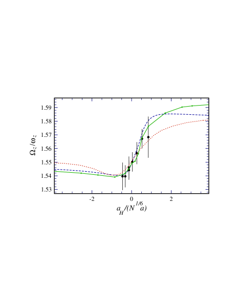
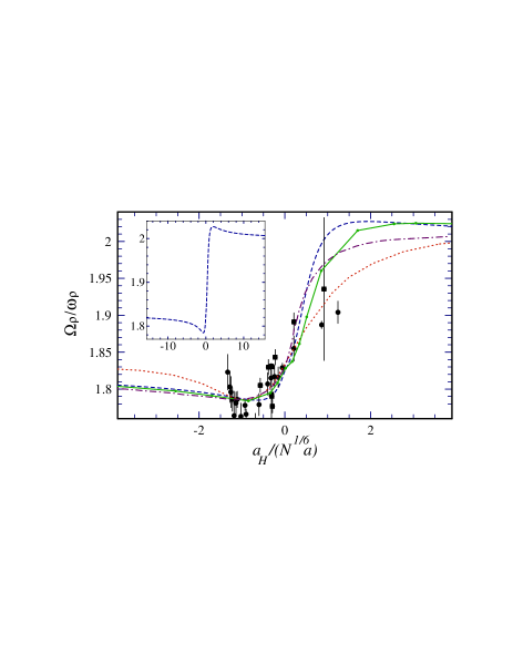
Figure 3: Frequencies of the longitudinal and radial collective breathing modes of the 2-component Fermi gas as a function of $a_{H}/(N^{1/6}a)=2^{1/2}3^{1/6}/(k_{F}a)=2^{1/2}3^{1/6}y$. $\Omega_{z}$ experimental data from Ref. p4 , and $\Omega_{\rho}$ experimental data from Ref. p3 a (squares) and Ref. p3 b (circles), both for ⁶Li. Joined dots with solid lines: TDDFT of Eq. (16), with $N=4\times 10^{5}$, $\omega_{\rho}/\omega_{z}=31.9$ for $\Omega_{z}$ and with $N=2\times 10^{5}$, $\omega_{\rho}/\omega_{z}=22.1$ for $\Omega_{\rho}$. Dot-dashed line: variational approximation to TDDFT, Ref. p11 . Dashed line: polytropic hydrodynamic approximation Eq. (13-14). Dotted line: the mean-field BCS of Ref. p10 .

In our problem we introduce an effective polytropic index $\gamma$ as the logarithmic derivative of the chemical potential $\mu$, that is

$$\gamma={n\over\mu}{\partial\mu\over\partial n}={{2\over 3}\epsilon(y)-{2y\over 5}\epsilon^{\prime}(y)+{y^{2}\over 15}\epsilon^{\prime\prime}(y)\over\epsilon(y)-{y\over 5}\epsilon^{\prime}(y)}\;.$$ (15)

We have verified that indeed $\gamma$ remains relatively close to unity for all $y$: the results of the local polytropic equation are thus useful to have a simple analytical prediction of the collective frequencies. Based on this polytropic hydrodynamic approximation (PHA), by using Eq. (6) we obtain the breathing-mode frequencies shown in Fig. 3 as dashed lines.

The analytical prediction of Eqs. (13-15) can be improved by releasing the polytropic approximation and explicitly integrating Eqs. (11-12). We have done such a calculation by including also a quantum pressure term $(-\hbar^{2}\nabla^{2}\sqrt{n})/(2m\sqrt{n})$ in Eq. (12). In practice, one must solve the following time-dependent nonlinear Schrödinger equation

$$i\hbar{\partial\over\partial t}\psi({\bf r},t)=\left[-{\hbar^{2}\over 2m}\nabla^{2}+U({\bf r})+\mu[n({\bf r},t)]\right]\psi({\bf r},t)\;,$$ (16)

where $\psi({\bf r},t)$ is the superfluid wave function such that $n({\bf r},t)=|\psi({\bf r},t)|^{2}$, ${\bf v}=\hbar\,\nabla\ln(\psi/n^{1/2})/(im)$, and $\mu[n]$ is the chemical potential of Eq. (7). Equation (16) can be interpreted as the Euler-Lagrange equation of a time-dependent density functional theory (TDDFT) p11 . In Ref. p11 , Eq. (16) is approached via a variational scheme. Here instead, Eq. (16) is solved numerically by using a finite-difference Crank-Nicolson predictor-corrector scheme p24 . First we obtain the ground state by integrating Eq. (16) in imaginary time. Then we let a slightly perturbed wave function evolve in real time for approximately one period of oscillation of the lowest (longitudinal) frequency $\Omega_{z}$. In the same time span, the density also undergoes several radial oscillations of frequency $\Omega_{\rho}$. We extract both frequencies by fitting the mean square widths of $n({\bf r},t)$ with the sum of two cosines. The breathing-mode frequencies obtained in this way are shown in Fig. 3 as dots joined by solid lines.

The quantum pressure term is important for small number of atoms, as it improves the determination of the density profile close to the surface of the vapor cloud p11 . For the number of particles of the experiments ($N\gtrsim 10^{5}$), the quantum pressure term is a relatively small correction, and according to our calculation it accounts for about $0.5\%$ of the total energy.

Figure 3 shows substantial accord between PHA and TDDFT. The main difference is the location of the predicted maximum in the bosonic region $y>0$. The differences are not only due to the approximations involved in the PHA, but also to numerical errors in TDDFT introduced by space and time discretization (estimated to less than 1%)p25 . We observe that, according to our predictions, the collective frequencies reach the asymptotic large-$|y|$ limits more slowly than the theory of Hu et al. p10 based on mean-field BCS Bogoliubov-de Gennes equations within LDA. In particular, in the BEC region, our numerical and analytical results (see the inset of Fig. 3) show that, contrary to the mean-field prediction, $\Omega_{\rho}$ approaches its asymptotic value $2\,\omega_{\rho}$ passing through a local maximum. $\Omega_{z}$ has the same nonmonotonic behavior while reaching $\sqrt{5/2}\,\omega_{z}$ for large $y$. This qualitative behavior was previoulsy suggested by Stringari p9 . The different asymptotic behavior of the BCS mean-field frequencies is due to the neglect of beyond mean-field corrections. Note also that further discrepancies on the BEC side are due to the mean-field relation $a_{m}=2a_{s}$ rather than $a_{m}=0.6a_{s}$ as provided by four-body scattering p16 and used in our calculation. The $\Omega_{\rho}$ curve computed in Ref. p11 (dot-dashed line in Fig. 3) agrees rather well with our calculation.

Different theories are compared to the experimental data by Kinast et al. p3 for the radial mode $\Omega_{\rho}$ and those by Bartenstein et al. p4 for the longitudinal mode $\Omega_{z}$. In Fig. 3, we use the standard variable $a_{H}/(N^{1/6}a)=2^{1/2}3^{1/6}y$ and follow Ref. p26 to determine the scattering length $a$ as a function of the magnetic field $B$ near the Feshbach resonance:

$$a=a_{b}\left[1+\alpha(B-B_{0})\right]\left[1+{\Delta\over B-B_{0}}\right]\;,$$ (17)

where $B_{0}=83.4149$ mT, $a_{b}=-1405\;a_{0}$, $\Delta=30.0$ mT, and $\alpha=0.0040$ (mT)^-1. For the longitudinal frequency $\Omega_{z}$, our results are in quantitative agreement with the experimental data, not unlike the mean-field prediction. The accord is less good for the radial mode. Experimental uncertainty of the position of the resonant field $B_{0}$ could partly account for these discrepancies. In particular the upward feature near $a_{H}/(N^{1/6}a)\simeq-1.5$ has been related p3 ; p12 to the breaking of the Cooper pairs (due to sizeable ratio between the collective energy $\hbar\Omega_{\rho}$ and the gap energy $\Delta$ p12 ), causing a failure of the hydrodynamical approximation. Finite-temperature and non-LDA effects not taken into account in the theories could be relevant. Note also that the experimental situation is not completely clear. The experimental measurement of $\Omega_{\rho}$ performed by Bartenstein et al. p4 (not shown in Fig. 3) disagree with the data of Kinast et al. p3 . In particular, Bartenstein et al. p4 find $\Omega_{\rho}/\omega_{\rho}\simeq 1.6$ at the unitarity limit $y=0$, instead of the expected value $\Omega_{\rho}/\omega_{\rho}=\sqrt{10/3}=1.82$ obtained from Eq. (13) for $\gamma=2$, characteristic of the (renormalized) free Fermi gas.

IV Discussion

We propose analytic expressions for the equations of state of a uniform dilute Fermi gas across the BCS-BEC transition. These expressions are based on recent Monte-Carlo data and well-established asymptotic expansions. By using a hydrodynamic local-density approximation we include the effect of harmonic confinement. We compare the predictions of this approach with experimental frequencies of confined ⁶Li vapors. Other predicted physical quantites can be accessed by future experiments. The hydrodynamic approach is improved, to address small number of atoms, by including a quantum-pressure term. Indeed, our parametric formula (6) provides an accurate expression for the $\mu$ term in Eq. (16) through Eq. (7), which gives a better determination of the density and of the collective frequencies. This generalized quantum hydrodynamic approach, which takes into account the beyond-mean-field corrections, provides a reliable tool to determine the density profile of the Fermionic cloud and to investigate its collective dynamical properties, including also mode coupling and anharmonic oscillations.

References

- (1) M. Greiner, C.A. Regal, and D.S. Jin, Nature 426, 537 (2003).
- (2) S. Jochim, M. Bartenstein, A. Altmeyer, G. Hendl, S. Riedl, C. Chin, J.H. Denschlag, and R. Grimm, Science 302, 2101 (2003).
- (3) (a) J. Kinast, S.L. Hemmer, M.E. Gehm, A. Turlapov, and J.E. Thomas, Phys. Rev. Lett. 92, 150402 (2004); (b) J. Kinast, A. Turlapov, and J.E. Thomas, cond-mat/0408634.
- (4) M. Bartenstein, A. Altmeyer, S. Riedl, S. Jochim, C. Chin, J. Hecker Denschlag, and R. Grimm, Phys. Rev. Lett. 92, 203201 (2004).
- (5) A.J. Leggett, in Modern Trends in the Theory of Condensed Matter, Ed. A. Pekalski and R. Przystawa (Springer, Berlin, 1980); P. Nozières and S. Schmitt-Rink, J. Low Temp. Phys. 59, 195 (1985); J.R. Engelbrecht, M. Randeria, and C.A.R. Sa de Melo, Phys. Rev. B 55, 15153 (1997).
- (6) M. Marini, F. Pistolesi, and G.C. Strinati, Eur. Phys. J. B 1, 151 (1998); P. Pieri and G.C. Strinati, Phys. Rev. B 61, 15370 (2000).
- (7) M. Holland, S.J.J.M.F. Kokkelmans, M.L. Chiofalo, and R. Walser, Phys. Rev. Lett. 87, 120406 (2001); Y. Ohashi and A. Griffin, Phys. Rev. A 67, 063612 (2003).
- (8) G.E. Astrakharchik, J. Boronat, J. Casulleras, and S. Giorgini, cond-mat/0406113.
- (9) S. Stringari, Europhys. Lett. 65, 749 (2004).
- (10) H. Hu, X.-J. Liu, A. Minguzzi, and M.P. Tosi, cond-mat/0404012.
- (11) Y.E. Kim and A.L. Zubarev Phys. Rev. A 70, 033612 (2004).
- (12) R. Combescot and X. Leyronas, Phys. Rev. Lett. 93, 138901 (2004).
- (13) H. Heiselberg, Phys. Rev. Lett. 93, 040402 (2004).
- (14) A. Bulgac and G.F. Bertsch, cond-mat/0404687.
- (15) K. Huang and C.N. Yang, Phys. Rev. 105 767 (1957); T.D. Lee and C.N. Yang, Phys. Rev. 105 1119 (1957).
- (16) D.S. Petrov, C. Salomon, and G.V. Shlyapnikov, cond-mat/0309010.
- (17) T.D. Lee, K. Huang, and C.N. Yang, Phys. Rev. 106 1135 (1957).
- (18) G.A. Baker, Jr., Phys. Rev. C 60 054311 (1999). G.A. Baker, Jr., Int. J. Mod. Phys. B 15, 1314 (2001); H. Heiselberg, Phys. Rev. A 63, 043606 (2001).
- (19) J. Carlson, S.-Y. Chang, V.R. Pandharipande, and K.E. Schmidt, Phys. Rev. Lett. 91 050401 (2003); S.-Y. Chang, V.R. Pandharipande, J. Carlson, and K.E. Schmidt, Phys. Rev. A 70, 043602 (2004).
- (20) We thank S. Giorgini for making available to us the Monte-Carlo numerical data of .
- (21) Our parametric function has been inspired by the simpler, but much less accurate, model function proposed by Combescot and Leyronars p12 .
- (22) K. Huang, Statistical Mechanics (Wiley, New York, 1980).
- (23) M. Cozzini and S. Stringari, Phys. Rev. Lett. 91, 070401 (2003).
- (24) W.H. Press, S.A. Teukolsky, W.T. Vettering, and B.P. Flannery, Numerical Recipes in C++ (Cambridge Univ. Press, Cambridge 2002); E. Cerboneschi, R. Mannella, E. Arimondo, and L. Salasnich, Phys. Lett. A 249, 495 (1998); L. Salasnich, A. Parola and L. Reatto, Phys. Rev. A 64, 023601 (2001).
- (25) This accuracy is realized with a mesh of radiallongitudinal points, and a time step .
- (26) M. Bartenstein, A. Altmeyer, S. Riedl, R. Geursen, S. Jochim, C. Chin, J. Hecker Denschlag, R. Grimm, A. Simoni, E. Tiesinga, C.J. Williams, and P.S. Julienne, cond-mat/0408673.