Rashba spin splitting in quantum wires

Abstract

This article presents an overview of results pertaining to electronic structure, transport properties, and interaction effects in ballistic quantum wires with Rashba spin splitting. Limits of weak and strong spin–orbit coupling are distinguished, and spin properties of the electronic states elucidated. The case of strong Rashba spin splitting where the spin–precession length is comparable to the wire width turns out to be particularly interesting. Hybridization of spin–split quantum–wire subbands leads to an unusual spin structure where the direction of motion for electrons can fix their spin state. This peculiar property has important ramifications for linear transport in the quantum wire, giving rise to spin accumulation without magnetic fields or ferromagnetic contacts. A description for interacting Rashba–split quantum wires is developed, which is based on a generalization of the Tomonaga–Luttinger model.

1 Introduction

Spin–dependent transport in nanostructures has attracted a lot of interest [1, 2] recently. A familiar example are magnetoresistance effects in hybrid systems [3] consisting of magnetic and nonmagnetics parts, which have important applications [4] in present data–storage technology. In such magnetoelectronics devices, spin–dependent conductances arise due to the interplay between ferromagnetic exchange–field splitting and the Pauli principle. A finite spin polarization of electric current in the normal parts of a hybrid system is a prerequisite [5] for magnetoresistance to occur. Strong efforts are currently directed towards doing magnetoelectronics using the recently discovered diluted magnetic semiconductor materials [6].

Parallel to the pursuit of a semiconductor–magnetoelectronics paradigm, recent studies have focused on finding out how the quantum nature of spin can affect current flow, in particular, in nonmagnetic semiconductor nanostructures. The fundamentally relativistic coupling between charge carriers’ spin and orbital degrees of freedom turns out to give rise to a host of interesting, and sometimes counterintuitive, spin–dependent transport effects. Of special appeal is the Rashba spin splitting [7, 8] arising in semiconductor heterostructures due to structural inversion asymmetry [9, 10]. The possibility to tune its strength by external gate voltages was demonstrated experimentally [11, 12] and forms the basis for a spin–dependent field–effect–transistor (spinFET) design [13]. Early studies [14, 15] discussed magnetoelectric effects in two–dimensional electron systems with Rashba spin splitting. (See also recent related work [16, 17].) The possibility to induce spin accumulation, or a nonequilibrium magnetization, by applying an electric field only is very interesting from a basic–science point of view, and would certainly be of great importance for spintronics applications. In this review, we show how the interplay between quantum confinement and spin–orbit coupling in quasi–onedimensional (1D) systems leads to just such a situation [18].

We are focusing on the electronic structure, transport properties, and interaction effects in ballistic quantum wires with Rashba spin splitting present. In the following Section, we formally introduce the theoretical model under consideration. The limits of weak and strong spin–orbit coupling will be distinguished by comparison of the two fundamental length scales involved, namely the wire width $W$ and the Rashba spin–precession length $L_{\mathrm{so}}$. In Sec. 3, the spin properties of electronic states in quasi–1D subbands are revealed. Subband hybridization for the case of strong spin–orbit coupling turns out to result in an unusual spin structure where the direction of motion for electrons at the Fermi wave number basically fixes their spin state. This is in stark contrast to conventional wires where states for both spin species exist for either propagation direction. Quantum wires in the limit of strong spin–orbit coupling exhibit therefore particularly intriguing transport properties, discussed in detail in Sec. 4 based on the scattering–theory formalism of mesoscopic electron transport [19]. We find, e.g., that application of an external voltage can lead to a spin accumulation and concomitant spin–polarized current flow. Possibilities for experimental confirmation of our predictions will be elucidated. The quasi–1D subband structure obtained in Sec. 2 will form the basis for a description of interacting Rashba–split quantum wires in Sec. 5, based on generalizations of the Tomonaga–Luttinger model [20, 21]. Again, the interesting case is the one with strong spin–orbit coupling where the unusual spin properties of subband states result in peculiar properties of spin–sensitive correlation functions. We formulate our conclusions and give a brief outlook in the final Sec. 6.

2 Rashba spin splitting of quasi–1D subbands

The text–book example of a two–dimensional (2D) quantum well is now routinely realized by appropriate band–gap engineering in semiconductor heterostructures [22]. For low enough electron densities and temperatures, it is possible to describe the motion of electrons in the well using the Hamiltonian

$$H_{0}=\frac{1}{2m}\left(p_{x}^{2}+p_{y}^{2}\right)$$ (1)

of quasi–free particles in the lowest 2D subband. (We take the growth direction of the heterostructure to be the $z$ axis in our spatial coordinate system.) Corrections to this Hamiltonian which lead to a coupling of spin state and motion in real space arise, as in the three–dimensional bulk material, in the absence of inversion symmetry. In the quantum well, there exists an additional possibility for breaking inversion symmetry: creating an asymmetric band bending. For conduction–band states, the spin–orbit Hamiltonian resulting from this structural inversion asymmetry [23] has the form [7]

$$H_{\mathrm{so}}=\frac{\hbar k_{\mathrm{so}}}{m}\,\,\left(\vec{\sigma}\times\vec{p}\,\right)\cdot\hat{z}\quad.$$ (2)

Here $\vec{\sigma}$ denotes the vector of Pauli matrices, and the wave number $k_{\mathrm{so}}$ is a direct measure of the Rashba spin–orbit coupling strength. We use the latter as a phenomenological input parameter, which has to be determined experimentally [11, 12] or from spin–dependent electronic–structure calculations [24, 25, 26, 23]. The single–particle Schrödinger equation for the Hamiltonian $H_{\mathrm{2D}}=H_{0}+H_{\mathrm{so}}$ describing the 2D electronic motion can be solved straightforwardly [8]. Electronic eigenstates are labeled by a 2D wave vector $\vec{k}$ and the quantum number $\sigma=\pm 1$ of spin projection in the direction perpendicular to both $\vec{k}$ and the growth direction. The energy eigenvalues for states having the same $k=|\vec{k}|$ but opposite $\sigma$ turn out to differ by a zero–field spin splitting $\Delta E_{k}=\hbar^{2}k_{\mathrm{so}}k/m$. Unlike Zeeman splitting, to which it is often compared, Rashba spin splitting does not result in a finite global magnetization of the 2D electron system, as time–reversal symmetry is preserved by the Hamiltonian $H_{\mathrm{2D}}$. No common spin quantization axis can be found for its eigenstates. Furthermore, a cut through the energy dispersions reveals that spin bands are shifted not by a fixed energy, as is the case for Zeeman splitting, but rather in wave–vector direction. This is illustrated in Fig. 1.

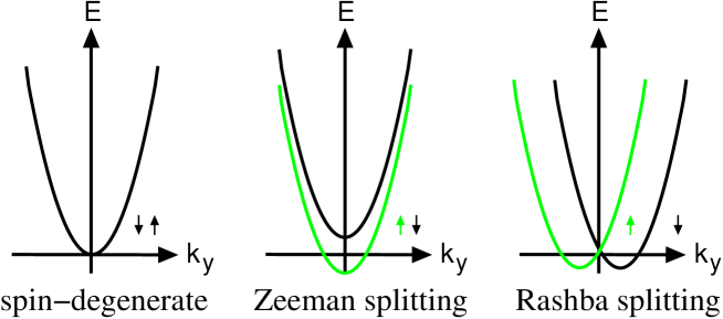
Figure 1: Comparison of Rashba and Zeeman spin splitting. Shown are energy dispersions for 2D single–electron eigenstates having a fixed $k_{x}=0$. Degenerate parabolic curves for both spin states get to be shifted in energy direction by an applied magnetic field. Quite differently, finite Rashba spin splitting results in wave–vector–shifted dispersion curves.

In the following, we are focusing exclusively on the situation where the motion of electrons is further confined to one spatial dimension by an external potential $V(x)$. To be specific, we assume a parabolic confinement

$$V(x)=\frac{m}{2}\,\,\omega^{2}\,x^{2}\quad,$$ (3)

as we can expect the qualitative features of spin splitting in quantum wires to be independent of the actual shape of the confining potential. In the absence of spin–orbit coupling, the single–electron spectrum is split into quasi–1D subbands having quadratic dispersion in the 1D wave vector $k_{y}$ that labels its eigenstates. The characteristic energy scale for subband bottoms is related to the width $W$ of the quantum wire. For finite $k_{\mathrm{so}}$, energy eigenstates are still plane waves in wire direction, but the linear dependence of $H_{\mathrm{so}}$ on the momentum $p_{x}$ in confinement direction introduces a coupling between the quasi–1D subbands. Using the 1D plane–wave representation, we can write the quantum–wire Hamiltonian in the form $H_{\mathrm{qw}}=H_{\mathrm{sb}}+H_{\mathrm{mix}}+H_{\mathrm{1D}}$, where

$$H_{\mathrm{sb}} = \frac{p_{x}^{2}}{2m}+V(x)\quad,$$ (4)

$$H_{\mathrm{mix}} = -\frac{\hbar k_{\mathrm{so}}}{m}\,\,\sigma_{y}\,p_{x}\quad,$$ (5)

$$H_{\mathrm{1D}} = \frac{\hbar^{2}}{2m}\left(k_{y}+k_{\mathrm{so}}\sigma_{x}\right)^{2}-\frac{\hbar^{2}k_{\mathrm{so}}^{2}}{2m}\quad.$$ (6)

The importance of quantum–wire subband coupling can be quantified by the ratio $s$ of the matrix elements of $H_{\mathrm{mix}}$ between eigenstates of $H_{\mathrm{sb}}+H_{\mathrm{1D}}$ (which describes a hypothetical quantum wire having only $p_{y}$–dependent spin splitting) and the difference of the corresponding eigen energies [27]. Estimating the parameter $s$ in terms of the wire width $W$, we find

$$s\approx\frac{\hbar k_{\mathrm{so}}}{m}\,\frac{\pi\hbar}{W}\left(\frac{\hbar^{2}\pi^{2}}{mW^{2}}\right)^{-1}=\frac{Wk_{\mathrm{so}}}{\pi}\equiv\frac{W}{L_{\mathrm{so}}}\quad,$$ (7)

where $L_{\mathrm{so}}$ is the spin precession length familiar from the proposed spinFET [13]. Hence two limits can be distinguished. (i) Quantum wire with weak Rashba spin splitting, realized for $W\ll L_{\mathrm{so}}$: Eigenstates are plane–wave spinors that are eigenstates of $\sigma_{x}$, i.e., have their spin polarized in the direction perpendicular to (and in the plane of) the wire. The energy dispersion is given by two parabolas, distinguished by the spin quantum number, that are shifted in wave–vector direction by an amount $2k_{\mathrm{so}}$. This is illustrated in Fig. 2a, which is essentially identical to the cut through a 2D Rashba–split dispersion shown in Fig. 1. (ii) Quantum wire with strong Rashba spin splitting, realized when $W\gtrsim L_{\mathrm{so}}$: Hybridization of quasi–1D subbands results in a nonparabolic energy dispersion [28, 27]. See Fig. 2b. In this case, no common spin quantum number can be assigned to states within a spin–split quantum–wire subband [18]. Their intriguing spin properties will be discussed in the following Section.

Figure 2: Quantum–wire subband dispersions in the limit of weak and strong Rashba spin splitting. (a) Parabolic dispersions shifted in wave–vector direction arise for weak spin splitting when the wire width is much smaller than the spin precession length. Each subband can be associated with a good quantum number of spin projection in the direction perpendicular to the wire. Data shown are for $\ell_{\omega}k_{\mathrm{so}}=0.1$. (b) In the opposite case of strong spin splitting, hybridization between adjacent subbands with opposite spin results in a nonparabolic dispersion. We show data for the case $\ell_{\omega}k_{\mathrm{so}}=0.9$.

A useful analytical result can be obtained for energy eigenvalues of states in a parabolic quantum wire having $k_{y}=0$. As $H_{\mathrm{1D}}$ vanishes in this case, these are eigenspinors of $\sigma_{y}$ whose components are eigenfunctions of harmonic oscillators with a spin–dependent boost. The energy eigenvalue is degenerate in the good quantum number of spin projection in the wire direction. With $l_{\omega}=\sqrt{\hbar/(m\omega)}$ denoting the oscillator length scale introduced by the parabolic wire confinement, it is explicitly given by

$$E_{n}(k_{y}=0)=\frac{\hbar\omega}{2}\left[2n+1-(\ell_{\omega}k_{\mathrm{so}})^{2}\right]\quad.$$ (8)

The spin–orbit correction to the energy of these states arises due to their finite quantized motion in the direction perpendicular to the wire. This exact result is an important benchmark to judge the accuracy of numerical methods that are necessary to obtain the full dispersion curves for all wave vectors [29].

3 Spin properties of quantum–wire eigenstates

While it is not possible to find a common spin quantization axis for eigenstates in a 2D system with Rashba spin splitting, restriction to one spatial propagation direction restores a global spin–projection axis for the case of weak spin–orbit coupling. In this limit, it is possible to neglect $H_{\mathrm{mix}}$, and the single–electron states in the wire are given, to a good approximation, by eigenstates of spin projection parallel to the wire confinement, i.e., the $x$ direction. At any given energy, there exist two such eigenstates with opposite spin, which have wave vectors differing by $2k_{\mathrm{so}}$. The effect of finite $H_{\mathrm{mix}}$ is to modify the local spin density of eigenstates across the wire, introducing a small zero–average tilt out of the wire plane [30]. This inhomogeneity of spin density as a function of the coordinate perpendicular to the wire becomes more important for strong spin–orbit coupling [18]. Still, direct experimental observation of this texture–like spin structure would be quite challenging.

The mixing term $H_{\mathrm{mix}}$ couples eigenstates obtained from diagonalizing $H_{\mathrm{sb}}+H_{\mathrm{1D}}$ which have opposite spin. In the special case of a parabolic confinement, its matrix elements turn out to be finite only between those opposite–spin states whose oscillator–band indices differ by one [31]. Hence, wherever the dispersion relations for such energetically adjacent subbands with opposite spin cross, $H_{\mathrm{mix}}$ cannot be neglected, as it will induce an anticrossing. Another way to define the limit of weak spin–orbit coupling is then to say that such anticrossings occur only at energies that are much higher than the typical quasi–1D subband splitting and, hence, can be neglected in the case when only a few wire subbands are occupied. As the parameter $s$ defined in Eq. (7) gets close to unity, anticrossings occur at energies comparable to those of low–lying wire subbands and affect its properties in an important way. Following the picture of anticrossings, it becomes immediately apparent that a peculiar spin structure emerges for states in hybridized subbands. In particular, their eigen–spin direction becomes a function of wave vector and is not uniform anymore within each band.

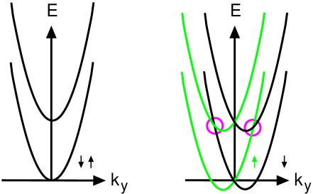
Figure 3: Effect of subband mixing in the limit of strong spin–orbit coupling. Shown in the left panel are two spin–degenerate subbands in the absence of Rashba spin splitting. Dispersions obtained from diagonalizing $H_{\mathrm{sb}}+H_{\mathrm{1D}}$ are parabolas shifted, due to Rashba spin splitting, in wave–vector direction, as shown in the right panel. Corresponding eigenstates have spin polarized in the direction perpendicular to the wire. The mixing Hamiltonian $H_{\mathrm{mix}}$ induces subband hybridization near crossing points, indicated on the right panel by circles. As a result, states in the lowest two spin–split subbands have approximately parallel spin at large wave vectors.

Consider the hybridization of the lowest two spin–split subbands, as illustrated in Fig. 3. The resulting nonparabolic dispersion for a particular parameter $l_{\omega}k_{\mathrm{so}}$ is given in Fig. 2b. Note that states in the lowest pair of subbands exist with wave vector larger than that for the crossing point but energies smaller than the bottoms of the next subband pair. These states originated from the first–excited spin–down subband but have become part of the lowest subband after hybridization. Their wave–vector distance to the crossing point is large enough such that the spin–up admixture in the eigenspinors is quite small. Hence we find a situation where right–moving states at still comfortably low energies in the lowest spin–split subbands have basically parallel spin! For the case depicted, there are basically only spin–down right–movers at large enough energies, and similarly only spin–up left–movers. This direct association of spin state with the direction of motion is peculiar to the strong–Rashba–split situation. In an ordinary quantum wire, even with Zeeman splitting or weak Rashba splitting present, there exist right–moving states for both spin–up and spin–down electrons at any energy. It can be envisioned that, for suitable parameter ranges, there exists a finite energy window for which even more than two sets of low–lying subbands have right–moving (and left–moving) states with almost parallel spin. This turns out to indeed be the case for $\ell_{\omega}k_{\mathrm{so}}=0.9$. In Fig. 4, we show the expectation value of the spin projection perpendicular to the wire for eigenstates in the lowest two pairs of spin–split quantum–wire subbands.

Figure 4: Spin projection of eigenstates in the lowest (a) and first excited (b) spin–split subbands for the situation when $\ell_{\omega}k_{\mathrm{so}}=0.9$. (See the corresponding dispersions in Fig. 2.) In both cases, states at large wave vector have approximately parallel spin.

In both sets of subbands, right–moving states at large wave vector exist only for spin–down electrons, and left–moving ones only for spin–up [32].

Exactly at the anticrossing, eigenstates of $H_{\mathrm{qw}}$ are the symmetric and antisymmetric superpositions of spin–up and spin–down states from the two intersecting quasi–1D subbands for $H_{\mathrm{sb}}+H_{\mathrm{1D}}$. Due to this peculiar mixing of spin and subband wave functions, expectation values of spin projected in any direction yields zero for quantum–wire eigenstates at the anticrossing. Their special spin properties turn out to give rise to an additional spin rotation of incoming electrons with energies within the anticrossing gap [38], which would enable enhanced performance of a suitably designed spinFET [39].

4 Spin–dependent transport from electric fields only

The key theoretical tool for studying linear transport in mesoscopic systems is the Landauer–Büttiker formalism [19], which is valid when electron–electron interaction is negligible. The central result of this approach is that the conductance of a mesoscopic sample can be related to the scattering matrix, $\mathcal{S}$, of the sample. In the spin–independent case, the scattering matrix is diagonal in spin space, and the problem can be mapped to scattering of spinless particles. Spin is then taken into account only as a factor $2$, and the linear conductance at zero temperature simply reads $G=\frac{2e^{2}}{h}\sum_{j\in 1,i\in 2}|\mathcal{S}_{i,j}|^{2}$, where $\mathcal{S}_{i,j}$ is the scattering amplitude (transmission coefficient) between the mode $j$ in terminal $1$ and the mode $i$ in terminal $2$. In this situation (spin–independent case), time–reversal symmetry implies $\mathcal{S}=\mathcal{S}^{\mathrm{T}}$, i.e., $\mathcal{S}_{i,j}=\mathcal{S}_{j,i}$, where, in the generic multi-terminal case, $i$ and $j$ are collective indices labeling both terminals and transverse modes. In the presence of spin–orbit coupling, there is no common spin quantization axis, and the full spin structure of $\mathcal{S}$ should be retained [40]. The total two-terminal conductance reads then $G=\frac{e^{2}}{h}\sum_{j\in 1,i\in 2,\sigma,\sigma^{\prime}}|\mathcal{S}_{i\sigma,j\sigma^{\prime}}|^{2}$, where $\sigma$ and $\sigma^{\prime}$ denote the spin projection along a common quantization axis. The spin–$\sigma$ current in the output contact $2$ is given by $I_{\sigma}=G_{\sigma}V$, where

$$G_{\sigma}=\frac{e^{2}}{h}\sum_{j\in 1,i\in 2,\sigma^{\prime}}|\mathcal{S}_{i\sigma,j\sigma^{\prime}}|^{2}\quad.$$ (9)

In Eq. (9) the sum over the transmission probabilities for different incoming spin projections $\sigma^{\prime}$ describes the fact that the injecting reservoir $1$ is not spin–polarized. In this case of a nondiagonal scattering matrix in spin space, the condition satisfied by the scattering matrix due to time–reversal symmetry reads

$$\mathcal{S}_{i\sigma,j\sigma^{\prime}}=(\sigma\sigma^{\prime})\mathcal{S}_{j-\sigma^{\prime},i-\sigma},$$ (10)

where $\sigma$ and $\sigma^{\prime}$ denote the spin projection along a common quantization axis and can take the values $\pm 1$. The condition Eq. (10) does not forbid the creation of spin-polarized currents in linear transport.

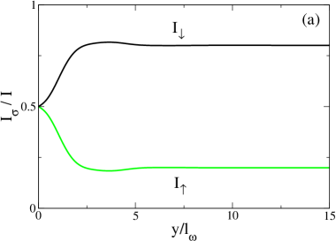
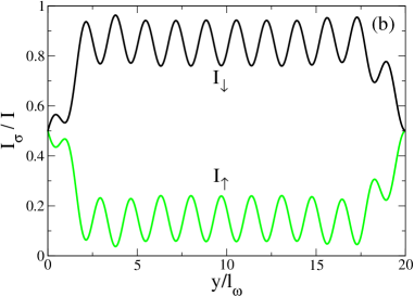
Figure 5: Transport in the hybrid wire/leads system computed by means of Landauer–Büttiker formalism. The total spin-$\sigma$ current $I\sigma$ (where the quantization axis is along $x$) is plotted as a function of the coordinate along the wire. In panel (a) there is only one interface between a semi–infinite lead ($y<0$) and a semi–infinite wire with spin-orbit coupling. In panel (b) the wire is contacted by two semi–infinite leads. The two interfaces with the leads are located at $y=0$ and $y=20\ell_{\omega}$, respectively. In both cases, reservoirs inject spin-unpolarized electrons. The Fermi energy is chosen such that only one subband is occupied. The oscillatory behavior seen in panel (b) is due to quantum interference caused by multiple scattering between the interfaces. The parameters used in the simulation are $E_{\mathrm{F}}=\hbar\omega$ and $\ell_{\omega}k_{\mathrm{so}}=0.9$. The calculation has been performed within the two–band model described in Ref. [18].

We now consider a wire with Rashba spin-orbit coupling with two nonmagnetic contacts. These are described by semi-infinite leads with no spin–orbit coupling. In the Landauer-Büttiker approach, right–movers are populated by the left reservoirs (with chemical potential $\mu_{\mathrm{L}}$) and left–movers by the right reservoirs (with chemical potential $\mu_{\mathrm{R}}$). This consideration, together with the observation that we can realize situations in which the chirality (direction of motion) fixes the spin state (as discussed in the previous section), leads to the expectation of spin accumulation in the wire when a transport voltage is applied.

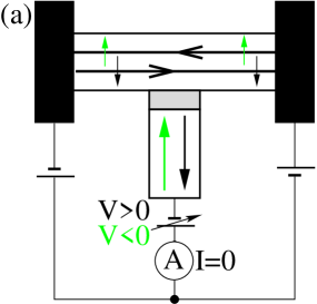
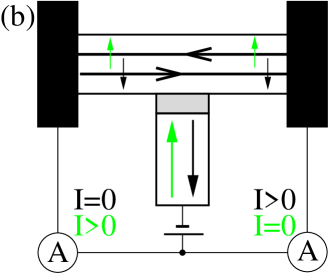
Figure 6: Schematic description of suggested experimental setups for verification of spin accumulation. Panel (a): Measurement of spin–dependent electrochemical potential with ferromagnetic voltage probe. Panel (b): Injection of spin–polarized current via tunnel barrier from ferromagnetic contact, and subsequent measurement of the directionality of current flow probes the chirality of the allowed spin states. Depending on the direction of the magnetization, only one of the two Amperemeters detects a finite current [44].

To obtain linear–transport currents, the scattering problem is solved by standard mode–matching techniques. The usual condition for the probability–current conservation needs to be modified because the velocity operator in the presence of Rashba spin-orbit coupling reads [41, 42]

$$v_{y}=-\frac{i}{\hbar}[y,H_{\mathrm{qw}}]=\hbar(k_{y}+k_{\mathrm{so}}\sigma_{x})/m\quad.$$ (11)

To have a clear understanding of what happens at the interface between a lead without spin–orbit coupling and the wire with spin–orbit coupling, we study first the simple situation of a single interface between a semi–infinite lead and a semi–infinite wire with spin–orbit coupling. The results for the total spin-up(-down) current as a function of the distance from the interface are shown in Fig. 5a. The current flowing in the lead is unpolarized, while in the wire, distant enough from the interface, the current becomes spin–polarized in agreement with the spin properties of the eigenstates shown in Fig. 4a. Hence, the Rashba spin splitting leads to spin accumulation in the wire without ferromagnetic contacts. The other important phenomenon which is apparent from Fig. 5 is the process of current conversion occurring at the interface. This process is mediated by scattering into evanescent modes of the wire, and is possible thanks to the anomalous form of the velocity operator (11). Fig. 4b shows results for the experimentally relevant situation of a finite–length wire with spin–orbit coupling between two leads. Also in this case, we have both spin accumulation and current conversion, plus some finite-size oscillation due to quantum interference [43].

Finally we suggest two possible schemes to enable experimental verification of spin accumulation (see Fig. 6). One possibility would be to weakly couple a ferromagnetic voltage probe to the wire, measuring the chemical potential of the majority spins. Changing the direction of the magnetization of the ferromagnetic contact enables the detection of the difference in chemical potentials of the two spin species. Another possibility could be to use injection of a spin–polarized current from a ferromagnet to probe the chirality of propagating spins in the wire. The direction of current flow should then depend on the direction of the magnetization of the ferromagnet [44].

5 Electron–electron interactions and Rashba spin splitting

Interactions between electrons turn out to have more dramatic consequences in 1D as compared to higher–dimensional systems. Instead of following the familiar [45] Fermi–liquid paradigm, 1D conductors form their own new class of interacting metals dubbed Luttinger liquids [46, 47]. Power–law behavior of electronic correlation functions, such as the tunneling density of states or the momentum–space occupation number, near the Fermi points are a signature of non–Fermi–liquid properties exhibited by interacting 1D systems. Previous work [30] has shown that weak Rashba spin splitting leaves such power laws essentially unaffected. However, the interplay between Luttinger–liquid behavior and spin–orbit coupling turns out to be nontrivial in quantum wires with strong Rashba spin splitting and deserves a more detailed discussion.

The current understanding of interaction effects in 1D systems is based on the possibility to map real systems onto the exactly soluble Tomonaga–Luttinger model [20, 21]. The starting point of such a mapping is linearization of the single–particle dispersion relation near the Fermi points. Furthermore, two chiral electron flavors (right–movers and left–movers) are distinguished according to their velocity direction. In the present case of a strong Rashba–split quantum wire, the spin degeneracy of these chiral electron branches is broken. In the most general case, we can distinguish two right–moving branches having different velocities. As discussed in Sec. 3 above, their spin properties are peculiar because they result from hybridization of quasi–1D subbands with opposite spin. In particular, when Fermi points are sufficiently far away from anticrossings, both right–moving branches can be modeled as having approximately parallel spin. The same is then true for left–movers which, however, have their spin opposite to that of right–movers. To be most general, we do not a priori assign spin labels to the chiral electron branches. Instead, we distinguish them by their different velocities. See Fig. 7 for an illustration.

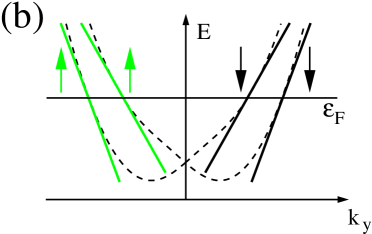
Figure 7: Linearization of the quasi–1D spin–split subband energy dispersion is the starting point for application of the Tomonaga–Luttinger model. (a) In general, we can distinguish two branches of right–movers (R) and left–movers (L) each, labeled A and B here. Their most conspicuous differences are in the magnitude of their Fermi wave numbers and velocities. When Fermi points are located far enough from anticrossings, the situation depicted in (b) arises where electrons from both right–moving branches are in the same spin state. Similarly, left–moving states then turn out to have parallel spin, which is opposite to that of the right–movers

The single–electron part of the Tomonaga–Luttinger Hamiltonian of a quantum wire with strong Rashba spin splitting can then be written as

$$H_{\mathrm{TL}}^{\mathrm{(0)}}=\sum_{\alpha={\mathrm{A,B}}}\sum_{k}\hbar v_{\alpha}k\left(c_{\mathrm{R}\alpha}^{\dagger}c_{\mathrm{R}\alpha}-c_{\mathrm{L}\alpha}^{\dagger}c_{\mathrm{L}\alpha}\right)\quad.$$ (12)

We have omitted uniform shifts of the chemical potential and total energy of the system. Introducing the familiar chiral bosonic phase fields [46, 47] $\phi_{\nu\alpha}$ that are related to the normal–ordered electron density for each branch via $\varrho_{\nu\alpha}=\partial_{x}\phi_{\nu\alpha}/(2\pi)$, with $\alpha=\mathrm{A,B}$ and $\nu=\mathrm{R,L}$, we can write the single–particle and interaction parts of the Tomonaga–Luttinger Hamiltonian $H_{\mathrm{TL}}=H_{\mathrm{TL}}^{\mathrm{(0)}}+H_{\mathrm{TL}}^{\mathrm{(int)}}$ as

$$H_{\mathrm{TL}}^{\mathrm{(0)}} = \frac{\hbar}{4\pi}\int dx\sum_{\nu\alpha}v_{\alpha}\left(\partial_{x}\phi_{\nu\alpha}\right)^{2}\quad,$$ (13)

$$H_{\mathrm{TL}}^{\mathrm{(int)}} = \frac{V_{0}}{8\pi^{2}}\int dx\left(\sum_{\nu\alpha}\partial_{x}\phi_{\nu\alpha}\right)^{2}\quad.$$ (14)

Here we have only included the long–wave–length forward–scattering component $V_{0}$ of the screened Coulomb interaction in the wire. Changing representation to the nonchiral conjugate phase fields $\theta_{\pm}=(\sum_{\nu}\phi_{\nu\mathrm{B}}\pm\sum_{\nu}\phi_{\nu\mathrm{A}})/\sqrt{8\pi}$ and $\Pi_{\pm}=(\partial_{x}\phi_{\mathrm{R}\mathrm{B}}-\partial_{x}\phi_{\mathrm{L}\mathrm{B}}\pm[\partial_{x}\phi_{\mathrm{R}\mathrm{A}}-\partial_{x}\phi_{\mathrm{L}\mathrm{A}}])/\sqrt{8\pi}$, and introducing the abbreviations $v_{+}=(v_{\mathrm{A}}+v_{\mathrm{B}})/2$, $K_{\rho}=\sqrt{1+\frac{2V_{0}}{\pi v_{+}}}$, $v_{\mathrm{pl}}=v_{+}/K_{\rho}$, and $\delta=(v_{\mathrm{B}}-v_{\mathrm{A}})/v_{+}$, we find after some algebra $H_{\mathrm{TL}}=H_{+}+H_{-}+H_{\delta}$, where

$$H_{+} = \frac{\hbar v_{\mathrm{pl}}}{2}\int dx\left\{\frac{1}{K_{\rho}}(\partial_{x}\theta_{+})^{2}+K_{\rho}\,\Pi_{+}^{2}\right\}\quad,$$ (15)

$$H_{-} = \frac{\hbar v_{+}}{2}\int dx\left\{(\partial_{x}\theta_{-})^{2}+\Pi_{-}^{2}\right\}\quad,$$ (16)

$$H_{\delta} = \delta\,\frac{\hbar v_{+}}{2}\int dx\left\{(\partial_{x}\theta_{+})(\partial_{x}\theta_{-})+\Pi_{+}\,\Pi_{-}\right\}\quad.$$ (17)

Comparison with the Tomonaga–Luttinger model Hamiltonian of an ordinary quantum wire [47] shows that $H_{+}$ describes plasmon excitations, i.e., fluctuations in the total electron density of the wire, where $K_{\rho}$ is the usual Luttinger parameter. The term $H_{-}$ represents long–wave–length excitations in the density difference between electrons (both right–moving and left–moving) in the B and A branches, which is unaffected by Coulomb interactions. Note that $\theta_{-}$ and its conjugate field $\Pi_{-}$ do not represent the spin density in the strongly Rashba–split quantum wire — not even in the limit where electrons close to the Fermi points have approximately parallel spin, as depicted in Fig. 7b. Finally, $H_{\delta}$ arises because of the velocity difference for electrons from the A and B branches. Its existence leads to the emergence of four different chiral normal modes that diagonalize $H_{\mathrm{TL}}$, in contrast to the case of an ordinary quantum wire where pairs of left–moving and right–moving normal modes with equal velocities exist that can be combined to two nonchiral normal modes. (The latter represent total–charge and total–spin–density waves, respectively.)

The peculiar spin structure of single–electron states in strongly Rashba–split subbands gives rise to an unusual expression for the Zeeman energy in an external magnetic field $B$. Focusing on the case depicted in Fig. 7b, a straightforward calculation yields

$$H_{\mathrm{Z}}=\frac{g_{\mathrm{e}}\mu_{\mathrm{B}}B}{\sqrt{2\pi}}\int dx\,\,\Pi_{+}\quad,$$ (18)

with electron g–factor $g_{\mathrm{e}}$ and Bohr magneton $\mu_{\mathrm{B}}$.

The above expressions for $H_{\mathrm{TL}}$ and $H_{\mathrm{Z}}$ are quadratic in the bosonic phase fields $\theta_{\pm}$ and their conjugates $\Pi_{\pm}$. Together with the bosonization identities [48] for electrons from each of the chiral branches, it is possible to obtain exact results for electronic correlation functions, which are omitted here because of limited space. In the absence of an external magnetic field, spin–independent correlation functions are identical to those of a two–component Luttinger liquid discussed, e.g., in Refs. [49, 50].

6 Conclusions and outlook

Our study of Rashba spin splitting in low dimensions has given us new insight into the interplay between quantum confinement and spin–orbit coupling. Intriguing spin–dependent transport effects arise in quantum wires having a width that is comparable to the spin–precession length. These could form the basis for realizing spintronics devices without involving any magnetic parts. Possibilities for experimental verification of our predictions have been suggested, which could be realized using present nanofabrication techniques. It will be interesting to investigate, both experimentally and theoretically, spin–orbit effects in related quantum–confined structures such as quantum point contacts and non–semiconductor–based systems.

References

- [1] S. A. Wolf, D. D. Awschalom, R. A. Buhrmann, J. M. Daughton, S. von Molnár, M. L. Roukes, A. Y. Chtchelkanova, D. M. Treger, Science 294 (2001) 1488.
- [2] D. Awschalom, N. Samarth, D. Loss (Eds.), Semiconductor Spintronics and Quantum Computation, Springer Verlag, Berlin, 2002.
- [3] G. A. Prinz, Science 250 (1990) 1092.
- [4] G. A. Prinz, Science 282 (1998) 1660.
- [5] T. Valet, A. Fert, Phys. Rev. B 48 (10) (1993) 7099.
- [6] H. Ohno, Science 281 (5379) (1998) 951.
- [7] E. I. Rashba, Fiz. Tverd. Tela (Leningrad) 2 (1960) 1224 [Sov. Phys. Solid 2 (1960) 1109].
- [8] Y. A. Bychkov, E. I. Rashba, Pis’ma Zh. Éksp. Teor. Fiz. 39 (1984) 66 [JETP Lett. 39 (1984) 78].
- [9] G. Lommer, F. Malcher, U. Rössler, Phys. Rev. Lett. 60 (1988) 728.
- [10] R. Winkler, Phys. Rev. B 62 (2000) 4245.
- [11] J. Nitta, T. Akazaki, H. Takayanagi, T. Enoki, Phys. Rev. Lett. 78 (1997) 1335.
- [12] G. Engels, J. Lange, T. Schäpers, H. Lüth, Phys. Rev. B 55 (1997) R1958.
- [13] S. Datta, B. Das, Appl. Phys. Lett. 56 (1990) 665.
- [14] L. S. Levitov, Y. V. Nazarov, G. M. Eliashberg, Zh. Éksp. Teor. Fiz. 88 (1985) 229 [Sov. Phys. JETP 61 (1985) 133].
- [15] V. M. Edelstein, Solid State Commun. 73 (1990) 233.
- [16] J. Inoue, G. E. Bauer, L. W. Molenkamp, Phys. Rev. B 67 (2003) 033104.
- [17] E. G. Mishchenko, B. I. Halperin, Phys. Rev. B 68 (2003) 045317.
- [18] M. Governale, U. Zülicke, Phys. Rev. B 66 (2002) 073311.
- [19] S. Datta, Electron Transport in Mesoscopic Systems, Cambridge University Press, Cambridge, UK, 1995.
- [20] S. Tomonaga, Prog. Theor. Phys. 5 (1950) 544.
- [21] J. M. Luttinger, J. Math. Phys. 4 (1963) 1154.
- [22] T. Ando, A. B. Fowler, F. Stern, Rev. Mod. Phys. 54 (1982) 437.
- [23] R. Winkler, Spin-Orbit Coupling Effects in Two-Dimensional Electron and Hole Systems, Vol. 191 of Springer Tracts in Modern Physics, Springer, Berlin, 2003.
- [24] E. A. de Andrada e Silva, G. C. La Rocca, F. Bassani, Phys. Rev. B 50 (1994) 8523.
- [25] P. Pfeffer, W. Zawadzki, Phys. Rev. B 52 (1995) R14332.
- [26] E. A. de Andrada e Silva, G. C. L. Rocca, Phys. Rev. B 67 (2003) 165318.
- [27] F. Mireles, G. Kirczenow, Phys. Rev. B 64 (2001) 024426.
- [28] A. V. Moroz, C. H. W. Barnes, Phys. Rev. B 60 (1999) 14272.
- [29] We suspect that the shift of quasi–1D Rashba–split subbands to lower energies, as apparent from Eq. (8), actually prevents the appearance of ‘bumps’ in the dispersion relation that were claimed to exist in Ref. [28]. See Fig. 5c in that paper which shows their numerical results for . For the purpose of direct comparison, we give our numerical results for the same parameter in our Fig. 2b. We find no bumps. Surprisingly, the energies for states at obtained numerically in Ref. [28] are unshifted from the subband–bottom energy at zero , in disagreement with the exact analytical result of our Eq. (8).
- [30] W. Häusler, Phys. Rev. B 63 (2001) 121310(R).
- [31] For a general shape of the confinement potential, mixing is finite between any two subbands with opposite spin, but it is always largest for those adjacent in energy.
- [32] The spin properties of right–movers and left–movers in strong–Rashba–split quantum wires were presented incorrectly in previous works by Moroz and Barnes [33, 34], which has mislead subsequent related studies [35, 36, 37].
- [33] A. V. Moroz, K. V. Samokhin, C. H. W. Barnes, Phys. Rev. Lett. 84 (2000) 4164.
- [34] A. V. Moroz, K. V. Samokhin, C. H. W. Barnes, Phys. Rev. B 62 (2000) 16900.
- [35] A. De Martino, R. Egger, Europhys. Lett. 56 (2001) 570.
- [36] A. Iucci, Phys. Rev B 68 (2003) 075107.
- [37] Y. Yue, Y. Wen, J. Lin, Z. Su, and S. T. Chui,Phys. Rev. B 69 (2004) 153307.
- [38] J. C. Egues, G. Burkard, and D. Loss, Phys. Rev. Lett. 89 (2002) 176401.
- [39] J. C. Egues, G. Burkard, and D. Loss, Appl. Phys. Lett. 82 (2003) 2658.
- [40] G. Feve, W. D. Oliver, M. Aranzana, and Y. Yamamoto, Phys. Rev. B 66 (2002) 155328.
- [41] L. W. Molenkamp, G. Schmidt, and G. E. W.Bauer, Phys. Rev. B 64 (2001) 121202(R).
- [42] U. Zülicke and C. Schroll, Phys. Rev. Lett. 88 (2002) 029701.
- [43] The results shown in Fig. 5 differ from those presented in Fig. 4 of Ref. [18] because, when calculating the latter, the confinement in the leads was taken to be different from that in the wire. (For data shown in Fig. 4 of Ref. [18], the first two subband energies in the leads were and , respectively.) Data shown here are for a uniform confinement potential in the entire structure consisting of the leads and the Rashba–spit wire region. As it turns out, the phenomena of spin–accumulation and current conversion are exhibited for either choice of parameters.
- [44] This detection scheme was suggested to us by F. E. Meijer in a private communication (2003).
- [45] D. Pines, P. Nozières, The Theory of Quantum Liquids, Vol. I, Addison-Wesley, Reading, MA, 1989.
- [46] F. D. M. Haldane, J. Phys. C 14 (1981) 2585.
- [47] J. Voit, Rep. Prog. Phys. 57 (1994) 977.
- [48] J. von Delft, H. Schoeller, Ann. Phys. (Leipzig) 7 (1998) 225.
- [49] K. Penc, J. Sólyom, Phys. Rev. B 47 (11) (1993) 6273.
- [50] T. Kimura, K. Kuroki, H. Aoki, Phys. Rev. B 53 (1996) 9572.