Slow two-level systems in point contacts

Abstract

A great variety of experiments, like heat release measurements, acoustic measurements, and transport measurements on mesoscopic samples have proved that two level systems (TLSs) have a crucial role in the low temperature thermal and electric properties of disordered systems. This paper is aimed at reviewing the role of slow TLSs in point contacts. First the theory of point contacts is summarized, concentrating on the discussion of different point contact models, and on the different regimes of electron flow in the contact, mainly focusing on the ballistic and diffusive limit. The Boltzmann equation is solved in both regimes, and the position dependence of the electrical potential is determined. Then the scattering processes in point contacts are investigated, particularly concentrating on the scattering on slow TLSs. If the the electron assisted transitions between the two states are negligible the electron-two level system interaction can be treated with a simplified Hamiltonian. The scattering on such slow TLSs causes nonlinearity in the current-voltage characteristics of the point contact, which can be determined using Fermi’s golden role. These calculations are presented showing both the contribution of elastic and inelastic scattering, and including the dependence on the position of the TLS, and on the effect of high frequency irradiation. These results are used to discuss the differences between these slow TLSs and the fast centers which may be described by the two channel Kondo model. The available experimental results are analyzed, distinguishing between the effects due to the different types of TLSs.

I INTRODUCTION

In the last decades point contact spectroscopy has been proved to be a very powerful method to study electron-phonon interaction in metals (for reviews see Yanson1986a, ,Jansen, 1980 and Duit, 1989). In the recent years it has been realized that in mesoscopic metallic systems the electron scattering by some dynamical defects may play a major role in understanding the energy relaxation and dephasing processes of the electrons at low temperature (for reviews see Pecs, 2000 and Ujsaghy, 2001). Such defects can also be studied by point contact spectroscopy provided that they are situated in the contact region. These defects can either be magnetic impurities or structural defects where an atom or a group of atoms have a metastable, almost double degenerate groundstate forming a two-level system (TLS). The TLS spectroscopy is very similar to the phonon spectroscopy, but as the TLSs cannot propagate like phonons, they are not in thermal equilibrium with the bath. The TLS can be formed as defects in the bulk region of crystalline materials, or at dislocations, at surfaces due to impurities and also in amorphous materials. In most of the cases the internal structure of the TLSs are unknown and they can behave very differently.

The dynamics of magnetic impurities shows the Kondo effectKondo (1988) where by lowering the temperature a Kondo resonance is developed at the range of the characteristic Kondo temperature, $T_{K}$ and approaching zero temperature a magnetic singlet is formed by the impurity spin and the electrons. In that case near zero temperature the magnetic singlet acts just like a static impurity and the dynamical processes are frozen out.

The subject of slow defects can be described by the conventional theory of TLSs and its application to the point contact is the present review. There are, however, many experimental facts which cannot be described in that way, and show resemblance to the magnetic Kondo anomalies even if their magnetic origin is very unlikely. We make an effort to point at those experiments by comparing the observed behavior with the predictions of the slow TLS model. Several of these are believed to be due to dynamical defects, different from slow TLS. It must be emphasized that there is no theory which is generally accepted and can be applied. Earlier it has been proposed that they are fast TLSs, which can be described by the so called two-channel Kondo model.Vladar1983a ; Vladar1983b ; Vladar1983c That proposal has recently been criticized and debated.Aleiner2001a ; Aleiner2001b ; Ujsaghy (2001); Borda (2003) These scatterers now appear rather as “phantoms” and the present review does not cover that issue, we, however, present the earlier interpretation just to help in reading the earlier experimental publications.

• slow TLS. In that case an atom or a group of atoms can have a transition between the two states of lowest energies by direct tunneling or at higher temperature by thermal excitation over the barrier. In the former case those systems are also called as tunneling centers (for review see Black (1981)). The transition rate can be on the scale of seconds and even on longer scales. In that case e.g. the specific heat may depend on the speed of the measurement as to reach thermal equilibrium takes longer time. The resistivity of such mesoscopic system may jump in time between two or several values on the above time scale, as in small mesoscopic systems the resistivity depends on the position of a single atom even if the two possible atomic positions are much smaller than an atomic distance. The study of point contacts containing TLSs in the contact region turned out to be very powerful as the TLS may result in zero bias anomalies shown by the $I(V)$ characteristics. The electron passing through the point contact can interact dynamically with the TLS or it can be elastically scattered, which scattering depends on the actual position of the atom forming the TLS. The inelastic scattering may result in a back-scattering of the electron in which case the electron does not proceed from one electrode to the other when the applied voltage is larger than the splitting of the TLS and the process shows up as a resistivity minimum at zero bias. In the case of elastic scattering the transmission rate may depend on the position of a single atom and the anomalies can have either sign. The characteristic relaxation times from the TLS causing slow telegraph fluctuation of resistance to those being responsible for zero bias anomalies in the $I(V)$ curve varies over several orders of magnitude, but for all these so-called slow TLSs the average transition time is much longer than the electron-TLS interaction time.

• fast centers. The fast TLSs are strongly debated whether they can show Kondo anomaly.Aleiner2001b ; Ujsaghy (2001); Borda (2003) Here we present the previous ideas just to make contact with the extended literature, and the present status of the problem will be discussed at the end of the paper. If a conduction electron experiences several switching occasions one after the other we speak about fast TLS. These fast TLSs may show Kondo anomaly as the TLS’s two states can be described by a quasi-spin replacing the real impurity spin of the magnetic Kondo problem and the scattered electron can have different spherical momenta e.g. $s$- and $p$-states playing similar role to the real spin of the conduction electron. The spin-flip process of the magnetic Kondo problem is replaced in the latter case by electron assisted transition between the two states of the TLS. That trasnition was is originally believed to be electron assisted tunneling, which is unlikely according to the present theories,Aleiner2001a ; Aleiner2001b however an electron assisted transition without tunneling is still possible.Borda (2003) In point contacts containing magnetic impurities the Kondo resonance scattering contributes to the back-scattering rate, thus the Kondo impurities result in zero bias peak in the dynamical resistivity, which has a width characterized by the Kondo temperature, $T_{K}$. The sign of the peak is just opposite to those caused by slow TLSs. I.K. Yanson and his co-workersYanson1986a ; Lysykh (1980); Omelyanchouk (1980); Naidyuk (1982); Yanson (2001) and also other groupsJansen (1980); Ralph (1983) studied the zero bias anomalies due to intentionally placed magnetic impurities. Considering the Kondo effect there is a significant difference between the magnetic case and the TLS. In the latter case the conduction electrons, additionally to their angular momenta occurring in the Hamiltonian and the coupling, have a further degree of freedom, the real spin, which makes the electronic sea double degenerate although it does not appear in the coupling constants. Referring to that extra degeneracy the phenomenon is called two-channel Kondo problem (2-CK) in contrast to the magnetic one-channel case (1-CK) (for earlier review see Cox, 1999). That extra degeneracy prevents the system to have a singlet ground state at low temperature, it has finite entropy and, therefore, the Fermi liquid behavior does not show up as far as a low energy cutoff (e.g. the energy difference between the two lowest states of the TLS, known as splitting) is reached as the temperature is lowered.

  The condition for the formation of a 2-CK ground state is that the energy splitting is negligible compared to the Kondo temperature, which is generally not expected. The zero bias anomalies have been believed to be powerful tools to make difference between 1-CK and 2-CK problems (for a review see vonDelft, 1998, 1999). For example annealing or electromigration could result in disappearance or modification of the zero bias anomalies in the case of structural defects while such effects are not expected for magnetic impurities.Upadhyay (1997) Similar issues also appear in the electron dephasing time which has been intensively debated recentlyZawadowski (1999); Aleiner2001a ; Aleiner2001b ; Ujsaghy (2001); Imry (1999). Another version of the two-channel Kondo effect was proposed to explain the zero bias anomalies in URu₂Si₂ point contactsRodrigo (1997) where two degenerate localized electron orbitals of the U atom play the role of the TLS which interact with the conduction electrons.Cox (1987, 1999)

The issue of the 2-CK problem was responsible for the great interest in the zero bias anomalies due to TLS and, therefore, it has a great importance to distinguish between anomalies due to slow TLSs and fast scatterers.

Even if a considerable amount of the discussions are carried out considering fast TLSs there is no doubt that in many cases the slow ones are dominant e.g. where the zero bias anomaly in the point contact spectrum has a positive sign.Akimenko (1993); Keijsers (1995, 1998) Working on the issues listed above we learned that the literature on the theory of slow TLSs in point contacts is very much scattered over many papers and journals, the predictions should be collected from a large number of papers, especially, published in Russian and Ukrainian physical journals some of them not available at smaller libraries. That experience encouraged us to collect and at several occasions to complete those results. The present review is written in a self-contained manner, thus no further reading is necessary to follow the theory.

We want to emphasize that the authors did not consider as a task to give the historically proper complete list of references but they picked up those which are the most appropriate ones to get further information.

II Two level systems in solids

II.1 The model of two level systems

The model of two level tunneling systems was at first introduced to explain the unexpected low-temperature behavior of specific heat and thermal conductivity in disordered solids which cannot be described by phonon excitations.Zeller (1971) The model based on two level systems, which was able to explain the linear temperature dependence of specific heat of amorphous dielectrics at low temperatures was suggested by Anderson, Halperin and VarmaAnderson (1972) and Phillips.Phillips (1972) This so-called tunneling model assumes that in an amorphous state some atoms or groups of atoms may switch between two, energetically nearly equivalent configurations. This situation is modeled as a double well potential with two stable states differing by energy $\Delta$, and a potential barrier between them with a tunneling rate $\Delta_{0}$ (see Fig. 1).

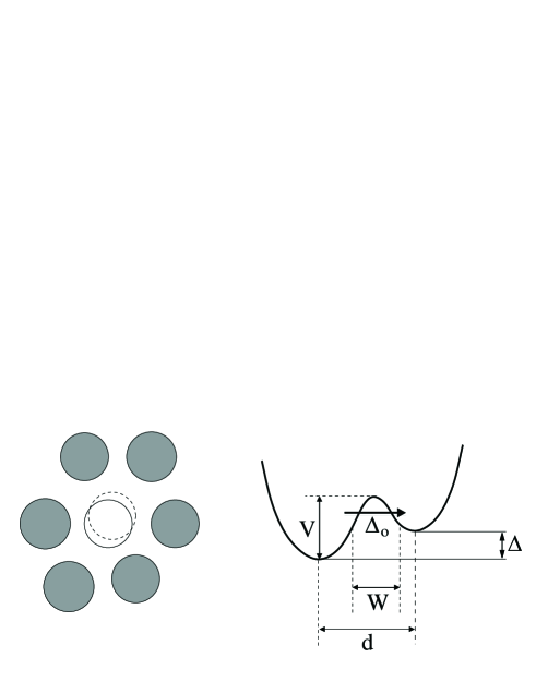
Figure 1: A two-level system is modelled as a double well potential with an energy difference $\Delta$ between the two positions, and a tunneling probability $\Delta_{0}$ for crossing the barrier between the two metastable states. $W$ and $d$ denote the width of the barrier and the distance between the minima, respectively.

The tunneling probability can be approximated in terms of the Gamow parameter ($\lambda$): $\Delta_{0}\sim e^{-\lambda}$, where $\lambda$ is defined by the characteristic height, $V$ and width, $W$ of the potential barrier, and the mass, $M$ of the tunneling particle:

$$\lambda=\sqrt{\frac{2MV}{\hbar^{2}}}W.$$ (1)

Furthermore it is assumed that the TLSs in a solid are uniformly distributed in terms of the parameters $\Delta$ and $\lambda$, that is the density of states $P$ for the first excited states of the TLSs is constant:

$$P(\Delta,\lambda){\rm d}\Delta{\rm d}\lambda=P_{0}{\rm d}\Delta{\rm d}\lambda.$$ (2)

Experimental studies do indeed support this assumption.Hunklinger (1973); Golding (1973); Black (1981)

The two positions of the system are described by a quasispin, and the Hamiltonian of the TLS is expressed in terms of the quasispin’s Pauli-operators:

$$H_{\rm TLS}={1\over 2}\sum\limits_{\alpha,\beta}\left({\Delta b^{+}_{\alpha}\sigma^{z}_{\alpha\beta}b_{\beta}+\Delta_{0}b^{+}_{\alpha}\sigma^{x}_{\alpha\beta}b_{\beta}}\right),$$ (3)

where the indexes $\alpha$ and $\beta$ correspond to the two states of the TLS ($|1\rangle$ and $|2\rangle$), and $b^{+}_{\alpha}$ and $b_{\alpha}$ are the creation and annihilation operators for the state $\alpha$. This Hamiltonian can be diagonalized by writing the eigenstates as:

$$|E_{+}\rangle = \mu|1\rangle+\nu|2\rangle$$

$$|E_{-}\rangle = \nu|1\rangle-\mu|2\rangle.$$ (4)

The eigenenergies are:

$$E_{\pm}=\pm\frac{1}{2}\sqrt{\Delta^{2}+\Delta_{0}^{2}},$$ (5)

and thus the energy splitting between the two eigenstates is:

$$E=\sqrt{\Delta^{2}+\Delta_{0}^{2}}.$$ (6)

The coefficients $\mu$ and $\nu$ can be expressed as:

$$\mu=\frac{E+\Delta}{\sqrt{(E+\Delta)^{2}+\Delta_{0}^{2}}}$$

$$\nu=\frac{\Delta_{0}}{\sqrt{(E+\Delta)^{2}+\Delta_{0}^{2}}}.$$ (7)

For a highly asymmetric TLS, where $\Delta\gg\Delta_{0}$ the energy eigenstates are the two positions of the TLS, that is $\mu=1,0$ and $\nu=0,1$. In the opposite case, where the tunneling energy is much larger than the splitting ($\Delta_{0}\gg\Delta$) the energy eigenstates are delocalized between the two positions, and $\mu=\nu=\frac{1}{\sqrt{2}}$.

II.2 Scattering on two level systems

In a disordered material two level systems are not isolated objects, but they interact with their neighborhood. For instance a strain induced by an elastic wave may change the parameters of the two level systems. It is assumed that only the asymmetry parameter $\Delta$ is influenced by an elastic wave, thus the interaction between two level systems and phonons can be treated as a perturbation in $\Delta$:

$$\delta\Delta=\gamma 2\delta u_{ik},$$ (8)

where $\gamma$ is the coupling constant, and $\delta u_{ik}$ is the appropriate local elastic strain tensor.

In metallic samples the coupling to conduction electrons has to be taken into account as well. The general form of the Hamiltonian describing the interaction between the electrons and the TLS is:Zawadowski1980a ; Zawadowski1980b

$$H_{\rm el-TLS}=\sum\limits_{{\mathbf{p}}_{1},{\mathbf{p}}_{2},\\ \alpha,\beta,\sigma}b^{+}_{\beta}a^{+}_{{\mathbf{p}}_{2}\sigma}V^{\beta\alpha}_{{\mathbf{p}}_{1}{\mathbf{p}}_{2}}a_{{\mathbf{p}}_{1}\sigma}b_{\alpha},$$ (9)

where $a^{+}$ and $a$ are the electron creation and annihilation operators, $\sigma$ is the spin index of the electron and $V$ is the interaction matrix element, which can be decomposed in terms of Pauli operators:Zawadowski1980b

$$V^{\beta\alpha}_{{\mathbf{p}}_{1}{\mathbf{p}}_{2}}=\sum\limits_{i=x,y,z}V^{i}_{{\mathbf{p}}_{1}{\mathbf{p}}_{2}}\sigma^{i}_{\beta\alpha}+V^{0}_{{\mathbf{p}}_{1}{\mathbf{p}}_{2}}\delta_{\beta\alpha}.$$ (10)

The last term stands for potential scattering on the average positioned TLS, the term with $\sigma^{z}$ describes the difference between scattering amplitudes for the two positions of the TLS, while $\sigma^{x}$ and $\sigma^{y}$ correspond to the electron assisted transitions between the two states of the TLS.

II.2.1 Slow two level systems

The interaction Hamiltonian is further simplified if the electron-TLS interaction time is much shorter than the transition time of the TLS, thus the TLS stays in a given position during the electron scattering. For these so-called slow two level systems the electron assisted transitions described by $V^{x}$ and $V^{y}$ can be neglected, and the Hamiltonian is:

$$H_{\rm el-TLS}=\sum\limits_{{\mathbf{p}}_{1},{\mathbf{p}}_{2},\sigma}V^{z}_{{\mathbf{p}}_{1}{\mathbf{p}}_{2}}a^{+}_{{\mathbf{p}}_{2}\sigma}a_{{\mathbf{p}}_{1}\sigma}\cdot\sum\limits_{\alpha,\beta}\sigma^{z}_{\beta\alpha}b^{+}_{\beta}b_{\alpha}+\sum\limits_{{\mathbf{p}}_{1},{\mathbf{p}}_{2},\sigma}V^{0}_{{\mathbf{p}}_{1}{\mathbf{p}}_{2}}a^{+}_{{\mathbf{p}}_{2}\sigma}a_{{\mathbf{p}}_{1}\sigma}\cdot\sum\limits_{\alpha,\beta}\delta_{\beta\alpha}b^{+}_{\beta}b_{\alpha},$$ (11)

the interaction matrix elements between the delocalized energy eigenstates are:

$$\langle E_{-}|H_{\rm el-TLS}|E_{+}\rangle=\sum\limits_{{\mathbf{p}}_{1},{\mathbf{p}}_{2},\sigma}\left[2\mu\nu V^{z}_{{\mathbf{p}}_{2}{\mathbf{p}}_{1}}\right]a_{{\mathbf{p}}_{2}\sigma}^{\dagger}a_{{\mathbf{p}}_{1}\sigma},$$ (12)

which gives the amplitude of the electron’s inelastic scattering on the TLS, which is associated with an energy change, $E$. The matrix elements corresponding to the elastic processes are written as:

$$\langle E_{+}|H_{\rm el-TLS}|E_{+}\rangle = \sum\limits_{{\mathbf{p}}_{1},{\mathbf{p}}_{2},\sigma}\left[V^{0}_{{\mathbf{p}}_{2}{\mathbf{p}}_{1}}+(\mu^{2}-\nu^{2})V^{z}_{{\mathbf{p}}_{2}{\mathbf{p}}_{1}}\right]a_{{\mathbf{p}}_{2}\sigma}^{\dagger}a_{{\mathbf{p}}_{1}\sigma}$$

$$\langle E_{-}|H_{\rm el-TLS}|E_{-}\rangle = \sum\limits_{{\mathbf{p}}_{1},{\mathbf{p}}_{2},\sigma}\left[V^{0}_{{\mathbf{p}}_{2}{\mathbf{p}}_{1}}-(\mu^{2}-\nu^{2})V^{z}_{{\mathbf{p}}_{2}{\mathbf{p}}_{1}}\right]a_{{\mathbf{p}}_{2}\sigma}^{\dagger}a_{{\mathbf{p}}_{1}\sigma}.$$ (13)

In both cases the energy of the scattered electron is conserved, however the scattering cross section is different if the TLS is in the $|E_{+}\rangle$ or $|E_{-}\rangle$ state.

By simple argumentation the interaction strength, $V^{z}$ can be estimated as: $V^{z}\sim(p_{F}d)V$,Black (1979); Vladar1983a as the difference between the electron scattering amplitudes in the two positions must be proportional to the distance of those positions on the scale of the Fermi wavelength, and the strength of the scattering, $V$. $V^{0}$ is very model dependent, e.g. the tunneling atom can be different from the most of the atoms.

II.2.2 Fast two level systems

The electron assisted transition processes are only important in the case of fastly relaxing two level fluctuators. In this case the Hamiltonian given by Eq. (9) can be scaled to the two channel Kondo problem (2CK) with the Hamilton operator:

$$H_{\rm int}=\mbox{\boldmath$\sigma$}_{\rm TLS}V\sum\limits_{p_{1},p_{2},\alpha,\beta,\sigma}a^{+}_{p_{1}\alpha\sigma}\mathbf{S}_{\alpha\beta}a_{p_{2}\beta\sigma},$$ (14)

where the the momentum dependence of $a_{\mathbf{p},\sigma}$ is decomposed into appropriately choosen spherical waves with indices $\alpha,\beta$, and $p=|\mathbf{p}|$ (For details see Vladar1983a, ; Vladar1983b, ). $\mathbf{S}$ is a pseudo-spin corresponding to the spherical indices of the electrons, whereas $\mbox{\boldmath$\sigma$}_{\rm TLS}$ is a pseudo-spin corresponding to the states of the TLS, and $V$ is the interaction strength. In this model the electron spin is an extra degree of freedom compared to the single channel magnetic impurity Kondo problem, and this quantum number is conserved during the interaction and the coupling is independent of that. In contrast to the single-channel Kondo problem, which has a non-degenerated, $S=0$ ground state because of the spin compensation cloud formed by the conduction electrons, the ground state of the two channel Kondo problem has a non-zero entropy. In the two channel Kondo model the conduction electrons overscreen the impurity spin by forming a non-trivial spin state. The low temperature regime of the two channel Kondo model was found to have non-Fermi-liquid behavior.

This paper is devoted to review the literature of the slow TLSs and point contacts. The Kondo regime of the TLSs is out of present consideration, but one can find an up-to-date review of this field in the work of Cox and Zawadowski.Cox (1999)

II.2.3 Scattering rate beyond the Born approximation

In the previous part of this Section the scattering rates due to TLSs are calculated in Born approximation. Considering only the screening interaction $V^{z}$ and ignoring the assisted tunneling rates ($V^{x},V^{y}$) KondoKondo (1984) has found power law correction to the tunneling rate which is due to the building up of a screening cloud or Friedel oscillation around the changed position of the tunneling atom. That is closely related to the Anderson’s orthogonality catastropheAnderson (1967); Kondo (1976, 1988) and the X-ray absorption problem (see e.g. Nozieres, 1969). That phenomenon is associated with creating a large number of electron-hole pairs as the position of the tunneling atom is changed. The renormalized dimensionless coupling constant (usually denoted by $K$) can be expressed in terms of the phase shift $\delta$ describing the scattering of the electrons by the atom in the s-wave channel (see e.g. Yamada, 1985; Kondo, 1988) and the separation distance, $d$ between the two positions of the TLS

$$K=2\left[{1\over\pi}\arctan{{\sqrt{1-a^{2}}\tan\delta}\over{(1+a^{2}\tan^{2}\delta)^{1/2}}}\right]^{2},$$ (15)

where $a=j_{0}(k_{F}d)$ with the spherical Bessel function, $j_{0}$ and $K<1/2$ for only $s$-wave scattering. In the weak coupling limit $\delta\ll 1$ and $k_{F}d\ll 1$ that expression is proportional to $(\varrho_{0}V^{z})^{2}$. In many other publications the notation $\alpha$ is used for $K$ (see e.g. Costi, 1996).

The behavior of a TLS coupled to electronic heat bath (Ohmic region) by the coupling $K$ has been studied in great detail (see e.g. Leggett, 1987 and Weiss, 1999). In general there are two different regions regarding the coupling strength $K$. Here the asymmetry parameter $\Delta$ is disregarded and $T=0$ is taken.

• $0<K<{1\over 2}$ damped coherent oscillation. At $K=0$ the atom has a periodic motion between the two positions. As $K$ is increased the oscillation is more damped and the renormalized tunneling frequency $\Delta_{ren}$ is given by

  $$\Delta_{ren}=\Delta_{0}\left({\Delta_{0}\over{\omega_{c}}}\right)^{K\over{1-K}},$$

  where $\omega_{c}$ is the high frequency cutoff, which has first believed to be the electronic bandwidth (see e.g. Cox, 1999, but according to the adiabatic renormalization it is rather the energy scale of the lower excitations in the potential well where several excited levels are considered.Kagan (1992); Kondo (1988)

• ${1\over 2}<K<1$ incoherent relaxation. The motion is incoherent and the atom is spending longer times in a position before tunneling as $K$ is increased.

Many experimental facts indicate (see next subsection) that the TLSs are in the first region ($K<1/2$) and even can be in the weak coupling limit ($K\ll 1$).

The main issue is how the quasielastic and inelastic scattering rates are modified by the coupling $K$. That problem was investigated by H. Grabert, S. Linkwitz, S. Dattagupta, U. WeissGrabert (1986) considering the neutron scattering by TLS. Those results are very instructive for the present case, there are, however, essential differences:

• Korringa type of relaxations are very important in the relaxation of the TLS coupled to the ohmic electronic heat bath. If energy $\omega$ is transferred to the TLS the spectrum of the TLS is broadened by a relaxation rate proportional to $\omega$. In the case of point contacts that energy may arise from the energy of the electron passing through the point contact. At finite bias, $V$ the system is, however, out of equilibrium and in the stationary state of the TLS the averaged energy of the TLS is proportional to $V$ also. Thus, the nonequlibrium situation should be treated by using e.g. the Keldysh technique.Keldysh (1964)

• The energy transfer is not determined by the applied voltage, in contrast to the neutron scattering experiment where the energy of the incoming and outgoing neutrons are simultaneously measured. In the present case by small change of the voltage the energy of the extra electrons passing through the point contact are given ($\sim V$) but the energy of the scattered electrons is not determined, thus the energy of the outgoing electron shows some distribution. That results in an additional smearing in the spectrum.

In the following we give a brief summary of the neutron scattering case.Grabert (1986) Very accurate results are obtained for low temperature and energies except the range $\omega\ll\Delta_{ren}$. That is certainly the interesting range considering especially for the long range tails of the characteristics which are crucial for the interpretations of the experiments.Keijsers1996a ; Zarand (1998) The calculation was carried out by expanding in the tunneling events and summing up.

More comprehensive studies were performed by using numerical renormalization groupCosti (1996, 1998) for the entire energy range of energy and even including the asymmetry, $\Delta$ and later even for nonequilibrium.Costi (1997).

The previous resultsGrabert (1986) have a very good fit, by the formula

$$S(\omega)\sim{A\over{\exp(kT)-1}}{\omega\over{(\omega-\omega_{0})^{2}+b\omega^{2}}}$$

where $a$, $B$, and $\omega_{0}$ are fitted parameters. That clearly shows a double peak structure with energies $\pm\omega_{0}$. The lines are broadened by a Korringa type energy relaxation rate proportional to $\omega$. In the nearly Lorentzian lineshape no direct role of coupling $K$ was discovered.

Those results are strongly indicating that in weak coupling region that would be very hard to discover any sign of anomalous relaxation rate in the tunneling characteristics. That situation is further complicated by the averaging over the distribution of the energy of the scattered electrons and the out of equilibrium situation. We find, that the experimental studies of the tunneling characteristics are not appropriate tool to look for the interaction effects, except that $\Delta_{0}$ is renormalized. That situation is very different from the cases of one and two channel Kondo impurities, where the characteristics are determined by the Kondo resonances.

II.3 Experimental investigation of two level systems

There are several experimental methods to investigate the kinetics of TLSs. The first two methods to be discussed are studying the TLSs by their interaction with phonons. In heat release measurements the time dependence of heat release or specific heat is measured: after a sudden cool down of the sample due to the energy relaxation of the TLSs it takes a long period of time to reach thermal equilibrium. The second group of measurements investigates the propagation of sound in amorphous materials measuring sound attenuation and sound velocity.Hunklinger (1976)

Heat release measurements basically focus on amorphous dielectrics and superconductors, as in metals the contribution of conduction electrons to the heat capacity usually dominates that of TLSs, thus the estimation of $P_{0}$ is more difficult. According to the heat release measurements of Koláč et al.Kolac (1986) in amorphous metal Fe₈₀B₁₄Si₆ the density of the TLSs is about $P_{0}\approx 1.5\times 10^{44}J^{-1}m^{-3}$.

Though in acoustic measurements basically the phonons are investigated, if the electron - TLS coupling is strong, the results may significantly differ from that on amorphous dielectrics.Golding (1978) A simple description for ultrasound absorption by two level systems is as follows. The occupation numbers for the upper and the lower states of the TLS are $n_{+}$ and $n_{-}=1-n_{+}$, respectively. The probability for ultrasound absorption is $\alpha Pn_{-}$, where $P$ is the ultrasound intensity, and $\alpha$ is the absorption coefficient. The probability of relaxation is $n_{+}/\tau$, where $\tau$ is the relaxation time of the TLS. In balance these two quantities are equal, thus one obtains:

$$n_{-}=\frac{1}{\tau}\frac{1}{\alpha P+\frac{1}{\tau}}.$$ (16)

The absorbed energy is:

$$E_{abs}=\hbar\omega\alpha Pn_{-}=\hbar\omega\frac{\alpha P\frac{1}{\tau}}{\alpha P+\frac{1}{\tau}}.$$ (17)

It is easy to see, that at large enough intensities ($P\to\infty$), the energy absorption saturates to a value inversely proportional to the relaxation time ($E_{abs}\to const./\tau$). In insulators and semiconductors the available maximal ultrasound power is enough to drive the absorption into saturation at $T=1-4$K, but in metals such saturation is only obtained at temperatures as low as $T=10$mK. It implies that the relaxation times in metallic samples are much shorter than in disordered insulators. The interpretation for this experimental observation is, that the electron-TLS scattering processes are dominating in the relaxation of TLSs. Assuming a standard Korringa-like electron - TLS relaxation, where an electron-hole pair is created, at low enough temperatures one obtains:

$$\frac{1}{\tau}\sim KP_{0}kT,$$ (18)

that is, the ultrasound absorption measurements give the opportunity to make an estimation for the electron - TLS coupling parameter ($K$), and the density of the TLSs ($P_{0}$). In fact the acoustic properties of disordered metals do not show universal behavior as in the case of insulating glasses. There are several theoretical approaches (the mentioned standard Korringa-like relaxation,Black (1981) the strong coupling theory of Vladár and Zawadowski,Vladar1983a ; Vladar1983b the electron-polaron effect considered by Kagan and Prokof’evKagan (1988); Kondo (1988)) that may explain the aspects of the relaxation of TLSs due to conduction electrons.Bezuglyi (2000) Still, taking into account the simple electron-TLS coupling given by Eq. (9), the acoustic measurements can give estimations for the density of two level systems ($P_{0}$) or the electron-TLS coupling constant ($K$). In case of superconductors the Korringa relaxation is suppressed by the presence of the superconducting gap, but the gap disappears if a high enough magnetic field is applied on the sample, switching on the TLS-electron interaction.Coppersmith1993a According to the measurements of Esquinazi et al.Esquinazi (1998) in the normal and superconducting state of $Pd_{30}Zr_{70}$ compared with the theory of Kagan and Prokof’evKagan (1988) the coupling parameter is approximately $K\approx 0.4$. The acoustic measurements of Coppersmith and GoldingCoppersmith1993b on the normal conducting amorphous metal Pd_0.775Si_0.165Cu_0.06 estimated the coupling constant as $K\approx 0.2$. For the density of the two level systems a lot of results are available in the literature, and it can be stated generally, that it is the same within a factor of less than 10 over a large variety of disordered material, being metallic glasses or dielectric amorphous material. (For TLSs with energy splitting less than 1 Kelvin it is approximately 1-10ppm.) A detailed review of heat release and acoustic measurements in disordered material can be found in Nittke, 1998; Esquinazi, 1998, and for earlier data see Vladar1983c, .

Electron-TLS interaction can be studied directly by measuring electric transport in disordered metals. Point contact spectroscopy offers the possibility to investigate the properties of even a single two level system centered in the vicinity of the contact. The most spectacular sign of two level systems in point contacts is the so-called telegraph noise: the resistance of the contact is fluctuating between two (or more) discrete values on the timescale of seconds. One can estimate the average lifetimes in the excited ($\tau_{e}$) and ground state ($\tau_{g}$) by recording hundreds of transitions, and fitting the resulting histograms of lifetimes ($P_{e}(t)$ and $P_{g}(t)$) with exponential decay functions ($P_{e}(t)\sim e^{-t/\tau_{e}}$ and $P_{g}(t)\sim e^{-t/\tau_{g}}$, respectively). The two life times are related to each other by the detailed balance, $\tau_{e}/\tau_{g}=e^{-\Delta/k_{b}T}$, where $\Delta$ is the asymmetry parameter. If the TLS jumps to the other state, the electron screening cloud also needs to rearrange, which makes the jumps of the TLS slower. (The building up of the electronic screening cloud is related to a process which is similar to the X-ray absorption in metallic systemsNozieres (1969); Kondo (1988), and which is also called as electron-polaron effect.Kagan (1988, 1992)) From the theoretical point of view this slow-down of the TLS motion is treated as a renormalization of the tunneling amplitude:Kondo (1984)

$$\Delta_{ren}=\Delta_{0}\left(\frac{\Delta_{0}}{\omega_{c}}\right)^{\frac{K}{1-K}},$$ (19)

where $\omega_{c}$ is the bath cutoff frequency for which originally the electron bandwidth had been taken,Kondo (1984) but later it was proposed that it is replaced by a typical energy of the next higher excitation in the potential well.Kagan (1988); Kondo (1988) Golding et al.Golding (1992) studied the two level fluctuation in mesoscopic disordered Bi samples. They argued that their samples were in the strong coupling limit, where the coupling of the TLS to conduction electrons is very strong compared to the tunneling matrix element, thus the latter can be treated as a small perturbation. In this limit the tunneling of the TLS is incoherent, because of the dephasing due to the fast oscillations of the electron bath. Here a theoretical scaling function can be set up: $T^{1-2K}\gamma_{f}=f_{K,\Delta_{0}}(k_{B}T/\Delta)$, which does indeed agree with the experimental result. (The energy splitting of the the TLS can be tuned by changing the electron density, which can be reached by applying weak magnetic field.Zimmerman (1991)) In the limit $k_{B}T/\Delta\gg 1$ the scaling function is constant, i.e. $\gamma_{f}\sim T^{2K-1}$, that is the coupling parameter can be determined from a single fit, giving $K\approx 0.24$ for the particular TLS measured.

The effect of fastly relaxing TLS in point contacts cannot be resolved as a telegraph fluctuation of the resistance, it causes an anomalous behavior in the voltage dependence of the differential resistance around zero bias, a so-called zero bias anomaly (ZBA), which will be a subject of detailed discussion in this review.

III Point contacts

Metallic systems, where two macroscopic electrodes are connected via a contact with small cross section are called “point contacts” (PC) in general, regardless of the actual size of the contact area. It can be generally stated, that the resistance of a point contact is mostly determined by the narrow neighborhood of the junction; therefore, a PC acts as a “microscope” magnifying all kinds of phenomena occurring in the small contact region.

Several methods have been worked out to produce extremely small contacts between two conducting leads. Figure LABEL:4methods presents the four most important experimental techniques. The first one (Fig. LABEL:4methodsa; Muller, 1992) is referred to as mechanically controllable break junction technique (MCBJ). Here the sample (practically a piece of metallic wire) is fixed on the top of a flexible beam, and a small notch is established between the anchoring points. The contact is created in situ at low temperature by breaking the sample with bending the beam, thus one obtains clear and adjustable junction on atomic length scale. The second method (Fig. LABEL:4methodsb; Ralph, 1995) uses nanolithography to establish a small hole in a silicon nitride insulating membrane by etching. If the etching is stopped just when the hole breaks through, the diameter at the bottom edge remains extremely small ($\approx$ 3nm), well below the usual resolution of lithography ($\approx$ 40nm). In the next step metal is evaporated on both sides, creating a high-quality point contact device. This method can provide extremely stable and clear contacts on atomic length scale, however the contact diameter cannot be varied during the measurement. The third drawing (Fig. LABEL:4methodsc) shows a similar arrangement to a scanning-tunneling microscope, a so-called spear-anvil geometry: a vertically movable, sharply tapered needle is pressed onto a flat surface. Finally, Fig. LABEL:4methodsd shows a simple technique, where the edges of two wires are brought into contact. In arrangements (a), (c) and (d) usually a differential screw mechanism is used to adjust the contact supplemented with a piezo-crystal for fine tuning.

The first application of point contacts was carried out by Igor YansonYanson (1974) to investigate electron-phonon scattering in nanojunctions. He found, that the point contact spectrum, obtained as the second derivative of current with respect to the bias voltage ($d^{2}I/dV^{2}$) contains structure due to the electron-phonon interaction described by the Eliashberg function $\alpha^{2}(\omega)F(\omega)$.Khotkevich (1995) This simple method for measuring electron-phonon interaction spectrum became a popular application of PC spectroscopy, however, it can be used to probe other electron scattering processes as well, like electron-TLS interaction, which is the central topic of this paper.

Theoretically, point-contacts are considered as two bulk electrodes connected through a narrow constriction. The simplest, and most commonly used PC model is presented in Fig. LABEL:PCmodels.figa. This so-called opening-like point contact is an orifice with diameter $d$ in an infinite isolating plane between the two electrodes. Another extreme limit is the channel-like PC: a long, narrow neck between the bulk regions with the length being much larger than the diameter, $L\gg d$ (Fig. LABEL:PCmodels.figb). The crossover between the both cases can be obtained by considering the point-contacts as rotational hyperboloids with different opening angles (Fig. LABEL:PCmodels.figc). In most of the cases the shape of the PC does not influence the character of physical processes in the constriction radically, and the main parameter is the ratio of the contact diameter ($d$) and other characteristic length scales in the system. Three fundamental length scales are the mean free paths connected to different scattering processes ($l$); the Fermi wavelength of electrons ($\lambda_{\rm F}$); and the atomic diameter ($d_{\rm at}$).

If the Fermi wavelength or the atomic diameter becomes comparable to the contact size, we speak about quantum point contacts and atomic-sized point contacts, respectively. These systems are reviewed in detail in Agrait, 2003. In this paper we consider contacts, that are neither atomic nor quantum, but that are small enough compared to certain mean free paths, and the calculations are basically performed for an opening type geometry.

Concerning the mean free paths, we have to make difference between the elastic and inelastic scatterings. Under usual experimental conditions the elastic mean free path ($l_{\rm el}$) is smaller than the inelastic one ($l_{\rm in}$). Here the inelastic mean free path is the length of the path an electron travels between two inelastic scatterings ($l_{\rm in=}v_{F}\tau_{\rm in}$). Mostly the important parameter is not $l_{\rm in}$, but the inelastic diffusive length, that is the average distance an electron can diffuse between two inelastic scatterings: $L_{\rm in=}\sqrt{l_{\rm in}l_{\rm el}}$. If the contact diameter is much smaller than any of the mean free paths $d\ll l_{\rm el},l_{\rm in}$, we speak about a ballistic contact. In this case the electron travels through the constriction without any scattering (except for the reflection on the walls). On the other hand, if $d\gg l_{\rm el}$, the electron makes a diffusive motion in the contact, and accordingly we speak about the diffusive regime. At contact diameters exceeding the inelastic diffusive length ($d\gg L_{\rm in}$) the excess energy of the electrons is dissipated inside the constriction, which causes a considerable Joule heating in the contact. This limit is called thermal regime. In the following subsections these different limits are discussed. In many cases the system is characterized by the Knudsen number, $K=d/l_{\rm el}$, which was first introduced for the problem of the gas outflowing from a tank through a hole,Knudsen (1934) but in the recent decades it has been used to characterize point contacts as well.

III.1 Diffusive regime

First the diffusive contacts are treated, for which the electric potential ($\Phi$) can be determined by classical equations. (For a general discussion see Holm, 1967) If the mean free path of the electrons is much shorter than the dimension of the contact ($l_{\rm el}\ll d$) then the current density, $\mathbf{j}$ is given by Ohm’s law in terms of the electric field, $\mathbf{E}$ or the electric potential, $\Phi$:

$$\mathbf{j}=\sigma\mathbf{E}=-\sigma\mbox{\boldmath$\nabla$}\Phi,$$ (20)

where $\sigma$ is the conductivity of the metal. Furthermore due to the charge neutrality in metals the continuity equation holds:

$$\nabla\mathbf{j}=0.$$ (21)

If the conductivity is considered to be constant, these two equations result in the Laplace equation for the electric potential:

$$\triangle\Phi=0.$$ (22)

In this phenomenological approach the scattering processes are included in the conductance, which is inversely proportional to the mean free path, $\sigma\sim l^{-1}$. This treatment does not distinguish between elastic and inelastic electron scattering. In the further treatment of the structures in the dynamical conductance (Sec. IV) the inelastic scatterings play crucial role, therefore, instead of the phenomenological theory the kinetic equations must be used. Here the solution of the Laplace equation is presented in order to determine the linear resistance of a diffusive contact, and to determine the position dependence of the electric potential.

Furthermore, we note that the Laplace equation is only applicable if $\sigma$ is constant is space. This assumption is certainly not valid if the temperature of the contact neighborhood is inhomogeneous, which happens in the thermal regime. This situation is treated in the next subsection. Here we assume that the inelastic diffusive length is much larger than the dimension of the contact, thus the temperature of the contact region is constant.

The Laplace equation should be solved with the boundary conditions:

$$\Phi(z\rightarrow\pm\infty)\rightarrow\mp{V\over 2}.$$ (23)

This problem was first solved by Maxwell.Maxwell (1904) Due to the geometry of the problem the Laplace equation is most easily solved in an elliptical coordinate system demonstrated in Fig. 4 (see e.g. Morse, 1953, Simonyi, 1980).

Figure 4: The adequate elliptical coordinate system, in which the Laplace equation is solved for an opening like point contact.

The transformation between a traditional cylindrical coordinate system $(r,z,\varphi)$ and the elliptical coordinates $(\lambda,\mu,\varphi)$ is determined by the following equations of the ellipses and hyperbolas:

$${r^{2}\over{a^{2}\left(1+\lambda^{2}\right)}}+{z^{2}\over{a^{2}\lambda^{2}}} = 1\qquad{\rm and}$$

$${r^{2}\over{a^{2}\left(1-\mu^{2}\right)}}-{z^{2}\over{a^{2}\mu^{2}}} = 1,$$ (24)

where $a=d/2$ is the radius of the contact; $-\infty\leq\lambda\leq\infty$; and $0\leq\mu\leq 1$. Using Eq. (24) the old coordinates can be expressed in terms of the new ones:

$$r=a\sqrt{\left(1+\lambda^{2}\right)\left(1-\mu^{2}\right)},\qquad\;z=a\lambda\mu.$$ (25)

In this coordinate system the orifice is given by the $\lambda\to 0$ surface, while the isolating layer is defined by $\mu=0$. The next task is to determine the components of the metric tensor in the new coordinates:

$${\rm d}s^{2} = {\rm d}r^{2}+{\rm d}z^{2}+r^{2}{\rm d}\varphi^{2}$$

or, using $\lambda$ and $\mu$,

$${\rm d}s^{2} = a^{2}{{\mu^{2}+\lambda^{2}}\over{1+\lambda^{2}}}{\rm d}\lambda^{2}+a^{2}{{\mu^{2}+\lambda^{2}}\over{1-\mu^{2}}}{\rm d}\mu^{2}+a^{2}\left(1+\lambda^{2}\right)\left(1-\mu^{2}\right){\rm d}\varphi^{2}.$$ (26)

The prefactors are the components of the metric tensor in the new (also orthogonal) coordinate system:

$$g_{\lambda\lambda}=a^{2}{{\mu^{2}+\lambda^{2}}\over{1+\lambda^{2}}},\quad g_{\mu\mu}=a^{2}{{\mu^{2}+\lambda^{2}}\over{1-\mu^{2}}},\quad g_{\varphi\varphi}=a^{2}{\left(1+\lambda^{2}\right)\left(1-\mu^{2}\right)}.$$ (27)

Substituting these into the form of the Laplace operator expressed by the general orthogonal coordinates:

$$\triangle\Phi={1\over\sqrt{g_{11}g_{22}g_{33}}}\left[{\partial\over{\partial x_{1}}}\left(\sqrt{g_{22}g_{33}\over g_{11}}{{\partial\Phi}\over{\partial x_{1}}}\right)+{\partial\over{\partial x_{2}}}\left(\sqrt{g_{11}g_{33}\over g_{22}}{{\partial\Phi}\over{\partial x_{2}}}\right)+{\partial\over{\partial x_{3}}}\left(\sqrt{g_{11}g_{22}\over g_{33}}{{\partial\Phi}\over{\partial x_{3}}}\right)\right],$$ (28)

one can get easily

$$\triangle\Phi={1\over{a^{2}\left(\lambda^{2}+\mu^{2}\right)}}\left[{\partial\over{\partial\lambda}}\left(\left(1+\lambda^{2}\right){{\partial\Phi}\over{\partial\lambda}}\right)+{\partial\over{\partial\mu}}\left(\left(1-\mu^{2}\right){{\partial\Phi}\over{\partial\mu}}\right)+{\partial\over{\partial\varphi}}\left({{\left(\lambda^{2}+\mu^{2}\right)}\over{\left(1+\lambda^{2}\right)\left(1-\mu^{2}\right)}}{{\partial\Phi}\over{\partial\varphi}}\right)\right].$$ (29)

Taking the geometry of the problem into account it is obvious that

$${\partial\Phi\over{\partial\varphi}}=0.$$ (30)

The boundary condition Eq. (23) can only be satisfied if at $\lambda\to\pm\infty$ the potential is independent of $\mu$, that is ${\partial\Phi\over{\partial\mu}}=0$. As an Ansatz we extend this condition to arbitrary $\lambda$ values which means that the equipotential surfaces are the $\lambda={\rm constant}$ surfaces. As these surfaces are orthogonal to the $z=0$ plane it is obvious that electric field has no normal component at the insulating layer. After this consideration the Laplace equation takes the following simple form

$${{\rm d}\over{{\rm d}\lambda}}\left[\left(1+\lambda^{2}\right){{{\rm d}\Phi}\over{{\rm d}\lambda}}\right]=0.$$ (31)

The solution of this equation with the boundary conditions is:

$$\Phi(\lambda)=-{V\over\pi}\arctan(\lambda).$$ (32)

Along the $z$-axis ($\mu=1$), the potential is changing as

$$\Phi(z)=-{V\over\pi}\arctan{z\over a},$$ (33)

which is plotted in Fig. 5.

Figure 5: The potential as a function of the distance measured from the center of the opening type contact along the $z$ axis, in the ballistic and the diffusive limit.

Inside the opening ($\lambda=0$) the electric field has only $z$ component:

$$E_{z}=-{\partial\Phi\over{\partial z}}=-{1\over{a\mu}}{\partial\Phi\over{\partial\lambda}}\bigg{|}_{\lambda=0}={V\over{a\pi}}{1\over{\sqrt{1-({r\over a})^{2}}}}.$$ (34)

It should be noted that the field is the largest at the edge of the opening ($r\to a$) and most of the current flows through that region. The total current flowing through the contact is:

$$I=\sigma\int\limits_{0}^{a}2\pi r{\rm d}r\;E_{z}(r)=2a\sigma V,$$ (35)

and thus the resistance of a diffusive point contact is:

$$R={1\over{\sigma d}}.$$ (36)

This calculation was performed for an opening type contact. In case of a channel type geometry with $L\gg d$ the potential drops in the channel, and the resistance is easily written using Ohm’s law:

$$R=\frac{4L}{\sigma d^{2}\pi}.$$ (37)

III.2 Thermal regime

If the dimension of the contact is larger than the inelastic mean free path, then the electron’s excess energy is dissipated in the contact region, and Joule heating takes place. In this case the contact center can be considerably overheated compared to the bath temperature, and thus the conductivity is also position dependent: $\sigma(T(\mathbf{r}))$. This phenomenon can be treated by considering the equations both for the electrical and the heat conduction. The electrical and thermal current densities are:

$$\mathbf{j}=-\sigma\mbox{\boldmath$\nabla$}\Phi,\quad\mathbf{q}=\kappa\mbox{\boldmath$\nabla$}T,$$ (38)

where $\kappa$ is the heat conductivity and $T$ is the position dependent temperature. The continuity equations for the electrical and thermal current are determined by the charge neutrality and the Joule heating respectively:

$$\nabla\mathbf{j}=0,\quad\nabla\mathbf{q}=-\mathbf{j}\mbox{\boldmath$\nabla$}\Phi.$$ (39)

Furthermore, we assume the validity of the the Wiedemann-Franz law:

$${\kappa\over T}=\mathcal{L}\sigma,$$ (40)

where $\mathcal{L}=(\pi k_{B})^{2}/3e^{2}$ is the Lorentz number. Combining these equations we get:

$$\nabla(\sigma\mbox{\boldmath$\nabla$}\Phi) = 0$$ (41)

$$\frac{\mathcal{L}}{2}\nabla(\sigma\mbox{\boldmath$\nabla$}T^{2})+\sigma(\mbox{\boldmath$\nabla$}\Phi)^{2} = 0.$$ (42)

From these equations it can be easily seen that the temperature is generally related to the electric potential as:

$$T^{2}(\mathbf{r})={\rm const.}-\frac{\Phi^{2}(\mathbf{r})}{\mathcal{L}}.$$ (43)

The constant term is determined by the boundary condition:

$$T(z\to\pm\infty)\to T_{\rm bath},$$ (44)

thus:

$$T^{2}(\mathbf{r})=T^{2}_{\rm bath}+\frac{V^{2}}{4\mathcal{L}}-\frac{\Phi^{2}(\mathbf{r})}{\mathcal{L}}.$$ (45)

In an opening type contact the potential is zero at the contact surface, so the local temperature is written as:

$$T^{2}_{\rm PC}=T^{2}_{\rm bath}+\frac{V^{2}}{4\mathcal{L}},$$ (46)

According to this relation a bias voltage of $100$ mV already heats up a contact from cryogenic temperatures ($\sim 4$ K) to room temperature. This feature has crucial importance in experimental studies. If the measurements are performed on a large contact or at high bias voltages, it can easily happen that the $I(V)$ curve presents the temperature dependence of the conductance instead of the spectroscopic features,Verkin (1979) which will be discussed in Sec. IV.

III.3 Ballistic regime

If the linear dimension of the contact is much smaller than the minimum of the mean free paths the electrons are travelling along straight trajectories, and in the first approximation no scatterings are taken into consideration. This system is described by the equations of semiclassical dynamics, so the space and momentum dependent distribution function, $f_{\mathbf{p}}(\mathbf{r})$ is to be determined beside the electric potential, $\Phi(\textbf{r})$. In this limit the electrons “remember” which side of the contact they are coming from, thus the distribution function at position $\mathbf{r}$ can be expressed as a sum of the terms corresponding to electrons coming from the left or the right side of the contact.Kulik (1978) The distribution function can be determined by solving the homogeneous Boltzmann equation which contains no collision integral:Kulik (1977)

$$\mathbf{v}_{\mathbf{p}}{\partial f_{\mathbf{p}}(\mathbf{r})\over{\partial\mathbf{r}}}-e\mathbf{E}{\partial f_{\mathbf{p}}(\mathbf{r})\over{\partial\mathbf{p}}}=0,$$ (47)

where $\mathbf{E}$ is the electronic field, $\mathbf{E}=-\frac{\partial\Phi(\mathbf{r})}{\partial\mathbf{r}}$, and $\mathbf{v}_{\mathbf{p}}$ is the velocity of the electron with momentum $\mathbf{p}$. Note that the electronic charge $e$ is positive, so the charge of an electron is $-e$. Far from the constriction the boundary condition for the distribution function is that it has to tend to the equilibrium distribution function.

$$\lim_{|\mathbf{r}|\rightarrow\infty}f_{\mathbf{p}}(\mathbf{r})=f_{0}(\varepsilon_{\mathbf{p}}),$$ (48)

where $f_{0}(\varepsilon_{\mathbf{p}})=(e^{\varepsilon_{\mathbf{p}}-\mu\over{kT}}+1)^{-1}$.

If we apply $V$ voltage on the sample, the boundary condition for the potential $\Phi$ takes the form

$$\Phi(z\rightarrow\pm\infty)=\mp{V\over 2}.$$ (49)

The solution of the Boltzmann equation can be found by using the trajectory method.Omelyanchouk (1977) (The trajectories of the electrons are considered to be straight because we are interested in the limit $e|V|/\varepsilon_{\rm F}\ll 1$ and the current we are searching for, depends linearly on the electrical field. It can be shown that the bending of trajectory only contributes to the current in the higher order of the field.) In this way

$$f_{\mathbf{p}}(\mathbf{r})=f_{0}\left(\varepsilon_{\mathbf{p}}+e\int\limits_{-\infty}^{\mathbf{r}}\mathbf{E}{\rm d}\mathbf{l}\right)$$ (50)

holds combined with the charge neutrality condition

$$2e\int{\rm d}^{3}\mathbf{p}\left[{f_{\mathbf{p}}(\mathbf{r})-f_{0}(\varepsilon_{\mathbf{p}})}\right]=0,$$ (51)

where $\int\limits_{-\infty}^{\mathbf{r}}$ denotes the integration over the trajectory of the electron coming from the distant reservoir to the contact region at point $\mathbf{r}$. The distribution function of an electron satisfying the conditions (51), (50) and (48) takes the form in the linear order of the field

$$f_{\mathbf{p}}(\mathbf{r})=f_{0}\left({\varepsilon_{\mathbf{p}}-e\Phi(\mathbf{r})+{eV\over 2}\eta(\mathbf{p},\mathbf{r})}\right),$$ (52)

which is constant along the trajectory as the energy $\varepsilon_{\mathbf{p}}-e\Phi(\mathbf{r})$ is conserved. The expression $eV\eta(\mathbf{p},\mathbf{r})/2$ describes the different value of the chemical potential in the right and left hand sides of the constriction ($\mu=\mu|_{V=0}\pm eV/2$):

$$\eta(\mathbf{p},\mathbf{r})=\cases{+1&for electrons arriving at $\mathbf{r}$ from the left reservoir\cr-1&for electrons arriving at $\mathbf{r}$ from the right reservoir}$$ (53)

(For an illustration see Fig. 6.) That can be also expressed in terms of the solid angle, $\Omega(\mathbf{r})$ at which the opening of the contact is seen from point $\mathbf{r}$:

$$\eta(\mathbf{p},\mathbf{r})=\cases{$sign$(z)&, if $-\mathbf{p}\in\Omega(\mathbf{r})$\cr$-sign$(z)&, if $-\mathbf{p}\not\in\Omega(\mathbf{r})$}.$$ (54)

A simple visualization of the distribution function is presented in Fig. 7.

Figure 6: Different electron trajectories arriving at point $\mathbf{r}$. The values of $\eta(\mathbf{p},\mathbf{r})=\pm 1$ are also indicated.

Figure 7: Visualization of the momentum distribution function at three different points in the case of ballistic limit. The shadowed areas represent the occupied states at function of the direction of the momentum, $\mathbf{p}$. The dashed circle represents the equilibrium Fermi surface in case of completely isotropic distribution. The volume of the shadowed areas are independent of the position $\mathbf{r}$ (charge neutrality).

The potential can be derived by substituting the form (52) of the distribution function into the neutrality condition (51):Omelyanchouk (1977)

$$2e\int{\rm d}^{3}\mathbf{p}\left[{f_{0}\left({\varepsilon_{\mathbf{p}}-e\Phi(\mathbf{r})+{eV\over 2}\eta(\mathbf{p},\mathbf{r})}\right)-f_{0}(\varepsilon_{\mathbf{p}})}\right]=0,$$ (55)

where the integral for equienergetic surfaces is easily expressed by the solid angle $\Omega(\mathbf{r})$, and just an energy integral remains:

$$\int{\rm d}\varepsilon\left[{{\Omega(\mathbf{r})\over 4\pi}f_{0}\left({\varepsilon-e\Phi(\mathbf{r})\pm{eV\over 2}}\right)+\left({1-{\Omega(\mathbf{r})\over 4\pi}}\right)f_{0}\left({\varepsilon-e\Phi(\mathbf{r})\mp{eV\over 2}}\right)-f_{0}(\varepsilon)}\right]=0,$$ (56)

where the upper and lower signs correspond to the cases $z>0$ and $z<0$, respectively. The equation can be solved easily by using the identity

$$\int(f_{0}(\varepsilon+a)-f_{0}(\varepsilon)){\rm d}\varepsilon=-a$$ (57)

for an arbitrary energy shift $a$. We can get the potential in the whole space as:Omelyanchouk (1977)

$$\Phi(\mathbf{r})=-{V\over 2}\left[{1-{{\Omega(\mathbf{r})}\over{2\pi}}}\right]\mathrm{sign}(z).$$ (58)

Here $\Omega(\mathbf{r})$ is the solid angle at which the contact is seen from the position $\mathbf{r}$. The potential depending on the distance measured from the contact along the $z$ axis is shown in Fig. 5 (solid curve).

The current density, $\mathbf{j}$ is determined by the distribution function as follows:

$$\mathbf{j}(\mathbf{r})=-2e\int\frac{{\rm d}^{3}\mathbf{p}}{(2\pi)^{3}}{\mathbf{v}_{\mathbf{p}}f_{\mathbf{p}}(\mathbf{r})}.$$ (59)

The current through the contact is calculated by integrating the $z$-component of the current density over the area of the contact, $A$:

$$I=\int\limits_{A}{\rm d}A\;j_{z}(z=0),$$ (60)

At the contact surface half of the electrons go to the left with a distribution function $f_{0}(\varepsilon-eV/2)$ and half of the electrons goes to the right with a distribution function $f_{0}(\varepsilon+eV/2)$, thus the current is written as

$$I=-e\int\limits_{A}{\rm d}A\int\limits_{\varepsilon_{\mathbf{p}}=\varepsilon}\frac{{\rm d}S_{\varepsilon}}{(2\pi)^{3}}\int{\rm d}\varepsilon\frac{|v_{z}|}{\hbar|\mathbf{v_{\mathbf{p}}}|}\left(f_{0}(\varepsilon+\frac{eV}{2})-f_{0}(\varepsilon-\frac{eV}{2})\right),$$ (61)

where the integral $\int{\rm d}S_{\varepsilon}$ is taken over an equienergetic surface in the $\mathbf{p}$-space. At low enough temperature and voltage ($k_{\rm B}T\ll\varepsilon_{\rm F}$ and $eV\ll\varepsilon_{\rm F}$) the expression $\int({f_{0}(\varepsilon+{eV\over 2})-f_{0}(\varepsilon-{eV\over 2})}){\rm d}\varepsilon$ equals $eV$ according to the identity (57), so the current is written as:

$$I=\frac{e^{2}AS_{\rm F}}{\hbar(2\pi)^{3}}\langle\cos(\vartheta)\rangle_{\rm FS}\cdot V,$$ (62)

where $A$ is the area of the contact, $S_{\rm F}$ is the area of the Fermi surface, $\cos\vartheta=v_{z}/v_{\rm F}$ and $\langle{...}\rangle_{\rm FS}=\int{\rm d}S_{\rm F}(...)/S_{\rm F}$ denotes the average taken over the Fermi surface. The conductance of a ballistic point-contact given by the formula (62) is known as the Sharvin conductance.Sharvin (1965) For free electron gas the Sharvin conductance is simplified as:

$$G_{\rm S}=\frac{2e^{2}}{h}\left(\frac{k_{\rm F}d}{4}\right)^{2}.$$ (63)

III.4 Intermediate case between the ballistic and diffusive limit

In the intermediate region between the diffusive and ballistic regime an interpolating formula can be set up by numerically solving the Boltzmann equation for arbitrary ratio of the contact diameter and mean free path, $l$:Wexler (1966)

$$R=l/d\cdot\frac{16}{3\pi\sigma d}+\Gamma(l/d)\frac{1}{\sigma d},$$ (64)

where $\Gamma(l/d)$ is a numerically determinable monotonous function, $\Gamma(0)=1$; $\Gamma(\infty)=0.694$. Note that the first term is exactly the Sharvin resistance by putting the Drude resistivity into the formula, $\rho=mv_{F}/le^{2}n$, thus it is actually independent of $l$. This formula provides the possibility to estimate the contact diameter from the contact resistance.

IV Scattering on slow TLSs in point contacts.

The voltage applied on a point contact results in a nonequilibrium distribution of the conduction electrons in the contact region. An electron coming from the right reservoir has an energy larger by $eV$ than those coming from the left reservoir. This energy can be released through inelastic scattering processes, which can happen in such a way that an electron that has already crossed the contact is scattered back through the opening. This so-called backscattering reduces the current, thus the energy dependence of the scattering probability can be traced by measuring the nonlinearity of the current as the bias voltage is varied. This phenomenon was first used by Igor YansonYanson (1974) (for a review see Yanson1986a, ) to study the phonon spectra and the electron-phonon interaction and since that it is widely applied.

In this section we discuss the nonlinearities in the current voltage characteristics due to the scattering on slow TLSs, which show strong similarities to localized phonons. There is, however, an essential difference between the two cases, while the phonons contribute to the voltage region up to $30$ meV, the TLSs manifest themselves below or even well below $1$ meV due to their characteristic energies. The main contribution to the $I(V)$ characteristics comes from the close region of the contact, therefore a microscopic process like a transition of one atom from one position to another in the contact region occurs as a significant measurable change in the current. Considering the TLSs the main advantage of the point contact spectroscopy is that in case of small enough contacts one can investigate just one or few scattering centers.

The current through the contact can be derived by solving the classical stationary Boltzmann equation

$$\mathbf{v}_{\mathbf{p}}{{\partial f_{\mathbf{p}}(\mathbf{r})}\over{\partial\mathbf{r}}}-e\mathbf{E}{{\partial f_{\mathbf{p}}(\mathbf{r})}\over{\partial\mathbf{p}}}=I(\mathbf{p},\mathbf{r}),$$ (65)

where $I(\mathbf{p},\mathbf{r})$ is the collision integral for the electron with momentum $\mathbf{p}$ at position $\mathbf{r}$, which is assumed to be local in real space.

In the case of bulk phonons the collision integral is

$$I_{\rm ph}(\mathbf{p},\mathbf{r}) = \sum\limits_{\alpha}\int{\rm d}^{3}\mathbf{q}\;W_{\mathbf{q}}^{\alpha}\Bigg{\{}\left[f_{{\mathbf{p}}+{\mathbf{q}}}(1-f_{\mathbf{p}})(N_{\mathbf{q}}^{\alpha}+1)-f_{\mathbf{p}}(1-f_{{\mathbf{p}}+{\mathbf{q}}})N_{\mathbf{q}}^{\alpha}\right]\delta(\varepsilon_{{\mathbf{p}}+{\mathbf{q}}}-\varepsilon_{\mathbf{p}}-\omega_{\mathbf{q}}^{\alpha})+$$ (66)

$$\left[f_{{\mathbf{p}}-{\mathbf{q}}}(1-f_{\mathbf{p}})N_{\mathbf{q}}^{\alpha}-f_{\mathbf{p}}(1-f_{{\mathbf{p}}-{\mathbf{q}}})(N_{\mathbf{q}}^{\alpha}+1)\right]\delta(\varepsilon_{{\mathbf{p}}-{\mathbf{q}}}-\varepsilon_{\mathbf{p}}-\omega_{\mathbf{q}}^{\alpha})\Bigg{\}},$$

where $W_{\mathbf{q}}$ is proportional to the squared matrix element of the electron-phonon coupling, $N_{\mathbf{q}}^{\alpha}$ is the phonon occupation number for momentum ${\mathbf{q}}$ and energy $\omega_{\mathbf{q}}$ in phonon branch $\alpha$. There is another term of the collision integral which is due to the elastic (impurity) scattering but that is not given here. The collision integral vanishes far from the point contact because well inside the electrodes thermal equilibrium exists. The situation is further simplified when the following assumptions are valid: (i) the electron-phonon interaction is homogeneous in the real space; (ii) the phonon distribution corresponds to thermal equilibrium. In that case the information on the contact geometry and also the elastic scattering due to impurities in the dirty limit can be expressed by a geometrical factor $K(\mathbf{p},\mathbf{p}^{\prime})$ in the expression of the current which depends only on the momenta $\mathbf{p}$ and $\mathbf{p}^{\prime}$ of the incoming and outgoing electrons. That factor is frequently called as the $K$-factor (see e.g. Kulik, 1981; Ashraf, 1982). In the case of phonons the $K$-factor for a ballistic opening like contact is written as:

$$K(\mathbf{p},\mathbf{p}^{\prime})=\frac{|\hat{p}_{z}\hat{p}_{z}^{\prime}|}{|\hat{p}_{z}^{\prime}\hat{\mathbf{p}}-\hat{p}_{z}\hat{\mathbf{p}}^{\prime}|}\Theta(-\hat{p}_{z}\hat{p}_{z}^{\prime}),$$ (67)

where $\hat{\mathbf{p}}$ $\hat{\mathbf{p}}^{\prime}$ are the unit vector parallel with $\mathbf{p}$ and $\mathbf{p}^{\prime}$, while $\hat{p}_{z}$ and $\hat{p}_{z}^{\prime}$ are the $z$ components of these unit vectors, where the $z$ direction is the axis of the contact. The $K$-factor can be also calculated for a diffusive contact:

$$K(\mathbf{p},\mathbf{p}^{\prime})=\frac{9\pi}{32}\frac{l_{\rm el}}{d}(\hat{p}_{z}^{2}-\hat{p}_{z}^{\prime 2}),$$ (68)

where $l_{\rm el}$ is the elastic mean free path, and $d$ is the contact diameter.

At zero temperature the logarithmic derivative of the resistance can be expressed by a function $G(\omega)=\tilde{\alpha}^{2}(\omega)F(\omega)$, where $F(\omega)$ is the density of states of phonons and $\alpha(\omega)$ is the modified electron-phonon coupling which contains the $K$-factor. Without that factor it is just the electron-phonon coupling strength and in that case $G(\omega)$ is the Eliashberg function known in the theory of superconductivity. The main result is

$${1\over R}{dR\over{dV}}\sim G({eV\over\hbar}).$$ (69)

In case of single crystals $G(\omega)$ depends also on the orientation of the crystal, which makes it possible to study the anisotropy of the phonon spectrum.Yanson1986a Measuring ${1\over R}{dR\over{dV}}$ the phonon spectra were determined for many different cases and the structures in them were identified as the details of the spectra.Khotkevich (1995) Those structures, however, are superimposed on a continuous background.

Until now, it is assumed that the phonons are in thermal equilibrium, which is the correct assumption as far as the phonons at the contact region arrive from a large distance without any collision where the thermal bulk distribution is realized. That is, however, not the case when in the contact region the phonon mean free path is comparable with the contact size. Then the phonons generated by the non-equilibrium electrons in the contact region cannot escape thus the phonons are also out of equilibrium. The measure of non-equilibrium is limited by the energy relaxation time of the phonons $\tau_{\rm ph}$. The non-equilibrium localized phonons contribute to the background resistance.vanGelder (1978, 1980); Jansen (1980) That can be studied by measuring the amplitude of the background as a function of the frequency of the applied voltageKulik (1985); Yanson (1985); Balkashin (1992) and at high frequency ($\omega\tau_{\rm ph}\gg 1$) that is decreasing. These phenomena will be studied in the context of scattering on TLSs as well.

IV.1 Scattering on TLSs in a ballistic contact

In the following the Boltzmann equation will be solved considering only the electron-TLS interaction. It will be assumed that the density of the TLSs is low thus an electron scatters only once in the orifice region and the contribution of the different TLSs are additive. First the ballistic limit is treated, where both the elastic and inelastic mean free paths are larger than the size of the contact.

The collision term related to a single TLS is very similar to the case of phonons, the momentum is, however, not conserved. Furthermore, the TLS has only two states with population $n_{+}$ and $n_{-}$ ($n_{+}+n_{-}=1$) corresponding to the TLS energy levels $E_{+}$ and $E_{-}$ (see Sec. II). The situation is different from those cases of phonons, where the phonon mean free path is large compared to the size of orifice, $l_{\rm ph}\gg d$ and the phonon distribution is the bulk one which is in thermal equilibrium with the contact regions. In the case of TLSs the interaction is localized in space, thus the TLSs in the contact region are decoupled from the bulk region and they can be considerably out of thermal equilibrium due to the voltage drop at the contact. Therefore, the situation is similar to the special case of localized phonons with $l_{\rm ph}\leq d$ shortly discussed in the introductory remarks of this section.

The collision term similar to Eq. (66) can be written as the sum of inelastic and elastic terms as $I_{{\mathbf{R}},\rm TLS}(\mathbf{p},\mathbf{r})=I_{{\mathbf{R}},\rm TLS,in}(\mathbf{p},\mathbf{r})+I_{{\mathbf{R}},\rm TLS,el}(\mathbf{p},\mathbf{r})$. In the inelastic case the TLS jumps to its other state due to the scattering, and thus the energy of the electron changes by $E=E_{+}-E_{-}$. The strength of the interaction is characterized by $W_{\mathbf{p}\mathbf{p}^{\prime}}$, which is obtained from the interaction matrix elements (Eq. 12) by Fermi’s golden rule as

$$W_{\mathbf{p}\mathbf{p}^{\prime}}=\frac{2\pi}{\hbar}\left|\langle\mathbf{p},E_{+}|H_{\rm e-TLS}|\mathbf{p}^{\prime},E_{-}\rangle\right|^{2}=\frac{2\pi}{\hbar}\left|\langle\mathbf{p},E_{-}|H_{\rm e-TLS}|\mathbf{p},^{\prime}E_{+}\rangle\right|^{2}=\frac{2\pi}{\hbar}\left|2\mu\nu V^{z}_{\mathbf{p}\mathbf{p}^{\prime}}\right|^{2}.$$ (70)

The interaction strength is symmetric in the incoming and outgoing momentum, and in the neighborhood of the Fermi surface it depends only on the unit vectors $\hat{\mathbf{p}}$ and $\hat{\mathbf{p}}^{\prime}$, i.e. $W_{\mathbf{p}\mathbf{p}^{\prime}}=W_{\hat{\mathbf{p}}\hat{\mathbf{p}}^{\prime}}=W_{\hat{\mathbf{p}}^{\prime}\hat{\mathbf{p}}}$. The collision integral for the inelastic scattering is written as:

$$I_{{\mathbf{R}},\rm TLS,in}(\mathbf{p},\mathbf{r}) \simeq \delta(\mathbf{r}-\mathbf{R})\int{{\rm d}^{3}\mathbf{p}^{\prime}\over{(2\pi\hbar)^{3}}}W_{\mathbf{p}\mathbf{p}^{\prime}}\times$$ (71)

$$\Bigg{\{}f_{{\mathbf{p}}^{\prime}}(1-f_{\mathbf{p}})n_{-}\delta(\varepsilon_{{\mathbf{p}}^{\prime}}-\varepsilon_{{\mathbf{p}}}-E)+f_{{\mathbf{p}}^{\prime}}(1-f_{\mathbf{p}})n_{+}\delta(\varepsilon_{{\mathbf{p}}^{\prime}}-\varepsilon_{{\mathbf{p}}}+E)$$

$$-f_{{\mathbf{p}}}(1-f_{{\mathbf{p}}^{\prime}})n_{-}\delta(\varepsilon_{{\mathbf{p}}}-\varepsilon_{{\mathbf{p}}^{\prime}}-E)-f_{{\mathbf{p}}}(1-f_{{\mathbf{p}}^{\prime}})n_{+}\delta(\varepsilon_{{\mathbf{p}}}-\varepsilon_{{\mathbf{p}}^{\prime}}+E)\Bigg{\}},$$

where $\mathbf{R}$ is the place of the TLS.

The current correction due to the elastic scattering processes can be written similarly with two remarks: (i) in an elastic process the energy of the TLS does not change, thus $E=0$ must be inserted; (ii) the scattering cross section is different for the TLS being in the “$+$” and the “$-$” state. According to the matrix elements in Eq. (13), the two scattering strengths are given as:

$$W^{+}_{\hat{\mathbf{p}}\hat{\mathbf{p}}^{\prime}} = \frac{2\pi}{\hbar}\left|\langle\mathbf{p},E_{+}|H_{\rm e-TLS}|\mathbf{p}^{\prime},E_{+}\rangle\right|^{2}=\frac{2\pi}{\hbar}\left|V^{0}_{{\mathbf{p}}{\mathbf{p}^{\prime}}}+(\mu^{2}-\nu^{2})V^{z}_{{\mathbf{p}}{\mathbf{p}^{\prime}}}\right|^{2}$$

$$W^{-}_{\hat{\mathbf{p}}\hat{\mathbf{p}}^{\prime}} = \frac{2\pi}{\hbar}\left|\langle\mathbf{p},E_{-}|H_{\rm e-TLS}|\mathbf{p}^{\prime},E_{-}\rangle\right|^{2}=\frac{2\pi}{\hbar}\left|V^{0}_{{\mathbf{p}}{\mathbf{p}^{\prime}}}-(\mu^{2}-\nu^{2})V^{z}_{{\mathbf{p}}{\mathbf{p}^{\prime}}}\right|^{2}.$$ (72)

After introducing these notations the correction to the collision integral for the elastic scattering is:

$$I_{\mathbf{R},\rm TLS,el}(\mathbf{p},\mathbf{r}) \simeq \delta(\mathbf{r}-\mathbf{R})\int{{\rm d}^{3}\mathbf{p}^{\prime}\over{(2\pi\hbar)^{3}}}\left(W^{+}_{\hat{\mathbf{p}}\hat{\mathbf{p}}^{\prime}}n_{+}+W^{-}_{\hat{\mathbf{p}}\hat{\mathbf{p}}^{\prime}}n_{-}\right)\left[f_{{\mathbf{p}}^{\prime}}(1-f_{\mathbf{p}})-f_{{\mathbf{p}}}(1-f_{{\mathbf{p}}^{\prime}})\right]\delta(\varepsilon_{{\mathbf{p}}}-\varepsilon_{{\mathbf{p}}^{\prime}}).$$ (73)

The electron distribution function $f_{\mathbf{p}}(\mathbf{r})$ and the electric potential is expanded in terms of $d/l_{\rm in}$. At a large distance measured from the orifice the potential is constant and $\lim_{|{\mathbf{r}}|\to\infty}\Phi(\mathbf{r})=\pm V/2$. Thus, at $|{\mathbf{r}}|\gg l_{\rm in}$ the electrons are in thermal equilibrium. The distribution function $f_{\mathbf{p}}(\mathbf{r})$ and the potential $\Phi(\mathbf{r})$ can be expanded as

$$f_{\mathbf{p}}(\mathbf{r}) = f_{\mathbf{p}}^{(0)}(\mathbf{r})+f_{\mathbf{p}}^{(1)}(\mathbf{r})+\dots$$

$$\Phi(\mathbf{r}) = \Phi^{(0)}(\mathbf{r})+\Phi^{(1)}(\mathbf{r})+\dots,$$ (74)

and similarly the electric field

$$\mathbf{E}(\mathbf{r})=\mathbf{E}^{(0)}(\mathbf{r})+\mathbf{E}^{(1)}(\mathbf{r})+\dots,$$ (75)

where the upper indices $(0)$, $(1)$ label the order in the strength of the electron-TLS coupling. The zero order terms have been previously calculated and the following treatment is restricted to the first order terms. The previous results are

$$f_{\mathbf{p}}^{(0)}(\mathbf{r})=f_{0}\left(\varepsilon_{\mathbf{p}}-e\Phi(\mathbf{r})+{eV\over 2}\eta(\mathbf{p},\mathbf{r})\right),$$ (76)

and according to Eq. (58)

$$\Phi^{(0)}(\mathbf{r})=-{V\over 2}\left(1-{\Omega(\mathbf{r})\over{2\pi}}\right){\rm sign}(z),$$ (77)

for a round orifice perpendicular to the $z$-axis, where $f_{0}$ is the Fermi function. The first order terms in the Boltzmann equation given by Eq. (65) can be written as

$$\mathbf{v}_{\mathbf{p}}{\partial f_{\mathbf{p}}^{(1)}(\mathbf{r})\over{\partial\mathbf{r}}}-e\mathbf{E}^{(0)}(\mathbf{r}){\partial f_{\mathbf{p}}^{(1)}(\mathbf{r})\over{\partial\mathbf{p}}}=e\mathbf{E}^{(1)}(\mathbf{r}){\partial f_{\mathbf{p}}^{(0)}(\mathbf{r})\over{\partial\mathbf{p}}}+I_{\rm coll}^{(0)}(\mathbf{p},\mathbf{r}),$$ (78)

where the label $(0)$ of the collision term indicates that the collisions are calculated with the distribution functions of zeroth order, $f^{(0)}$.

The change in the potential is determined again by the neutrality condition given by Eq. (51) for $f^{(0)}$, which is

$$-e\int{{\rm d}^{3}\mathbf{p}\over{(2\pi\hbar)^{3}}}f_{\mathbf{p}}^{(1)}(\mathbf{r})=0.$$ (79)

The boundary conditions are

$$\lim_{|\mathbf{r}|\to\infty}f_{\mathbf{p}}^{(1)}(\mathbf{r})=0,$$ (80)

and

$$\lim_{|\mathbf{r}|\to\infty}\Phi^{(1)}(\mathbf{r})=0.$$ (81)

In order to determine $f^{(1)}$ and $\Phi^{(1)}$ the trajectory method is used (see e.g. Jansen, 1980) dealing with phonons. Electron trajectories are considered where the electron comes from the left or right and arrives to the plane of the orifice at time $\tau=0$ at point $\mathbf{r}$ with momentum $\mathbf{p}$ to calculate the current flowing through the orifice. These trajectories correspond to zeroth order. Moving along the trajectory $\mathbf{r}(\tau),\mathbf{p}(\tau)$ the distribution function varies as

$${\partial f^{(1)}(\mathbf{p}(\tau),\mathbf{r}(\tau))\over{\partial\tau}}={\partial\mathbf{p}(\tau)\over{\partial\tau}}{\partial f^{(1)}(\mathbf{p}(\tau),\mathbf{r}(\tau))\over{\partial\mathbf{p}(\tau)}}+{\partial\mathbf{r}(\tau)\over{\partial\tau}}{\partial f^{(1)}(\mathbf{p}(\tau),\mathbf{r}(\tau))\over{\partial\mathbf{r}(\tau)}},$$ (82)

where ${\partial\mathbf{p}(\tau)\over{\partial\tau}}=-e\mathbf{E}$, and ${\partial\mathbf{r}(\tau)\over{\partial\tau}}=\mathbf{v}_{\mathbf{p}}$. This equation can be integrated and using the Boltzmann equation one finds for $f^{(1)}$ at $\tau=0$

$$f^{(1)}(\mathbf{p},\mathbf{r})=\int\limits_{-\infty}^{0}{\rm d}\tau\Big{\{}-e{{\rm d}\Phi^{(1)}(\mathbf{r}(\tau))\over{{\rm d}\mathbf{r}}}{\partial f^{(0)}(\mathbf{p}(\tau),\mathbf{r}(\tau))\over{\partial\mathbf{p}(\tau)}}+I_{\rm coll}^{(0)}(\mathbf{p}(\tau),\mathbf{r}(\tau))\Big{\}}.$$ (83)

Here the collision term describes the adding or taking off electrons to the trajectory arriving at the contact at $\tau=0$. In the expression of $f^{(1)}$ only the terms linear in the voltage are kept, thus ${\partial f^{(0)}(\mathbf{p}(\tau),\mathbf{r}(\tau))\over{\partial\mathbf{p}(\tau)}}$ in the above equation can be approximated by the zeroth order term $\mathbf{v}_{\mathbf{p}}{\partial f_{0}\over{\partial\varepsilon_{\mathbf{p}}}}$. Taking into account that ${\rm d}\mathbf{r}=\mathbf{v}_{\mathbf{p}}{\rm d}\tau$ the first term of the integral can be performed, thus

$$f^{(1)}(\mathbf{p},\mathbf{r})=-e\Phi^{(1)}(\mathbf{r}){\partial f_{0}\over{\partial\varepsilon_{\mathbf{p}}}}+\int\limits_{-\infty}^{0}{\rm d}\tau\;I_{\rm coll}^{(0)}(\mathbf{p}(\tau),\mathbf{r}(\tau)).$$ (84)

The equation of electrical neutrality taken at $\tau=0$ with $\mathbf{p}(\tau=0)=\mathbf{p}$ and $\mathbf{r}(\tau=0)=\mathbf{r}$ combined with the equation above determines $\Phi^{(1)}(\mathbf{r})$

$$e\Phi^{(1)}(\mathbf{r})={\int{{\rm d}^{3}\mathbf{p}\over{(2\pi\hbar)^{3}}}\int\limits_{-\infty}^{0}{\rm d}\tau\;I_{\rm coll}^{(0)}(\mathbf{p}(\tau),\mathbf{r}(\tau))\over{\int{{\rm d}^{3}\mathbf{p}\over{(2\pi\hbar)^{3}}}{\partial f_{0}\over{\partial\varepsilon_{\mathbf{p}}}}}}.$$ (85)

The general expression of the electrical current flowing through the surface of the contact is

$$I=-2e\int{\rm d}^{2}\varrho\int{{\rm d}^{3}\mathbf{p}\over{(2\pi\hbar)^{3}}}v_{\mathbf{p}}^{z}f(\mathbf{p},\mathbf{r}),$$ (86)

where ${\rm d}^{2}\varrho$ is the surface element of the contact and the integral is taken over the orifice, the factor $2$ is due to the electron spin. The change $\delta I$ in the total current due to the presence of the TLS can be separated as

$$I(V)=I_{0}(V)+\delta I(V),$$

and $\delta I(V)$ can be further split, whether the electron scattering is elastic or inelastic

$$\delta I(V)=\delta I_{\rm el}+\delta I_{\rm in}.$$

Making use of the expression (84) for $f^{(1)}$ only the collision term contributes to the current because the other term is even in the momentum. The integral according to the time can be transformed to the one along the path using ${\rm d}\tau={{\rm d}s\over{v_{\mathbf{p}}}}$ where ${\rm d}s$ is the element of the path. The expression for the change of the current due to the presence of collision on TLS is

$$\delta I=-2e\int{\rm d}^{2}\varrho\int{{\rm d}^{3}\mathbf{p}\over{(2\pi\hbar)^{3}}}v_{\mathbf{p}}^{z}\int\limits_{-\infty}^{0}{{\rm d}s\over{v_{\mathbf{p}}}}I_{\rm coll}^{(0)}(\mathbf{p}(\tau),\mathbf{r}(\tau)).$$ (87)

The path of the integral is changed due to the collisions but it may contain reflections by the insulating surface of the contact. The next step is to introduce the collision term due to a single TLS at position $\mathbf{R}$, given by Eq. (71). As the paths arriving at the surface element of the orifice ${\rm d}^{2}\varrho$ are straight lines, the volume element for the scattering event is ${\rm d}^{3}\mathbf{r}={\rm d}^{2}\varrho{\rm d}s\cos\theta$ where $\theta$ is the angle between the path and $z$ direction. Now the integration over different paths and position of the collision gives

$$\delta I_{\mathbf{R}}=-2e\int\limits_{\Omega_{\mathbf{R}}}{{\rm d}^{3}\mathbf{p}\over{(2\pi\hbar)^{3}}}{v_{\mathbf{p}}^{z}\over{v_{\mathbf{p}}}}\cos\theta\cdot I_{{\mathbf{R}},\rm TLS}(\mathbf{p})$$ (88)

where $I_{{\mathbf{R}},\rm TLS}$ is defined by $I_{{\mathbf{R}},\rm TLS}(\mathbf{p},\mathbf{r})=\delta(\mathbf{r}-\mathbf{R})I_{{\mathbf{R}},\rm TLS}(\mathbf{p})$ and the momentum integral is restricted to the solid angle $\Omega_{\mathbf{R}}$ at which the contact can be seen from the TLS at position $\mathbf{R}$. Furthermore, $v_{\mathbf{p}}^{z}/v_{\mathbf{p}}=-\cos\theta\;{\rm sign}(R^{z})$ as the electron passes the contact from the TLS (for an illustration see Fig. 8). The final expression is obtained using ${{\rm d}{\mathbf{p}}^{3}\over{(2\pi\hbar)^{3}}}=\varrho_{0}{{\rm d}\Omega_{\mathbf{p}}\over{4\pi}}{\rm d}\varepsilon$ where ${\rm d}\Omega_{\mathbf{p}}$ is the solid angle element in the momentum space and $\varrho_{0}$ is the conduction electron density of states for one spin direction. Assuming a spherical Fermi surface

$$\delta I_{\mathbf{R}}=2e\;{\rm sign}(R^{z})\varrho_{0}\int\limits_{\mathbf{p}\in\Omega_{\mathbf{R}}}{{\rm d}\Omega_{\mathbf{p}}\over{4\pi}}\int{\rm d}\varepsilon\;\cos^{2}\theta\cdot I_{{\mathbf{R}},\rm TLS}(\mathbf{p}).$$ (89)

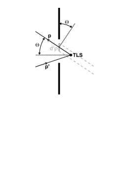
Figure 8: The orifice with the path of the electron scattered by the TLS on the right. The current flows through the surface element $d^{2}\varrho$ and the angle $\theta$ is also indicated.

IV.1.1 Current correction related to inelastic scattering

Using the expression of the collisison term $I_{{\mathbf{R}},\rm TLS,in}$ (71) the change in the current due to the inelastic scattering can be written as

$$\delta I_{{\mathbf{R}},{\rm in}}=\frac{2e}{\hbar}{\rm sign}(R_{z})\int\limits_{\mathbf{p}\in\Omega_{\mathbf{R}}}{{\rm d}\Omega_{\mathbf{p}}\over{4\pi}}\int{\rm d}\varepsilon\;\cos^{2}\theta\int{{\rm d}\Omega_{\mathbf{p}^{\prime}}\over{4\pi}}w_{\hat{\mathbf{p}}\hat{\mathbf{p}}^{\prime}}\int{\rm d}\varepsilon^{\prime}$$

$$\Big{\{}\left[f_{\mathbf{p}^{\prime}}^{0}(1-f_{\mathbf{p}}^{0})n_{-}-f_{\mathbf{p}}^{0}(1-f_{\mathbf{p}^{\prime}}^{0})n_{+}\right]\delta(\varepsilon+E-\varepsilon^{\prime})+\left[f_{\mathbf{p}^{\prime}}^{0}(1-f_{\mathbf{p}}^{0})n_{+}-f_{\mathbf{p}}^{0}(1-f_{\mathbf{p}^{\prime}}^{0})n_{-}\right]\delta(\varepsilon-E-\varepsilon^{\prime})\Big{\}},$$ (90)

where the distribution functions $f^{0}$ are given by Eq. (76) and taken at $\mathbf{r}=\mathbf{R}$, and the dimensionless notation

$$w_{\hat{\mathbf{p}}\hat{\mathbf{p}}^{\prime}}=\hbar\varrho_{0}^{2}W_{\hat{\mathbf{p}}\hat{\mathbf{p}}^{\prime}}$$ (91)

is introduced. The potential $\Phi(\mathbf{R})$ appearing in these expressions can be dropped as the energy integral variables can be shifted. The essential contribution is given by ${eV\over 2}\eta(\mathbf{p},\mathbf{R})=\pm{eV\over 2}$, which has a positive sign if the electron at $\mathbf{r}=\mathbf{R}$ arrives from the left contact and a negative sign if it is arriving from the right contact.

The final expression is

$$\delta I_{\mathbf{R},{\rm in}}=\frac{2e}{\hbar}{\rm sign}(R_{z})\int\limits_{\mathbf{p}\in\Omega_{\mathbf{R}}}{{\rm d}\Omega_{\mathbf{p}}\over{4\pi}}w_{\hat{\mathbf{p}}\hat{\mathbf{p}}^{\prime}}\int{\rm d}\varepsilon\;\cos^{2}\theta\int{{\rm d}\Omega_{\mathbf{p}^{\prime}}\over{4\pi}}\int{\rm d}\varepsilon^{\prime}$$

$$\Bigg{\{}\Big{[}f_{0}(\varepsilon^{\prime}+{eV\over 2}\eta(\mathbf{p}^{\prime}))(1-f_{0}(\varepsilon+{eV\over 2}\eta(\mathbf{p})))n_{-}-f_{0}(\varepsilon+{eV\over 2}\eta(\mathbf{p}))(1-f_{0}(\varepsilon^{\prime}+{eV\over 2}\eta(\mathbf{p}^{\prime})))n_{+}\Big{]}\delta(\varepsilon+E-\varepsilon^{\prime})+$$

$$\Big{[}f_{0}(\varepsilon^{\prime}+{eV\over 2}\eta(\mathbf{p}^{\prime}))(1-f_{0}(\varepsilon+{eV\over 2}\eta(\mathbf{p})))n_{+}-f_{0}(\varepsilon+{eV\over 2}\eta(\mathbf{p}))(1-f_{0}(\varepsilon^{\prime}+{eV\over 2}\eta(\mathbf{p}^{\prime})))n_{-}\Big{]}\delta(\varepsilon-E-\varepsilon^{\prime})\Bigg{\}}.$$

This expression can be divided into two parts. If the electron with momentum $\mathbf{p}^{\prime}$ arrives from the same side of the contact ($|\mathbf{r}|\to\infty$) as the unscattered electron with momentum $\mathbf{p}$, thus $\eta(\mathbf{p})\eta(\mathbf{p}^{\prime})=1$, then the electron is scattered forward, while for $\eta(\mathbf{p})\eta(\mathbf{p}^{\prime})=-1$ it is scattered backward (see Fig. 9). The total current can be divided according to that, thus

$$\delta I_{\mathbf{R},{\rm in}}=\delta I_{\mathbf{R},{\rm in,for}}+\delta I_{\mathbf{R},{\rm in,back}}.$$ (93)

Figure 9: The paths for forward (grey line) and backscattering (black line) are shown with the TLS on the right (a) or left (b). The $\eta$ signs are also indicated.

The forward scattering cancels out. That can be seen by looking e.g. the first and the last term in the previous expression and changing $\varepsilon\leftrightarrow\varepsilon^{\prime}$,

$$\delta I_{\mathbf{R},{\rm in,for}}=0.$$ (94)

In the calculation of the backscattering the case ${\rm sign}(R_{z})=1$ is taken first. Then the electron contributing to the current originally comes from the left ($\eta(\mathbf{p}^{\prime})=1$) and after the scattering goes from right to the left ($\eta(\mathbf{p})=-1$).

$$\delta I_{\mathbf{R},{\rm in,back}} = \frac{2e}{\hbar}\int\limits_{\mathbf{p}\in\Omega_{\mathbf{R}}}{{\rm d}\Omega_{\mathbf{p}}\over{4\pi}}\int{\rm d}\varepsilon\;\cos^{2}\theta\int\limits_{{-\mathbf{p}\;^{\prime}\in\Omega_{\mathbf{R}}}}{{\rm d}\Omega_{\mathbf{p}^{\prime}}\over{4\pi}}\int{\rm d}\varepsilon^{\prime}\;w_{\hat{\mathbf{p}}\hat{\mathbf{p}}^{\prime}}\cdot$$ (95)

$$\Bigg{\{}\Big{\{}f_{0}(\varepsilon^{\prime}+{eV\over 2})(1-f_{0}(\varepsilon-{eV\over 2}))n_{-}-f_{0}(\varepsilon-{eV\over 2})(1-f_{0}(\varepsilon^{\prime}+{eV\over 2}))n_{+}\Big{\}}\delta(\varepsilon+E-\varepsilon^{\prime})$$

$${+} \Big{\{}f_{0}(\varepsilon^{\prime}+{eV\over 2})(1-f_{0}(\varepsilon-{eV\over 2}))n_{+}-f_{0}(\varepsilon-{eV\over 2})(1-f_{0}(\varepsilon^{\prime}+{eV\over 2}))n_{-}\Big{\}}\delta(\varepsilon-E-\varepsilon^{\prime})\Bigg{\}}.$$

The factor due to the angular integrals $\int\limits_{\mathbf{p}\in\Omega_{\mathbf{R}}}{{\rm d}\Omega_{\mathbf{p}}\over{4\pi}}\cos^{2}\theta\int\limits_{{-\mathbf{p}\;^{\prime}\in\Omega_{\mathbf{R}}}}{{\rm d}\Omega_{\mathbf{p}^{\prime}}\over{4\pi}}w_{\hat{\mathbf{p}}\hat{\mathbf{p}}^{\prime}}$ plays the role of the geometrical factor for the bulk phonons. Only the backscattering contributes like in the case of phonons as it can be seen from Eq. (67) for ballistic regions where the $K$-factor contains the factor $\Theta(-\hat{p}_{z}\hat{p}_{z}^{\prime})$.

In the following the geometrical factor is introduced which depends on the position of the TLS, $\mathbf{R}$, and it is independent of the strength of the interaction

$$K_{\mathbf{R}}={1\over w}\int\limits_{\mathbf{p}\in\Omega_{\mathbf{R}}}{{\rm d}\Omega_{\mathbf{p}}\over{4\pi}}\cos^{2}\theta\int\limits_{{-\mathbf{p}^{\prime}\in\Omega_{\mathbf{R}}}}{{\rm d}\Omega_{\mathbf{p}^{\prime}}\over{4\pi}}w_{\hat{\mathbf{p}}\hat{\mathbf{p}}^{\prime}},$$ (96)

where

$$w=\int{{\rm d}\Omega_{\mathbf{p}}\over{4\pi}}\int{{\rm d}\Omega_{\mathbf{p}^{\prime}}\over{4\pi}}w_{\hat{\mathbf{p}}\hat{\mathbf{p}}^{\prime}}.$$ (97)

If the momentum dependence of the interaction is ignored then $w_{\hat{\mathbf{p}}\hat{\mathbf{p}}^{\prime}}=w$ and

$$K_{\mathbf{R}}=\int\limits_{\mathbf{p}\in\Omega_{\mathbf{R}}}{{\rm d}\Omega_{\mathbf{p}}\over{4\pi}}\cos^{2}\theta\int\limits_{{-\mathbf{p}^{\prime}\in\Omega_{\mathbf{R}}}}{{\rm d}\Omega_{\mathbf{p}^{\prime}}\over{4\pi}}$$ (98)

is a pure geometrical factor. Further on this simplification is assumed. If the TLS is positioned on the geometrical axis of a circular contact then the above integral can be evaluated as

$$K_{\mathbf{R}}=\left(\frac{\Omega_{\mathbf{R}}}{4\pi}\right)^{2}\left(1-\frac{4}{3}\left(\frac{\Omega_{\mathbf{R}}}{4\pi}\right)^{2}\right).$$ (99)

In the second part of the integral in Eq. (95) the variables are changed as $\varepsilon\leftrightarrow\varepsilon^{\prime}$ and the integral with respect $\varepsilon^{\prime}$ is performed, furthermore, in some of the integrals the variable is shifted as $\varepsilon-{eV\over 2}\to\varepsilon$. The result is

$$\delta I_{{\mathbf{R}},{\rm in,back}}=\frac{2e}{\hbar}wK_{\mathbf{R}}\int{\rm d}\varepsilon\;f_{0}(\varepsilon) \Big{\{} \left[f_{0}(\varepsilon-E+eV)-f_{0}(\varepsilon-E-eV)\right]n_{-}$$ (100)

$$+ \left[f_{0}(\varepsilon+E+eV)-f_{0}(\varepsilon+E-eV)\right]n_{+}\Big{\}}.$$

Now the TLS on the left is considered (sign$(R_{z})=-1$). Then for backscattering the signs of $\eta(\mathbf{p})$ and $\eta(\mathbf{p}^{\prime})$ are reversed (see Fig. 9b) That is equivalent of changing the sign of $V$ ($V\to-V$) in Eq. (95) and then the expression in the curly bracket also changes its sign as it can be seen by inserting $\varepsilon\leftrightarrow\varepsilon^{\prime}$. That negative sign is cancelled by sign$(R_{z})=-1$, thus the total current is unchanged. Therefore, the current does not depend on whether the TLS is on the right or left as it should be.

After inserting the Fermi functions and performing the energy integral, the following result is obtained for the inelastic current correction:

$$\delta I_{\mathbf{R},\rm in}=n_{-}C+n_{+}D,$$ (101)

where

$$C=\frac{2e}{\hbar}wK_{\mathbf{R}}\left\{{eV+E\over{2}}\Bigg{[}\coth({eV+E\over{2k_{B}T}})-1\Bigg{]}-{E-eV\over{2}}\Bigg{[}\coth({E-eV\over{2k_{B}T}})-1\Bigg{]}\right\},$$

$$D=\frac{2e}{\hbar}wK_{\mathbf{R}}\left\{{eV-E\over{2}}\Bigg{[}\coth({eV-E\over{2k_{B}T}})-1\Bigg{]}-{-E-eV\over{2}}\Bigg{[}\coth({-E-eV\over{2k_{B}T}})-1\Bigg{]}\right\}.$$ (102)

These expressions are simplified at $T=0$ as

$$\delta I_{\mathbf{R},\rm in}=-\frac{2e}{\hbar}wK_{\mathbf{R}}{\rm sign}(V)\left\{\begin{array}[]{lr}2e|V|n_{+}&e|V|<E\\ &\\ 2En_{+}+(e|V|-E)&e|V|\geq E\end{array}\right..$$ (103)

If the TLS was in thermal equilibrium with the bath, at zero temperature $n_{+}=0$ and $n_{-}=1$ would hold. In that case the voltage dependence of the conductance is easily evaluated, it contains a jump-like decrease at the excitation energy of the TLS:

$$\delta G_{\mathbf{R},\rm in}={\partial\delta I_{\mathbf{R},\rm{in}}\over{\partial V}}=-\frac{2e^{2}}{\hbar}wK_{\mathbf{R}}\cdot\Theta(e|V|-E),$$ (104)

where $\Theta(x)=\Big{\{}{{1\;{\rm for}\;x>0}\atop{{0\;{\rm for}\;x\leq 0}}}$. That result means if the TLS is in the ground state $n_{-}=1$ then the TLS can be excited only by a voltage $e|V|>E$, where the backscattering reduces the current. The second derivative has a Dirac delta peak at the excitation energy

$${\partial^{2}\delta I_{\mathbf{R},\rm in}\over{\partial V^{2}}}={\partial\delta G_{\mathbf{R},\rm in}\over{\partial V}}=-\frac{2e^{3}}{\hbar}wK_{\mathbf{R}}{\rm sign}(V)\cdot\delta(e|V|-E).$$ (105)

This result is similar to the phonon result, that is the ${\partial^{2}I\over{\partial V^{2}}}$ shows the structure of the excitation spectrum of a scatterer in the contact region. However, for a TLS situated in the contact region the occupation of the upper level is not zero, as the system is driven out of equilibrium. Due to this feature a nontrivial contribution occurs in the background resistance beside the spectroscopic feature at the excitation energy. This can be evaluated after calculating the voltage dependence of the occupation number, $n_{+}(V)$, which is performed later in this section.

IV.1.2 Elastic scattering

A similar calculation can be performed for the current correction due to the elastic scattering on TLSs by using the collision integral $I_{\mathbf{R},\rm TLS,el}(\mathbf{p},\mathbf{r})$ (73) instead of $I_{\mathbf{R},\rm TLS,in}(\mathbf{p},\mathbf{r})$ (71). The formulas for the elastic scattering can be derived easily by inserting $E=0$ and modifying the scattering strength in the results for the inelastic case. For elastic scattering the strength of the interaction can be different for the TLS being in the “$+$” and “$-$” state, thus in Eq. (IV.1.1) $wK_{\mathbf{R}}$ must be replaced by $[wK_{\mathbf{R}}]^{-}$ and $[wK_{\mathbf{R}}]^{+}$ in the expression for $C$ and $D$, respectively. After these considerations the result is:

$$\delta I_{\mathbf{R},\rm el}=-\frac{2e^{2}V}{\hbar}\left(n_{-}\cdot[wK_{\mathbf{R}}]^{-}+n_{+}\cdot[wK_{\mathbf{R}}]^{+}\right).$$ (106)

Note, that in the elastic case the voltage dependent “$\coth(\cdots)$” terms cancel out, thus the only voltage dependence comes from the voltage dependence of the occupation number. If the TLS is in thermal equilibrium with the bath, then $n_{+}=1-n_{-}=0$ holds, thus the elastic current correction is a voltage independent constant term. Similarly, if the scattering cross sections for the two states of the TLS are equal, then the voltage dependence cancels out due to the condition $n_{+}+n_{-}=1$. In the following we use a simplified notation for the elastic current correction:

$$\delta I_{\rm el}=-V(\gamma^{-}n_{-}+\gamma^{+}n_{+}),$$ (107)

where $\gamma^{+}$ and $\gamma^{-}$ are considered as the reduction of the conductance due to the TLS being in the “$+$” and the “$-$” state, respectively.Kozub (1986) The average change in the conductance due to the elastic scattering is characterized by $\frac{\gamma^{+}+\gamma^{-}}{2}$, which is written as follows according to formulas (106, 98, 91, IV.1):

$$\frac{\gamma^{+}+\gamma^{-}}{2}=\frac{2e^{2}}{h}(2\pi)^{2}K_{\mathbf{R}}\varrho_{0}^{2}\left(\left[V^{0}\right]^{2}+\left[(\mu^{2}-\nu^{2})V^{z}\right]^{2}\right),$$ (108)

where $V^{0}$ and $V^{z}$ are the the interaction matrix elements from Eq. (11) assuming isotropic scattering. The difference between the conductances corresponding to the two states of the TLS are written as:

$$\gamma^{+}-\gamma^{-}=\frac{2e^{2}}{h}(2\pi)^{2}K_{\mathbf{R}}\varrho_{0}^{2}(4\mu^{2}-4\nu^{2})V^{0}V^{z}.$$ (109)

Again, the voltage dependence of the current correction can only be determined after calculating the occupation number as a function of bias voltage, which is done in the following part. It is important to note that in case $V^{0}=0$ the scattering strength is symmetric for the two states, thus $\gamma^{+}=\gamma^{-}$.

IV.1.3 Calculation of the occupation number

In the following $n_{+}$ will be calculated in the nonequilibrium case, where it is determined by the interaction with the nonequilibrium electrons. The transition probability from the “$-$” to the “$+$” state due to an electron scattered from momentum state $\mathbf{p}$ to $\mathbf{p}^{\prime}$ has been considered in the collision term (71) and it is:

$$W_{\mathbf{R}}^{+-}(\mathbf{p}^{\prime}\mathbf{p})=W_{\hat{\mathbf{p}}^{\prime}\hat{\mathbf{p}}}n_{-}f_{\mathbf{p}}(\mathbf{R})(1-f_{\mathbf{p}^{\prime}}(\mathbf{R}))\delta(\varepsilon_{\mathbf{p}}-\varepsilon_{\mathbf{p}^{\prime}}-E),$$ (110)

and similarly:

$$W_{\mathbf{R}}^{-+}(\mathbf{p}^{\prime}\mathbf{p})=W_{\hat{\mathbf{p}}^{\prime}\hat{\mathbf{p}}}n_{+}f_{\mathbf{p}}(\mathbf{R})(1-f_{\mathbf{p}^{\prime}}(\mathbf{R}))\delta(\varepsilon_{\mathbf{p}}-\varepsilon_{\mathbf{p}^{\prime}}+E).$$ (111)

The transition probabilities for the TLS are obtained after integrating for the electron momenta:

$$W_{\mathbf{R}}^{+-\atop{-+}}=n_{\mp}{1\over\hbar}\int{{\rm d}\Omega_{\mathbf{p}}\over{4\pi}}\int{{\rm d}\Omega_{\mathbf{p}^{\prime}}\over{4\pi}}w_{\hat{\mathbf{p}}^{\prime}\hat{\mathbf{p}}}\int{\rm d}\varepsilon\Big{\{}f_{0}(\varepsilon-e\Phi(\mathbf{R})+{eV\over 2}\eta(\mathbf{p}))(1-f_{0}(\varepsilon\mp E-e\Phi(\mathbf{R})+{eV\over 2}\eta(\mathbf{p}^{\prime}))\Big{\}},$$

where the expression (76) for $f_{\mathbf{p}}(\mathbf{R})$ is used.

The kinetic equation for $n_{+}$ is:

$${{\rm d}n_{+}\over{{\rm d}t}}=W_{\mathbf{R}}^{+-}-W_{\mathbf{R}}^{-+}.$$ (113)

In the Fermi functions the electron momentum is only involved in $\eta(\mathbf{p})$, which tells which reservoir the electron at position $\mathbf{R}$ with momentum $\mathbf{p}$ is coming from. Therefore the integral can be performed by separating the regions of integration into four cases with respect to the possible values of $\eta(\mathbf{p})$ and $\eta(\mathbf{p}^{\prime})$. In all of these four regions the factor containing the Fermi functions is independent of $\Omega_{\mathbf{p}}$ and $\Omega_{\mathbf{p}}^{\prime}$. There is an essential simplification if $w_{\hat{\mathbf{p}}\hat{\mathbf{p}}^{\prime}}$ is replaced by a momentum independent averaged one, $w$. Take e.g. the case where the TLS is on the right hand side of the contact ($R^{z}>0$) and introduce the solid angle $\Omega_{\mathbf{R}}$ at which the opening can be seen from point $\mathbf{R}$. In this case the integrals for the different regions are written as:

$$W_{\mathbf{R}}^{+-\atop{-+}}=n_{\mp}\frac{w}{\hbar}\int(\cdots){\rm d}\varepsilon\cdot\left\{\begin{array}[]{ll}({\Omega_{\mathbf{R}}\over 4\pi})^{2}&\quad{\rm if}\quad\eta(\mathbf{p})=1,\;\;\eta(\mathbf{p}^{\prime})=1\\ &\\ (1-{\Omega_{\mathbf{R}}\over 4\pi})^{2}&\quad{\rm if}\quad\eta(\mathbf{p})=-1,\;\;\eta(\mathbf{p}^{\prime})=-1\\ &\\ {\Omega_{\mathbf{R}}\over 4\pi}(1-{\Omega_{\mathbf{R}}\over 4\pi})&\quad{\rm if}\quad\eta(\mathbf{p})=1,\;\;\eta(\mathbf{p}^{\prime})=-1\\ &\\ {\Omega_{\mathbf{R}}\over 4\pi}(1-{\Omega_{\mathbf{R}}\over 4\pi})&\quad{\rm if}\quad\eta(\mathbf{p})=-1,\;\;\eta(\mathbf{p}^{\prime})=1\end{array}\right.,$$ (114)

This simplification is justified only after taking an average over large number of TLSs but that simplifies the calculation and makes the result more transparent. In this simplified case the kinetic equation for the TLS is obtained after calculating the energy integrals for the different cases. (As before, $e\Phi(\mathbf{R})$ is eliminated by shifting the integral variables.) The final result is independent whether the TLS is on the right or left, and it can be written in the form:

$${{dn_{+}}\over{dt}}=n_{-}A-n_{+}B=A-n_{+}(A+B),$$ (115)

where the coefficients $A$ and $B$ are:

$$A={w\over\hbar}\Bigg{\{}\left(1-\frac{\Omega_{\mathbf{R}}}{4\pi}\right)\frac{\Omega_{\mathbf{R}}}{4\pi}\left[\frac{eV+E}{2}\left(\coth(\frac{eV+E}{2k_{B}T})-1\right)+\frac{-eV+E}{2}\left(\coth(\frac{-eV+E}{2k_{B}T})-1\right)\right]+$$

$$+\left(\left(1-\frac{\Omega_{\mathbf{R}}}{4\pi}\right)^{2}+\left(\frac{\Omega_{\mathbf{R}}}{4\pi}\right)^{2}\right)\frac{E}{2}\left[\coth(\frac{E}{2k_{B}T})-1\right]\Bigg{\}},$$

$$B={w\over\hbar}\Bigg{\{}\left({1-{\Omega_{\mathbf{R}}\over{4\pi}}}\right){\Omega_{\mathbf{R}}\over{4\pi}}\left[{{eV-E\over{2}}\left({\coth({eV-E\over{2k_{B}T}})-1}\right)+{-eV-E\over{2}}\left({\coth({-eV-E\over{2k_{B}T}})-1}\right)}\right]+$$

$$+\left({\left({1-{\Omega_{\mathbf{R}}\over{4\pi}}}\right)^{2}+\left({{\Omega_{\mathbf{R}}\over{4\pi}}}\right)^{2}}\right){-E\over 2}\left[{\coth({-E\over{2k_{B}T}})-1}\right]\Bigg{\}},$$ (116)

respectively. The relaxations are of Korringa types, which depend on $V$ only if the two electrons involved have different chareacters in terms of $\eta(\mathbf{p})$. The stationary value of $n_{+}$ is obtained as

$$n_{+}={A\over{A+B}},$$ (117)

which is an even function of $V$. At $T=0$ this expression simplifies essentially:

$$n_{+}=\Bigg{\{}\begin{array}[]{lr}0&e|V|<E\\ \frac{1}{2}-\frac{E}{2E+4\kappa(e|V|-E)}&e|V|\geq E\end{array},$$ (118)

where $\kappa={\Omega_{\mathbf{R}}\over 4\pi}(1-{\Omega_{\mathbf{R}}\over 4\pi})$. $n_{+}$ is a continuous function of $V$. Far from the opening $\kappa\to 0$ thus $n_{+}\to 0$ at voltages for which $(e|V|-E)/E\ll\kappa^{-1}$ as the electron gas is in thermal equilibrium. For $\kappa={\rm const.}$ and $(e|V|-E)/E\gg\kappa^{-1}$ $n_{+}\to{1\over 2}$ as for large enough voltage the levels are equally occupied $n_{-}=n_{+}={1\over 2}$. If the TLS is in the middle of the contact, then $\kappa=1/4$.

If the TLS is far away from the contact then it is in thermal equilibrium, which can be obtained by taking $\Omega_{\mathbf{R}}\to 0$ and the deviation from equilibrium is large when the TLS is in the middle of the contact region $\Omega_{\mathbf{R}}=2\pi$. Here other relaxation mechanism different from the scattering of electrons is not taken into account as the generation of bulk phonons is very weak as the relevant phase space is very small at low energies. At large concentration of TLSs the TLSs are interacting and the collective effects may modify the stationary values of the occupation numbers.

IV.1.4 Conductance with inelastic and elastic scattering

Now the inelastic and elastic contributions to the current and the conductance are calculated using the stationary occupation numbers obtained. The expressions will be given when the TLS is just in the middle of the round opening, thus $\Omega_{\mathbf{R}}=2\pi$ ($\kappa={1\over 4}$), but the calculation for arbitrary $\Omega_{\mathbf{R}}$ can be easily performed as well.

At zero temperature the inelastic current correction is obtained by inserting the stationary value of $n_{+}$ given by Eq. (118) into (103):

$$\delta I_{\mathbf{R}=0,\rm in}=-\frac{2e}{\hbar}wK_{\mathbf{R}=0}{\rm sign}(V)\left\{\begin{array}[]{lr}0&e|V|<E\\ e|V|-{2E^{2}\over{E+e|V|}}&e|V|\geq E\end{array}\right.,$$ (119)

which is a continuous function of $V$. After differentiation with respect to the voltage the correction to the conductance is obtained as:

$$\delta G_{\mathbf{R}=0,\rm in} = {\partial\delta I_{\mathbf{R}=0,\rm in}\over{\partial V}}=-\frac{2e^{2}}{\hbar}wK_{\mathbf{R}=0}\left\{\begin{array}[]{lr}0&e|V|<E\\ 1+2{E^{2}\over{(E+e|V|)^{2}}}&e|V|\geq E\end{array}\right.,$$ (122)

and the second derivative of the current is:

$${\partial\delta G_{\mathbf{R}=0,\rm in}\over{\partial V}}=-\frac{2e^{3}}{\hbar}wK_{\mathbf{R}=0}{\rm sign}(V)\left\{{3\over 2}\delta(E-e|V|)-\Theta(e|V|-E){4E^{2}\over{(E+e|V|)^{3}}}\right\}.$$ (123)

At positive voltages the second derivative of the current shows a negative Dirac delta peak at $eV=E$, which reflects the energy spectrum of a single TLS. Above the excitation energy a positive background is seen due to the nonequilibrium distribution of the TLS occupation number.

As a next step the elastic contribution is determined at $T=0$ for a single TLS positioned in the middle of the contact. The change in the conductance due to the elastic scattering can be calculated by differentiating Eq. (107). The elastic current correction contains a linear term, which causes a constant, voltage independent reduction of the conductance. Experimentally it is hard to separate this constant contribution, thus we calculate only the voltage dependent part by subtracting the zero bias conductance:

$$\delta G_{\mathbf{R}=0,\rm el}=\frac{\partial\delta I_{\mathbf{R}=0,\rm el}}{\partial V}-\left.\frac{\partial\delta I_{\mathbf{R}=0,\rm el}}{\partial V}\right|_{V=0}=-(\gamma^{+}-\gamma^{-})\left\{\begin{array}[]{lr}0&e|V|<E\\ \frac{1}{2}-\frac{E^{2}}{(E+e|V|)^{2}}&e|V|\geq E\end{array}\right.,$$ (124)

The second derivative of the $I(V)$ curve is

$${\partial\delta G_{\mathbf{R}=0,\rm el}\over{\partial V}}=-e(\gamma^{+}-\gamma^{-}){\rm sign}(V)\left\{\frac{1}{4}\delta(E-e|V|)+\Theta(e|V|-E)\frac{2E^{2}}{(E+e|V|)^{3}}\right\}.$$ (125)

Again, a Dirac delta peak reflects the spectrum of the TLS, and a continuous background arises at $e|V|>E$ due to the nonequilibrium distribution. Contrary to the inelastic case, the Dirac delta peak and the background have the same sign; furthermore, in the elastic case the sign of the peak can either be positive or negative depending on the sign of $\gamma^{+}-\gamma^{-}$. The amplitude $\gamma^{+}-\gamma^{-}$ is related to the universal conductance fluctuation $2e^{2}/h$ (see e.g. Lee, 1986).

For arbitrary position of the TLS the occupation number $n_{+}$ is zero at $V=0$ and $1/2$ at $V\to\infty$. Therefore, the total amplitudes for the change in the conductance in the elastic and inelastic case can be generally written as:

$$\Delta G_{\mathbf{R},\rm in}=-\frac{2e^{2}}{\hbar}wK_{\mathbf{R}} = \frac{2e^{2}}{h}(2\pi)^{2}K_{\mathbf{R}}\varrho_{0}^{2}(2\mu\nu)^{2}(V^{z})^{2}$$ (126)

$$\Delta G_{\mathbf{R},\rm el}=-\frac{1}{2}(\gamma^{+}-\gamma^{-}) = \frac{2e^{2}}{h}(2\pi)^{2}K_{\mathbf{R}}\varrho_{0}^{2}(2\mu^{2}-2\nu^{2})V^{0}V^{z},$$ (127)

where isotropic scattering was assumed, and the formulas (70, 91, 98, 109) were used. The results are given in the unit of the universal conductance quantum, $2e^{2}/h$. According to Eq. (7) for a highly asymmetric TLS, where the energy splitting $\Delta$ is much larger than the transition term $\Delta_{0}$, the equations $\mu\simeq 1$ and $\nu\simeq 0$ hold. In this case the inelastic term is suppressed. In the opposite case, where $\Delta\ll\Delta_{0}$ the elastic term is suppressed as $\mu\simeq\nu\simeq 1/2$. It must be also noted that the inelastic term depends only on the matrix element $V^{z}$, whereas the elastic term is influenced both by $V^{z}$ and $V^{0}$. The inelastic term can be roughly estimated as $\Delta G_{\mathbf{R},\rm in}\lesssim 0.02\,\frac{2e^{2}}{h}$ using $K_{\mathbf{R}=0}=1/6$, $\mu=\nu=1/2$, $\varrho_{0}V^{z}\sim 0.1$ (see Vladar1983a, ; Vladar1983c, ). The amplitude sharply drops by moving the TLS further from the orifice than its diameter because of the geometrical factor. The estimation of the elastic term is more difficult as $V^{0}$ is strongly model dependent.

In the following the effect of a TLS is considered at finite temperature. The formulas for the conductance and the second derivative of the $I(V)$ curve can be explicitly calculated using equations (101, IV.1.1, 106, IV.1.3, 117); however, these equations are very complicated, thus the results are demonstrated by figures. Figure 10 shows the voltage dependence of the conductance for the inelastic and elastic case respectively. In Fig. 11 the second derivative of the $I(V)$ curve, the so-called point contact spectrum is presented at various temperatures both for the elastic and inelastic case. In Fig. 12 both the inelastic and elastic contributions are compared for a TLS positioned in the contact center ($\Omega_{\mathbf{R}}=2\pi$) and for a TLS being farther away ($\Omega_{\mathbf{R}}=2\pi/5$).

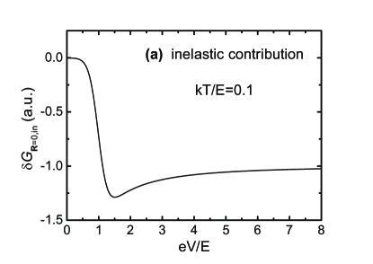
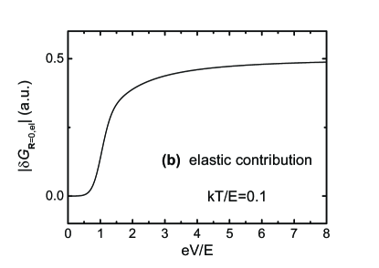
Figure 10: The contribution of the elastic and inelastic scattering to the resistivity in the ballistic limit when the TLS is in the center of the contact ($\delta G_{\mathbf{R}=0,\rm in}$ and $\delta G_{\mathbf{R}=0,\rm el}$, respectively). The temperature is $kT=0.1E$. The sign of the elastic contribution can be either positive or negative depending on the sign of ($\gamma^{+}-\gamma^{-}$). On the other hand, the inelastic scattering always causes a decrease in the conductance.

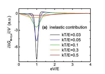
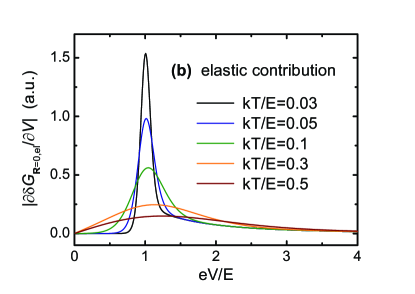
Figure 11: The second derivative of the $I(V)$ curve for inelastic and elastic scattering at various temperatures for a ballistic point contact ($\partial\delta G_{\mathbf{R}=0,\rm in}/\partial V$, and $\partial\delta G_{\mathbf{R}=0,\rm el}/\partial V$, respectively). The inelastic contribution shows a negative peak at the excitation energy of the TLS and a positive background tail at higher voltages. The elastic contributions similarly shows a peak at $eV=E$ and a background tail at higher voltages, but here the sign of the peak and the tail is the same. In the elastic case the sign of the signal can either be positive or negative depending on the sign of ($\gamma^{+}-\gamma^{-}$).

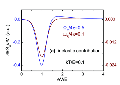
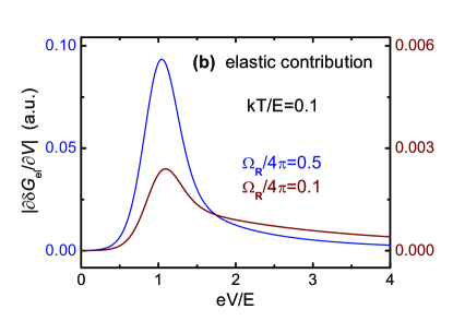
Figure 12: The second derivative of the $I(V)$ curve for inelastic and elastic scattering for two different positions of the TLS: in one case the TLS is in the contact center, in the other case it is farther away on the contact axis, so that the opening is seen in a solid angle $\Omega_{\mathbf{R}}=4\pi/10$. The TLS being farther away from the contact is closer to thermal equilibrium, which is reflected by the reduced amplitude of the background tail with respect to the spectroscopic peak in the inelastic contribution.

IV.2 Slow TLS in a diffusive contact

As it has been discussed in Sec. III.1 the phenomenological treatment must be replaced by a theory based on kinetic equation, where effect of the inelastic scatterings are taken into account in the distribution function. In the following the elastic and inelastic scatterings are treated in equal footing. As a first step the distribution function is determined in the presence of elastic scattering and next the contributions of the TLS are treated as a perturbation.

Consider first the elastic scattering in the limit $l_{\rm el}\to 0$, where the resistance is very large. Because of the very strong elastic scattering, the electrons are immediately redistributed concerning the direction of their momenta. Therefore, in the limit $l_{\rm el}\to 0$ the distribution function depends only on the energy of the electrons, $f_{\mathbf{p}}(\mathbf{r})\to f_{\varepsilon}(\mathbf{r})$. As the electron arriving at the contact is either coming from the left or the right reservoirs and the electron energies are changed due to the external potential $\Phi(\mathbf{r})$ the distribution function must be the superposition of the distribution of the electrons coming from the left or right with amplitudes $\alpha_{0}(\mathbf{r})$ and $1-\alpha_{0}(\mathbf{r})$, respectively:

$$f_{\varepsilon}(\mathbf{r})=\alpha_{0}(\mathbf{r})f_{0}(\varepsilon_{\mathbf{p}}-e\Phi(\mathbf{r})+{eV\over 2})+\Big{(}1-\alpha_{0}(\mathbf{r})\Big{)}f_{0}(\varepsilon_{\mathbf{p}}-e\Phi(\mathbf{r})-{eV\over 2}).$$ (128)

Using the charge neutrality condition ($\int f_{\epsilon}(\mathbf{r}){\rm d}\varepsilon=\int f_{0}(\epsilon_{\mathbf{p}}){\rm d}\varepsilon)$ $\alpha_{0}(\mathbf{r})$ can be determined by a similar treatment used earlier in case of Eq. (58):

$$\alpha_{0}(\mathbf{r})={1\over 2}+{\Phi(\mathbf{r})\over V}.$$ (129)

This formula is valid in case of arbitrary geometry because only the shape of the potential function contains information about the details of the geometry. For an opening type circular contact the potential was determined in Sec. III.1 by solving the Laplace equation using a hyperbolic coordinate system.

Figure 13: Visualization of the distribution function in the diffusive limit. Without inelastic processes the smearing of the two steps are due to the finite temperature, $T$.

The distribution function contains two sharp steps due to the two different Fermi energies in the two reservoirs (see Fig. 13). Such steps are measured by the Saclay group studying short metallic wires of type Fig. LABEL:PCmodels.figb by attaching an extra tunneling diode on the side of the wire. (See Pothier, 1997; Gougam, 2000).

In the ballistic limit the distribution function is very similar only the factors $\alpha_{0}(\mathbf{r})$ and $1-\alpha_{0}(\mathbf{r})$ are replaced by the geometrical factors $\frac{\Omega(\mathbf{r})}{4\pi}$ and $1-\frac{\Omega(\mathbf{r})}{4\pi}$ determining the solid angles in which the ballistic electron arrives from the left or right reservoirs to the point $\mathbf{r}$.

The electron distribution function (128) obtained for $l_{\rm el}\to 0$ does not result in any current in agreement that the resistivity is infinite in this limit. For finite $l_{\rm el}\ll d$ the factor $\alpha_{0}(\mathbf{r})$ must be replaced by a momentum dependent one $\alpha_{\mathbf{p}}(\mathbf{r})$, and the current is due to $\delta\alpha_{\mathbf{p}}(\mathbf{r})=\alpha_{\mathbf{p}}(\mathbf{r})-\alpha_{0}(\mathbf{r})$, which has a strong asymmetric momentum dependence and $\delta\alpha_{\mathbf{p}}(\mathbf{r})\to 0$ as $l_{\rm el}\to 0$.

The $\delta\alpha_{\mathbf{p}}(\mathbf{r})$ will be determined by the very elegant theory of Kulik, Shekter and Shkorbatov,Kulik (1981) who have extended the treatment of the ballistic limit to the diffusive one treating the scattering on phonons and defects which are large in space. The strong elastic scattering on defects is combined with a weak inelastic scattering. The limit considered is specified as $(l_{\rm el}l_{\rm in})^{1/2}\gg d$ where $d$ is the size of the contact and $l_{\rm el}$ and $l_{\rm in}$ are the elastic and inelastic mean free paths of the electrons, respectively. Introducing the corresponding relaxation times, $\tau_{\rm el}$ and $\tau_{\rm in}$ the inequality can be rewritten as $(\tau_{\rm el}\tau_{\rm in})^{1/2}\gg{d\over v_{F}}$. That means that an electron can diffuse out from the contact region of size $d$ with small probability of inelastic scattering, thus double inelastic scatterings can be neglected. In the following $\tau_{\rm in}$ is related to the relaxation time due to TLSs.

Also in the diffusive limit the current correction due to the TLSs is derived by solving the Boltzman equation (65) with an appropriate collision term. In this case the collision integral $I(\mathbf{p},\mathbf{r})$ has two contributions as the elastic impurity part $I_{\rm el}(\mathbf{p},\mathbf{r})$ and the contribution of individual TLSs at position $\mathbf{R}$, $I_{\rm TLS,\mathbf{R}}(\mathbf{p},\mathbf{r})$ thus

$$I(\mathbf{p},\mathbf{r})=I_{\rm el}(\mathbf{p},\mathbf{r})+\sum\limits_{n}I_{\rm TLS,\mathbf{R}_{n}}(\mathbf{p},\mathbf{r}),$$ (130)

where the sum is due to different TLSs, but in the following it is assumed that the concentration of the TLSs is so low that first a single TLS at position $\mathbf{R}$ is considered and in the final result the contributions of the different TLSs are additive.

The kinetic equation can be arranged as

$$\mathbf{v}_{\mathbf{p}}{\partial f_{\mathbf{p}}(\mathbf{r})\over{\partial\mathbf{r}}}-e\mathbf{E}{\partial f_{\mathbf{p}}(\mathbf{r})\over{\partial\mathbf{p}}}-I_{\rm el}(\mathbf{p},\mathbf{r})=I_{\rm TLS,\mathbf{R}}(\mathbf{p},\mathbf{r}).$$ (131)

First the left hand side is treated in the diffusive limit and the right hand side is considered as a weak perturbation.

The impurity part of the collision integral is

$$I_{\rm el}(\mathbf{p},\mathbf{r})=\frac{1}{(2\pi\hbar)^{3}}\int\limits_{\varepsilon_{\mathbf{p}}=\varepsilon_{\mathbf{p}^{\prime}}}{{\rm d}S_{\mathbf{p}^{\prime}}\over{v_{\perp}^{\prime}}}W_{\mathbf{p}\mathbf{p}^{\prime}}^{\rm imp}\left(f_{\mathbf{p}^{\prime}}(\mathbf{r})-f_{\mathbf{p}}(\mathbf{r})\right),$$ (132)

where $W_{\mathbf{p}\mathbf{p}^{\prime}}^{\rm imp}$ is the elastic transition probability, $v_{\perp}^{\prime}$ is the velocity at momentum $\mathbf{p}^{\prime}$ perpendicular to the equienergetic surface for which the integral is performed. The electric field can be expressed by the electric potential $\Phi(\mathbf{r})$ as $\mathbf{E}=-\nabla_{\mathbf{r}}\Phi(\mathbf{r})$, where $\Phi$ is determined by the neutrality condition as in the ballistic case.

The distribution function $f_{\mathbf{p}}(\mathbf{r})$ satisfies the following boundary condition: At the boundary, $\Sigma$ between the insulator and the metal we assume mirror reflection

$$f_{\mathbf{p}}(\mathbf{r}\in\Sigma)=f_{\tilde{\mathbf{p}}}(\mathbf{r}\in\Sigma),$$ (133)

where an incoming electron with momentum $\mathbf{p}$ is reflected with the momentum $\tilde{\mathbf{p}}$. Furthermore, very far from the contact $|\mathbf{r}|\to\infty$ the equilibrium distribution is recovered with chemical potential $\mu$, thus

$$f_{\mathbf{p}}(|\mathbf{r}|\to\infty)=f_{0}(\varepsilon_{\mathbf{p}})={1\over{e^{{\varepsilon_{\mathbf{p}}-\mu}\over{k_{B}T}}+1}},$$ (134)

and $\mu$ satisfies the charge neutrality.

The distribution function in the absence of the collision term due to TLS is denoted by $f_{\mathbf{p}}^{(0)}(\mathbf{r})$ and the first order correction due to the TLS is $f_{\mathbf{p}}^{(1)}(\mathbf{r})$, thus

$$f_{\mathbf{p}}(\mathbf{r})=f_{\mathbf{p}}^{(0)}(\mathbf{r})+f_{\mathbf{p}}^{(1)}(\mathbf{r})+\cdots,$$ (135)

where the higher order corrections are neglected.

The kinetic equation for $f_{\mathbf{p}}^{(0)}(\mathbf{r})$ contains the static impurity contributions, thus

$$\mathbf{v}_{\mathbf{p}}{\partial f_{\mathbf{p}}^{(0)}(\mathbf{r})\over{\partial\mathbf{r}}}-e\mathbf{E}^{(0)}{\partial f_{\mathbf{p}}^{(0)}(\mathbf{r})\over{\partial\mathbf{p}}}-I_{\rm el}(f_{\mathbf{p}}^{(0)}(\mathbf{r}))=0,$$ (136)

and $f_{\mathbf{p}}^{(1)}(\mathbf{r})$ satisfies the equation

$$\mathbf{v}_{\mathbf{p}}{\partial f_{\mathbf{p}}^{(1)}(\mathbf{r})\over{\partial\mathbf{r}}}-e\mathbf{E}^{(0)}{\partial f_{\mathbf{p}}^{(1)}(\mathbf{r})\over{\partial\mathbf{p}}}-I_{\rm el}(f_{\mathbf{p}}^{(1)}(\mathbf{r}))=I_{\rm TLS,\mathbf{R}}(f_{\mathbf{p}}^{(0)}(\mathbf{r}))+e\mathbf{E}^{(1)}{\partial f_{\mathbf{p}}^{(0)}(\mathbf{r})\over{\partial\mathbf{p}}},$$ (137)

where the electric field is also expanded as $\mathbf{E}=\mathbf{E}^{(0)}+\mathbf{E}^{(1)}+\cdots$. The term $I_{\rm TLS,\mathbf{R}}$ is linearized in the collision, thus $f_{\mathbf{p}}(\mathbf{r})$ is replaced by $f_{\mathbf{p}}^{(0)}(\mathbf{r})$.

Similarly, the current is $I=I^{(0)}+I^{(1)}+\cdots$, where

$$I^{(i)}=-2e\int{\rm d}\mathbf{S}\int{{\rm d}^{3}\mathbf{p}\over{(2\pi\hbar)^{3}}}f_{\mathbf{p}}^{(i)}(\mathbf{r})\mathbf{v}_{\mathbf{p}}\qquad\qquad(i=0,1,\cdots),$$ (138)

and the integral with respect ${\rm d}\mathbf{S}$ is taken on a dividing surface representing the point contact.

According to the introductory remarks of this section, at finite elastic mean free path the distribution function can be expressed with a momentum dependent parameter, $\alpha_{\mathbf{p}}(\mathbf{r})$:

$$f_{\mathbf{p}}^{(0)}(\mathbf{r})=\alpha_{\mathbf{p}}(\mathbf{r})f_{0}^{+}+(1-\alpha_{\mathbf{p}}(\mathbf{r}))f_{0}^{-},$$ (139)

where the electrons arriving from far left (right) at the contact have distribution function $f_{0}^{+}$ ($f_{0}^{-}$), thus

$$f_{0}^{\pm}=f_{0}(\varepsilon_{\mathbf{p}}-e\Phi(\mathbf{r})\pm{eV\over 2}).$$ (140)

As the collision term (132) is linear in the distribution function the equation for $f_{\mathbf{p}}^{(0)}(\mathbf{r})$ is satisfied with $\alpha_{\mathbf{p}}(\mathbf{r})$ as well:

$$\mathbf{v}_{\mathbf{p}}{\partial\alpha_{\mathbf{p}}\over{\partial\mathbf{r}}}-e\mathbf{E}^{(0)}{\partial\alpha_{\mathbf{p}}\over{\partial\mathbf{p}}}-I_{\rm el}(\alpha_{\mathbf{p}})=0.$$ (141)

In the $l_{\rm el}\to 0$ limit the solution of this equation is $\alpha_{0}(\mathbf{r})$, given by (129). At finite elastic mean free path $\alpha_{\mathbf{p}}(\mathbf{r})$ can be expanded as:

$$\alpha_{\mathbf{p}}(\mathbf{r})=\alpha_{0}(\mathbf{r})+\delta\alpha_{\mathbf{p}}(\mathbf{r}),$$ (142)

where $\delta\alpha_{\mathbf{p}}(\mathbf{r})$ is the first order term in the small parameter, $\frac{l_{\rm el}}{d}$. The momentum dependent correction, $\delta\alpha_{\mathbf{p}}$ can be determined by a simple argumentation. At non-zero relaxation time the probability $\alpha_{\mathbf{p}}$ can be considered as the momentum independent probability $\alpha_{0}$ taken at the position of the last elastic collision, that is:

$$\alpha_{\mathbf{p}}(\mathbf{r})=\alpha_{0}(\mathbf{r}-\tau_{\rm el}\mathbf{v}_{\mathbf{p}}).$$ (143)

The expansion of this formula in $\tau_{\rm el}$ gives:

$$\delta\alpha_{\mathbf{p}}=-\tau_{\rm el}\mathbf{v}_{\mathbf{p}}{\partial\alpha_{0}\over{\partial\mathbf{r}}}.$$ (144)

The value of $\alpha_{0}$ is determined by the potential, which drops in the contact region, thus $\frac{\partial\alpha_{0}}{\partial\mathbf{r}}\sim\frac{1}{d}$, and $\delta\alpha_{\mathbf{p}}\sim\frac{l_{\rm el}}{d}$.

The value of $\delta\alpha_{\mathbf{p}}$ can also be obtained by inserting (142) into the Boltzmann equation for $\alpha_{\mathbf{p}}$ (141). After neglecting the higher order terms in the small parameters $\frac{l_{\rm el}}{d}$ and $\frac{eV}{\varepsilon_{F}}$ the following simple formula is achieved:

$$\mathbf{v}_{\mathbf{p}}{\partial\alpha_{\mathbf{p}}\over{\partial\mathbf{r}}}-I_{\rm el}(\alpha_{\mathbf{p}})=0.$$ (145)

For isotropic scattering $W^{\rm imp}_{\mathbf{p},\mathbf{p}^{\prime}}=W^{\rm imp}_{\mathbf{p},-\mathbf{p}^{\prime}}$ holds, the relaxation time approximation is appropriate, thus the collision integral is expressed as:

$$I_{\rm el}(\alpha_{\mathbf{p}})=-\frac{\delta\alpha_{\mathbf{p}}}{(2\pi\hbar)^{3}}\int{{\rm d}S_{\mathbf{p}^{\prime}}\over v_{\perp}^{\prime}}W^{\rm imp}_{\mathbf{p}\mathbf{p}^{\prime}}=-{\delta\alpha_{\mathbf{p}}\over{\tau_{\rm el}}},$$ (146)

which provides the relaxation time, $\tau_{\rm el}$ due to the elastic scattering by the impurities. Inserting this result into (145) the formula (144) for $\delta\alpha_{\mathbf{p}}$ is regained.

The next step is to determine $f_{\mathbf{p}}^{(1)}$ using the equation (145) for $\alpha_{\mathbf{p}}$. The boundary condition for $\alpha_{\mathbf{p}}(|\mathbf{r}|\to\infty)=\Theta(-z)$ as very left the electron comes from the left contact where the electrons are in equilibrium thus

$$f_{\mathbf{p}}^{(1)}(|\mathbf{r}|\to\infty)=0.$$ (147)

Furthermore, the collision term contributes to the distribution function only if the system is out of equilibrium, thus $f_{\mathbf{p}}^{(1)}$ is proportional to the electric field. Therefore, the second term $-e\mathbf{E}^{(0)}{\partial f_{\mathbf{p}}^{(1)}\over{\partial\mathbf{p}}}$ in equation (137) can be dropped as it is proportional to $|\mathbf{E}^{(0)}|^{2}$.

The correction to the kinetic equation is determined by Eq. (137) where after linearizing each term in the field the Ansatz with the function $\chi_{\mathbf{p}}(\mathbf{r})$

$$f_{\mathbf{p}}^{(1)}(\mathbf{r})=-e\Phi^{(1)}(\mathbf{r}){\partial f_{\mathbf{p}}^{(0)}\over{\partial\varepsilon}}+\chi_{\mathbf{p}}(\mathbf{r})$$ (148)

can be used. The terms proportional to $\mathbf{E}^{(1)}=-\partial\Phi^{(1)}/\partial\mathbf{r}$ cancel out in Eq. (137). Thus

$$\mathbf{v}_{\mathbf{p}}{\partial\chi_{\mathbf{p}}\over{\partial\mathbf{r}}}-I_{\rm el}(\chi_{\mathbf{p}})=I_{\rm TLS,\mathbf{R}}(f_{\mathbf{p}}^{(0)}(\mathbf{r})),$$ (149)

with the boundary condition $\chi_{\mathbf{p}}(|\mathbf{r}|\to\infty)=0$ and $\chi_{\mathbf{p}}(\mathbf{r}\in\Sigma)=\chi_{\tilde{\mathbf{p}}}(\mathbf{r}\in\Sigma)$. As it will be shown below the change in the distribution due to the collision term containing the interaction with the TLS can be expressed as linear response with the aid of a Green’s function $g_{\mathbf{p}\mathbf{p}^{\prime}}(\mathbf{r},\mathbf{r}^{\prime})$:

$$\chi_{\mathbf{p}}(\mathbf{r})=\int{\rm d}^{3}\mathbf{r}^{\prime}\int{\rm d}^{3}\mathbf{p}^{\prime}g_{\mathbf{p}\mathbf{p}^{\prime}}(\mathbf{r},\mathbf{r}^{\prime})I_{\rm TLS,\mathbf{R}}(f_{\mathbf{p}^{\prime}}^{(0)}(\mathbf{r}^{\prime})),$$ (150)

where

$$\mathbf{v}_{\mathbf{p}}{\partial g_{\mathbf{p}\mathbf{p}^{\prime}}(\mathbf{r},\mathbf{r}^{\prime})\over\partial\mathbf{r}}+I_{\rm el}(g_{\mathbf{p}\mathbf{p}^{\prime}}(\mathbf{r},\mathbf{r}^{\prime}))=-\delta(\mathbf{p}-\mathbf{p}^{\prime})\delta(\mathbf{r}-\mathbf{r}^{\prime}),$$ (151)

and

$$I_{\rm el}(g_{\mathbf{p}\mathbf{p}^{\prime}}(\mathbf{r},\mathbf{r}^{\prime}))=\frac{1}{(2\pi\hbar)^{3}}\int\limits_{\varepsilon_{\mathbf{p}}=\varepsilon_{\mathbf{p}^{\prime\prime}}}{{\rm d}S_{\mathbf{p}^{\prime\prime}}\over{v_{\bot}^{\prime\prime}}}W_{\mathbf{p}\mathbf{p}^{\prime\prime}}^{\rm imp}\left\{g_{\mathbf{p}^{\prime\prime}\mathbf{p}^{\prime}}(\mathbf{r},\mathbf{r}^{\prime})-g_{\mathbf{p}\mathbf{p}^{\prime}}(\mathbf{r},\mathbf{r}^{\prime})\right\},$$ (152)

with the boundary condition $g_{\mathbf{p}\mathbf{p}^{\prime}}(|\mathbf{r}|\to\infty,\mathbf{r}^{\prime})=0$ and $g_{\mathbf{p}\mathbf{p}^{\prime}}(\mathbf{r}\in\Sigma,\mathbf{r}^{\prime})=g_{\tilde{\mathbf{p}}\mathbf{p}^{\prime}}(\mathbf{r}\in\Sigma,\mathbf{r}^{\prime})$. As $g_{\mathbf{p}\mathbf{p}^{\prime}}(\mathbf{r},\mathbf{r}^{\prime})$ is closely related to the correlation function $\langle n_{\mathbf{p}}(\mathbf{r})n_{\mathbf{p}^{\prime}}(\mathbf{r}^{\prime})\rangle$ the time reversal symmetry can be applied as

$$g_{\mathbf{p}\mathbf{p}^{\prime}}(\mathbf{r},\mathbf{r}^{\prime})=g_{-\mathbf{p}^{\prime}-\mathbf{p}}(\mathbf{r}^{\prime},\mathbf{r}).$$ (153)

The function $G_{\mathbf{p}}(\mathbf{r})$ is defined as

$$G_{\mathbf{p}}(\mathbf{r})=\int{\rm d}S^{\prime}{{\rm d}^{3}\mathbf{p}^{\prime}\over{(2\pi\hbar)^{3}}}v_{\mathbf{p}^{\prime}}^{z}g_{\mathbf{p}\mathbf{p}^{\prime}}(\mathbf{r},\mathbf{r}^{\prime}),$$ (154)

where the integral with respect to ${\rm d}S^{\prime}$ is a surface integral of variable $r^{\prime}$ taken on the orifice. This function satisfies the equation

$$\mathbf{v}_{\mathbf{p}}{\partial G_{\mathbf{p}}\over{\partial\mathbf{r}}}+I_{\rm el}\{G_{\mathbf{p}}(\mathbf{r})\}=-v_{\mathbf{p}}^{z}\delta(z),$$ (155)

which follows from the equation (151) defining $g_{\mathbf{p}\mathbf{p}^{\prime}}(\mathbf{r},\mathbf{r}^{\prime})$. The boundary conditions are the usual ones $G_{\mathbf{p}}(|\mathbf{r}|\to\infty)=0$ and $G_{\mathbf{p}}(\mathbf{r}\in\Sigma)=G_{\tilde{\mathbf{p}}}(\mathbf{r}\in\Sigma)$. This equation for $G_{\mathbf{p}}(\mathbf{r})$ is closely related to Eq. (145) for $\alpha_{\mathbf{p}}(\mathbf{r})$ introduced earlier, but without the inhomogeneous term. (The sign in front of the collision integral can be changed by replacing $\mathbf{p}\to-\mathbf{p}$ and taking the relation $\mathbf{v}_{-\mathbf{p}}=-\mathbf{v}_{\mathbf{p}}$ into account.) By comparing the two equations the expression

$$G_{\mathbf{p}}(\mathbf{r})=1-\alpha_{-\mathbf{p}}(\mathbf{r})-\Theta(z)$$ (156)

is obtained, which automatically satisfies the boundary condition for $G_{\mathbf{p}}(\mathbf{r})$.

Using the expression (156) for $G_{\mathbf{p}}(\mathbf{r})$ the current can be calculated and only the $\mathbf{p}$-dependent part is contributing, as the total number of electrons at position $\mathbf{r}$ is not changed by the collision. Therefore:

$$\int{\rm d}^{3}\mathbf{p}\;I_{\rm TLS,\mathbf{R}}(f_{\mathbf{p}}^{(0)}(\mathbf{r}))=0.$$ (157)

The kinetic equation (149) for $\chi_{\mathbf{p}}$ can be checked using equations (150), (151), (152) and inserting twice the identity (153). The next task is to calculate the correction to the current due to the inelastic scattering on the TLS. Using the expression (148) for $f_{\mathbf{p}}^{(1)}$ (dropping the first term which is even in momentum $\mathbf{p}$ in leading order):

$$I^{(1)}=-2e{1\over{(2\pi\hbar)^{3}}}\int\limits_{S}{\rm d}S\int{\rm d}^{3}\mathbf{p}\;v_{\mathbf{p}}^{z}\chi_{\mathbf{p}}(\mathbf{r}),$$ (158)

where the variable $\mathbf{r}$ is taken over the contact area, $S$. Inserting the expression of $\chi$ the result can be rewritten as

$$I^{(1)}=-2e{1\over{(2\pi\hbar)^{3}}}\int\limits_{S}{\rm d}S{\rm d}^{3}\mathbf{p}\;v_{\mathbf{p}}^{z}\int{\rm d}^{3}\mathbf{p}^{\prime}{\rm d}^{3}\mathbf{r}^{\prime}g_{\mathbf{p}\mathbf{p}^{\prime}}(\mathbf{r},\mathbf{r}^{\prime})I_{\rm TLS,\mathbf{R}}(f_{\mathbf{p}^{\prime}}^{(0)}(\mathbf{r}^{\prime})).$$ (159)

That result can be further rewritten in terms of $G_{\mathbf{p}}(\mathbf{r})$ as

$$I^{(1)}=-2e{1\over{(2\pi\hbar)^{3}}}\int{\rm d}^{3}\mathbf{p}^{\prime}\int{\rm d}^{3}\mathbf{r}^{\prime}\;G_{\mathbf{p}^{\prime}}(\mathbf{r}^{\prime})I_{\rm TLS,\mathbf{R}}(f_{\mathbf{p}^{\prime}}^{(0)}(\mathbf{r}^{\prime})).$$ (160)

Using Eq. (156) for $G_{\mathbf{p}}(\mathbf{r})$ the momentum independent terms do not contribute due to Eq. (157). The remaining term contains $\delta\alpha_{\mathbf{p}}$ which was determined earlier and $\delta\alpha_{-\mathbf{p}}=-\delta\alpha_{\mathbf{p}}$ holds. Furthermore, $I_{\rm TLS,\mathbf{R}}(\mathbf{p},\mathbf{r})=\delta(\mathbf{r}-\mathbf{R})I_{\rm TLS,\mathbf{R}}(\mathbf{p})$ and in this way the final expression for the current is

$$I^{(1)}=-2e{1\over{(2\pi\hbar)^{3}}}\int{\rm d}^{3}\mathbf{p}\;\delta\alpha_{\mathbf{p}}I_{\rm TLS,\mathbf{R}}(\mathbf{p}),$$ (161)

where $\delta\alpha_{\mathbf{p}}$ is taken at the position of the TLS, $\mathbf{R}$. Because of the odd parity of $\delta\alpha_{\mathbf{p}}$ only the odd part of the collision integral contributes. Using the equation (139) for $f_{\mathbf{p}}^{(0)}(\mathbf{r})$ the collision integral for the inelastic scattering can be written similarly to the ballistic case (Eq. 71):

$$I_{\mathbf{R},\rm TLS,in}(\mathbf{p}) = {\varrho_{0}\over{(2\pi\hbar)^{3}}}\int{\rm d}\varepsilon^{\prime}{\rm d}\Omega_{\mathbf{p}^{\prime}}W_{\hat{\mathbf{p}}\hat{\mathbf{p}}^{\prime}}$$ (162)

$$\left\{\left[\alpha_{\hat{\mathbf{p}}^{\prime}}f_{0}(\varepsilon^{\prime}+{eV\over 2})+(1-\alpha_{\hat{\mathbf{p}}^{\prime}})f_{0}(\varepsilon^{\prime}-{eV\over 2})\right]\left[\alpha_{\hat{\mathbf{p}}}(1-f_{0}(\varepsilon+{eV\over 2}))+(1-\alpha_{\hat{\mathbf{p}}})(1-f_{0}(\varepsilon-{eV\over 2}))\right]\right.\cdot$$

$$\;\;\;\bigg{[}n_{-}\delta(\varepsilon^{\prime}-\varepsilon-E)+n_{+}\delta(\varepsilon^{\prime}-\varepsilon+E)\bigg{]}$$

$$\;-\bigg{[}\quad\hat{\mathbf{p}}^{\prime}\leftrightarrow\hat{\mathbf{p}}\quad\varepsilon^{\prime}\leftrightarrow\varepsilon\quad\bigg{]}\bigg{[}\quad\hat{\mathbf{p}}^{\prime}\leftrightarrow\hat{\mathbf{p}}\quad\varepsilon^{\prime}\leftrightarrow\varepsilon\quad\bigg{]}\bigg{[}\quad\varepsilon^{\prime}\leftrightarrow\varepsilon\quad\bigg{]}\bigg{\}}$$

is obtained, where in the second set of brackets the variables are changed as $\varepsilon\leftrightarrow\varepsilon^{\prime}$, $\mathbf{p}\leftrightarrow\mathbf{p}^{\prime}$ and all the energy variables $\varepsilon$ and $\varepsilon^{\prime}$ are shifted by $-e\Phi(\mathbf{r})$ thus $\Phi(\mathbf{r})$ drops out. Now using Eq. (142) $\alpha_{\hat{\mathbf{p}}}=\alpha_{0}+\delta\alpha_{\hat{\mathbf{p}}}$ and keeping only the odd part of the collision integral, after changing the variables the current is

$$I^{(1)} = -\frac{2e}{\hbar}\int{\rm d}\varepsilon{{\rm d}\Omega_{\mathbf{p}}\over{4\pi}}\delta\alpha_{\hat{\mathbf{p}}}\int{\rm d}\varepsilon^{\prime}{{\rm d}\Omega_{\mathbf{p}^{\prime}}\over{4\pi}}w_{\hat{\mathbf{p}}\hat{\mathbf{p}}^{\prime}}$$ (163)

$$\left\{\left[\delta\alpha_{\hat{\mathbf{p}}^{\prime}}\left[f_{0}(\varepsilon^{\prime}+{eV\over 2})-f_{0}(\varepsilon^{\prime}-{eV\over 2})\right]\left[\alpha_{0}(1-f_{0}(\varepsilon+{eV\over 2}))+(1-\alpha_{0})(1-f_{0}(\varepsilon-{eV\over 2}))\right]\right.\right.$$

$$\;\;\;-\delta\alpha_{\hat{\mathbf{p}}}\left[\alpha_{0}f_{0}(\varepsilon^{\prime}+{eV\over 2}))+(1-\alpha_{0})f_{0}(\varepsilon^{\prime}-{eV\over 2})\right]\left[f_{0}(\varepsilon+{eV\over 2})-f_{0}(\varepsilon-{eV\over 2})\right]\bigg{]}\times$$

$$\;\;\;\left[n_{-}\delta(\varepsilon^{\prime}-\varepsilon-E)+n_{+}\delta(\varepsilon^{\prime}-\varepsilon+E)\right]$$

$$\;\;-\bigg{[}\quad\hat{\mathbf{p}}^{\prime}\leftrightarrow\hat{\mathbf{p}}\quad\varepsilon^{\prime}\leftrightarrow\varepsilon\quad\bigg{]}\bigg{\}},$$

where $\alpha_{0}$ and $\delta\alpha_{\mathbf{p}}$ are taken at the site of the TLS ($\mathbf{r}=\mathbf{R}$).

In this expression two squared averaged matrix elements occur

$$w^{(\mathbf{R})}_{1} = \int{{\rm d}\Omega_{\mathbf{p}}\over{4\pi}}\int{{\rm d}\Omega_{\mathbf{p}^{\prime}}\over{4\pi}}(\delta\alpha_{\hat{\mathbf{p}}})^{2}w_{\hat{\mathbf{p}}\hat{\mathbf{p}}^{\prime}}=\tau_{\rm el}^{2}\int{{\rm d}\Omega_{\mathbf{p}}\over{4\pi}}\int{{\rm d}\Omega_{\mathbf{p}^{\prime}}\over{4\pi}}w_{\hat{\mathbf{p}}\hat{\mathbf{p}}^{\prime}}\left({\mathbf{p}\over{m}}{\partial\alpha_{0}\over{\partial\mathbf{r}}}\right)^{2}_{\mathbf{r}=\mathbf{R}}=\tau_{\rm el}^{2}{v_{F}^{2}\over 3}\left|{\partial\alpha_{0}\over{\partial\mathbf{r}}}\right|^{2}\int{{\rm d}\Omega_{\mathbf{p}}\over{4\pi}}\int{{\rm d}\Omega_{\mathbf{p}^{\prime}}\over{4\pi}}w_{\hat{\mathbf{p}}\hat{\mathbf{p}}^{\prime}}$$

$$w_{2}^{(\mathbf{R})} = \int{{\rm d}\Omega_{\mathbf{p}}\over{4\pi}}\int{{\rm d}\Omega_{\mathbf{p}^{\prime}}\over{4\pi}}\delta\alpha_{\hat{\mathbf{p}}}\delta\alpha_{\hat{\mathbf{p}^{\prime}}}=\tau_{\rm el}^{2}\int{{\rm d}\Omega_{\mathbf{p}}\over{4\pi}}\int{{\rm d}\Omega_{\mathbf{p}^{\prime}}\over{4\pi}}w_{\hat{\mathbf{p}}\hat{\mathbf{p}}^{\prime}}\left({\mathbf{p}\over m}{\partial\alpha_{0}\over{\partial\mathbf{r}}}\right)_{\mathbf{r}=\mathbf{R}}\left({\mathbf{p}^{\prime}\over m}{\partial\alpha_{0}\over{\partial\mathbf{r}}}\right)_{\mathbf{r}=\mathbf{R}},$$ (164)

where the expression (144) for $\delta\alpha_{\mathbf{p}}$ was used. Furthermore $w_{1}\geq|w_{2}|$ holds as $w_{\hat{\mathbf{p}}\hat{\mathbf{p}}^{\prime}}=w_{\hat{\mathbf{p}}^{\prime}\hat{\mathbf{p}}}$ and

$${1\over 2}\left(\left({\mathbf{p}\over m}{\partial\alpha\over{\partial\mathbf{r}}}\right)^{2}+\left({\mathbf{p}^{\prime}\over m}{\partial\alpha\over{\partial\mathbf{r}}}\right)^{2}\right)\leq\left|{\mathbf{p}\over m}{\partial\alpha\over{\partial\mathbf{r}}}\right|\left|{\mathbf{p}^{\prime}\over m}{\partial\alpha\over{\partial\mathbf{r}}}\right|.$$

Integrating over the variable $\varepsilon^{\prime}$ the following expression is obtained

$$I^{(1)}=-\frac{2e}{\hbar}wK_{\mathbf{R}}^{\rm diff}\int{\rm d}\varepsilon\left(f_{0}(\varepsilon-{eV\over 2})-f_{0}(\varepsilon+{eV\over 2})\right)\times$$ (165)

$$\left\{1+(n_{-}-n_{+})\left[\alpha_{0}\left(f_{0}(\varepsilon+E+{eV\over 2})-f_{0}(\varepsilon-E+{eV\over 2})\right)+(1-\alpha_{0})\left(f_{0}(\varepsilon+E-{eV\over 2})-f_{0}(\varepsilon-E-{eV\over 2})\right)\right]\right\},$$

where the geometrical factor $K_{\mathbf{R}}^{\rm diff}$ is introduced for the diffusive limit as

$$K_{\mathbf{R}}^{\rm diff}=\frac{w_{1}^{(R)}-w_{2}^{(R)}}{w}>0.$$ (166)

The expression (165) can be brought to a form which is comparable to the result (100) in the ballistic limit. The key of the algebra applied is in the integral

$$\int{\rm d}\varepsilon\;f_{0}(\varepsilon)(1-f_{0}(\varepsilon+a))=\int{\rm d}\varepsilon\;f_{0}(\varepsilon+b)(1-f_{0}(\varepsilon+a+b))$$

the variable can be shifted by an arbitrary energy $b$ as the contribution comes from the neighborhood of the Fermi energy and the bandwidth cutoff does not play any role. The result of a lengthy algebra is

$$I^{(1)}=-\frac{2e}{\hbar}wK_{\mathbf{R}}^{\rm diff}\int{\rm d}\varepsilon\;f_{0}(\varepsilon)\left\{\left(f_{0}(\varepsilon-E-eV)-f_{0}(\varepsilon-E+eV)\right)n_{-}+\left(f_{0}(\varepsilon+E-eV)-f_{0}(\varepsilon+E+eV)\right)n_{+}\right\}.$$ (167)

This expression coincides with the one obtained in the ballistic limit (100) after replacing the geometrical factor $K_{\mathbf{R}}\rightarrow K_{\mathbf{R}}^{\rm diff}$. Therefore, the final results in the ballistic limit (101, IV.1.1, 103) are also valid in the diffusive limit, just the geometrical factor, $K_{\mathbf{R}}$ is different.

The elastic contribution can be obtained by inserting $E=0$ and considering different scattering strengths for the two states of the TLS in the diffusive limit as well. Therefore, the ballistic result for the elastic case (106) is also valid in the diffusive regime with the replaced geometrical factor.

The next step is to calculate $n_{+}$. In the present case whether the electrons come from the left or right reservoir is determined by $\alpha_{0}$ or $(1-\alpha_{0})$, thus the previous results in the ballistic regime (117, IV.1.3, 118) can be adopted after changing

$${\Omega_{\mathbf{R}}\over{4\pi}}\to\alpha_{0}.$$ (168)

The momentum dependent correction $\delta\alpha_{\mathbf{p}}$ to $\alpha_{0}$ contributes only if the momentum dependence of $w_{\mathbf{p}\mathbf{p}^{\prime}}$ is kept but that is small in case $l_{\rm el}\ll d$.

Concluding, in the diffusive limit the shape of the current correction due to the scattering on a TLS is the same as in the ballistic case, the only essential difference is in the geometrical factors, which are independent of the strength of the interaction between the electrons and the TLSs. In the ballistic case $K_{\mathbf{R}}$ is in the range of unity if the TLS is situated in the contact region. However, $K_{\mathbf{R}}^{\rm diff}$ contains other quantities proportional to $(\tau_{\rm el}\frac{p}{m})^{2}(\frac{\partial\alpha_{0}}{\partial r})^{2}\sim l_{\rm el}^{2}(\frac{\partial\alpha_{0}}{\partial r})^{2}$ which indicates how much $\alpha$ is changed in space on the scale of the impurity scattering mean free path. We have seen that $\frac{\partial\alpha}{\partial r}$ scales with the inverse of the contact diameter, $d$, thus

$$K_{\mathbf{R}}^{\rm diff}\sim\left(\frac{l_{\rm el}}{d}\right)^{2}$$ (169)

in case where the TLS is nearby the orifice. Far from the orifice ($|\mathbf{r}|\to\infty$) $\frac{\partial\alpha}{\partial r}\to 0$. The amplitudes of the change in the conductance for the important TLS (being close to the contact) are scaled down by

$$\frac{\delta G^{\rm ball}}{\delta G^{\rm diff}}\sim\left(\frac{l_{\rm el}}{d}\right)^{2}\ll 1,$$ (170)

which can be a very small factor in the dirty limit. The largest contribution arises from the TLSs for which $\frac{\partial\alpha}{\partial r}$ is the largest, thus for the TLS just nearby the edge of the orifice. (See Eq. 34)

The change of the geometrical factor due to the impurity scattering length is similar to the case of electron-phonon interaction, where integration is taken according to location of the interaction.Kulik (1978) The $K$-factors for electron-phonon scattering are given in (67, 68) for the ballistic and diffusive case, respectively. In the phonon case the amplitude of the signal in the diffusive limit is reduced only by $(\frac{l_{\rm el}}{d})$.

IV.3 The case of time-dependent applied voltage

Up to this point the scattering on TLSs in point contacts was investigated as a function of bias voltage, which provides information about the excitation spectrum of the TLS, and also about the nonequilibrium distribution of the TLS states. A further possibility to study the dynamical properties of the TLSs is the study of the response to a harmonic excitation. Let us consider that a voltage of

$$V(t)=V_{0}+V_{1}\cos(\omega t)$$ (171)

is applied on the point contact, where the DC bias voltage, $V_{0}$ is varied on the scale of the excitation energy of the TLS to cover the spectroscopic peak at $e|V|=E$, and also the background tail at $e|V|>E$. The amplitude of the harmonic excitation is considered to be much smaller than the excitation energy, $eV_{1}\ll E$. Furthermore, it is assumed that the energy $\hbar\omega$ is much smaller than the excitation energy of the TLS, thus the quantum nature of the radiation should not be taken into account. In this case the current flowing through the contact can be expanded in second order in terms of the time dependent voltage contribution:

$$I(V_{0}+V_{1}\cos(\omega t))=\underbrace{I(V_{0})+\frac{1}{4}\left.\frac{\partial^{2}I}{\partial V^{2}}\right|_{V=V_{0}}V_{1}^{2}}_{I^{0}}+\underbrace{\left.\frac{\partial I}{\partial V}\right|_{V=V_{0}}V_{1}\cos(\omega t)}_{I^{\omega}}+\underbrace{\frac{1}{4}\left.\frac{\partial^{2}I}{\partial V^{2}}\right|_{V=V_{0}}V_{1}^{2}\cos(2\omega t)}_{I^{2\omega}}+...,$$ (172)

where the equation $\cos^{2}(\varphi)=(\cos(2\varphi+1))/2$ is used. The voltage dependence of the harmonic response, $I^{\omega}$ provides the differential resistance curve, $\partial I/\partial V$. The second harmonic response, $I^{2\omega}$ directly provides the point contact spectrum, i.e. the second derivative of the $I(V)$ curve. The DC component, which can be measured as a time average of the response signal: $I^{0}=\langle I(V_{0}+V_{1}\cos(\omega t))\rangle$ also shows the second derivative of the $I(V)$ curve after subtracting the current without harmonic excitation, $I(V_{0})$. Further on this term is referred to as the DC shift signal, denoted by $\delta I^{0}$.

The above considerations are, however, only valid if the system is fast enough to follow the time dependent voltage. In the case of two level systems, the dynamical behavior is determined by the kinetic equation (115):

$$\frac{dn_{+}}{dt}=A-n_{+}\cdot(A+B),$$ (173)

where the coefficients $A$ and $B$ are given by Eq. (IV.1.3). Both of the coefficients depend on the actual voltage $V(t)$ at given $t$. For simplicity the notation $A+B=\bar{B}$ is introduced, which is the inverse of the relaxation rate of the TLS ($\bar{B}=\tau^{-1}$). For slow two level systems the value of the relaxation time can be estimated using Eq. (115,91,70) as follows:

$$\bar{B}\simeq\frac{2\pi}{\hbar}(2\mu\nu)^{2}(\varrho_{0}V^{z})^{2}$$ (174)

Inserting $\mu=\nu=1/2$, $E=1$ meV, and $\varrho_{0}V^{z}\sim 0.1$Vladar1983a ; Vladar1983c into this equation a relaxation time of $\tau\sim 10^{-10}$ s is obtained.

If the alternating voltage is faster than the relaxation of the TLS ($\omega\tau\gg 1$) then a more complicated procedure is necessary to determine the time dependent response of the system. This phenomenon, however can be used to trace the typical relaxation time of the TLS by studying the response signal as a function of the frequency $\omega$. The first calculation with time dependent applied voltage was performed by Kozub and Kulik.Kozub (1986) In the next part a general solution is given for the time dependent occupation number $n_{+}(t)$ at arbitrary frequency and amplitude of the harmonic excitation signal. After that various limits are treated, where the formulas are essentially simplified.

IV.3.1 General solution for $n_{+}(t)$

The kinetic equation (173) is a linear inhomogeneous differential equation which has a general solution

$$n_{+}(t)=e^{-\int\limits_{0}^{t}{\rm d}t^{\prime}\;\bar{B}(V(t^{\prime}))}\cdot\left(C_{1}+\int\limits_{0}^{t}{\rm d}t^{\prime}\;A(V(t^{\prime}))e^{\int\limits_{0}^{t^{\prime}}{\rm d}t^{\prime\prime}\;\bar{B}(V(t^{\prime\prime}))}\right),$$ (175)

where the coefficient $C_{1}$ is determined by the initial condition at time $t=0$. According to the definitions given by Eq. (IV.1.3) $A\geq 0$ and $B\geq 0$ hold, thus the exponent in the last term of Eq. (175) monotonically increases with time. This means that $C_{1}$ is essential only for the transient behavior and for long time it can be dropped. For periodic voltage $A$ and $\bar{B}$ are also a periodic function of time: $A(V(t))=A(t)=A(t+T_{\omega})$, $\bar{B}(V(t))=\bar{B}(t)=\bar{B}(t+T_{\omega})$. The time integrals can be divided according to the periods as:

$$\int\limits_{0}^{t}{\rm d}t...=\int\limits_{0}^{T_{\omega}}{\rm d}t+\int\limits_{T_{\omega}}^{2T_{\omega}}{\rm d}t+...+\int\limits_{(n-1)T_{\omega}}^{nT_{\omega}}{\rm d}t+\int\limits_{nT_{\omega}}^{\bar{t}}{\rm d}t,$$ (176)

where $t=nT_{\omega}+\bar{t}$, $n$ is an integer and $0<\bar{t}<T_{\omega}$. In this way:

$$\int\limits_{0}^{t}{\rm d}t\;\bar{B}=n\Delta Q+Q(\bar{t}),$$ (177)

where

$$\Delta Q=\int\limits_{0}^{T_{\omega}}{\rm d}t\;\bar{B}$$ (178)

and

$$Q(\bar{t})=\int\limits_{0}^{\bar{t}}{\rm d}t^{\prime}\;\bar{B}(t^{\prime}).$$ (179)

Using these identities, one gets:

$$\int\limits_{0}^{t}{\rm d}t^{\prime}\;A(t^{\prime})e^{\int\limits_{0}^{t^{\prime}}\bar{B}(t^{\prime\prime}){\rm d}t^{\prime\prime}}=\sum\limits_{n^{\prime}=0}^{n-1}e^{n^{\prime}\Delta Q}\int\limits_{0}^{T_{\omega}}{\rm d}t^{\prime}\;A(t^{\prime})e^{Q(t^{\prime})}+e^{n\Delta Q}\int\limits_{0}^{\bar{t}}{\rm d}t^{\prime}\;A(t^{\prime})e^{Q(t^{\prime})}.$$ (180)

The final result is:

$$n_{+}(t)=\frac{1}{e^{Q(\bar{t})}}\left(\frac{1}{e^{n\Delta Q}}\frac{e^{n\Delta Q}-1}{e^{\Delta Q}-1}\int\limits_{0}^{T_{\omega}}{\rm d}t^{\prime}\;A(t^{\prime})e^{Q(t^{\prime})}+\int\limits_{0}^{\bar{t}}{\rm d}t^{\prime}\;A(t^{\prime})e^{Q(t^{\prime})}\right),$$ (181)

which gives the following stationary solution in the long time $(n\gg 1)$ limit:

$$n_{+}(t)=\frac{1}{e^{Q(\bar{t})}}\left(\frac{1}{e^{\Delta Q}-1}\int\limits_{0}^{T_{\omega}}{\rm d}t^{\prime}\;A(t^{\prime})e^{Q(t^{\prime})}+\int\limits_{0}^{\bar{t}}{\rm d}t^{\prime}\;A(t^{\prime})e^{Q(t^{\prime})}\right).$$ (182)

Turning to dimensionless variables like $\varphi=2\pi t/T_{\omega}$, and $\bar{\varphi}=2\pi\bar{t}/T_{\omega}$ and also new notations, $a(\varphi)=A(V(t))/2\pi$, $b(\varphi)=\bar{B}(V(t))/2\pi$, $q(\varphi)=\int\limits_{0}^{\varphi}b(\varphi^{\prime}){\rm d}\varphi^{\prime}=Q(t)/T_{\omega}$ and $\Delta q=q(2\pi)=\Delta Q/T_{\omega}$ one gets:

$$n_{+}(t)=\frac{1}{e^{T_{\omega}q(\bar{\varphi})}}\left(\frac{1}{e^{T_{\omega}\Delta q}-1}T_{\omega}\int\limits_{0}^{2\pi}{\rm d}\varphi^{\prime}\;a(\varphi^{\prime})e^{T_{\omega}q(\varphi^{\prime})}+T_{\omega}\int\limits_{0}^{\bar{\varphi}}{\rm d}\varphi^{\prime}\;a(\varphi^{\prime})e^{T_{\omega}q(\varphi^{\prime})}\right).$$ (183)

It is important to note that $q(\varphi)$ is proportional to the relaxation rate $1/\tau$ and $a(\varphi)$ to the excitation rate of the upper level, which are independent of the frequency $\omega$.

In the following two simple limits are treated: $\omega\tau\rightarrow 0$ ($T_{\omega}/\tau\rightarrow\infty$); and $\omega\tau\rightarrow\infty$ ($T_{\omega}/\tau\rightarrow 0$).

Low frequency limit ($\omega\tau\ll 1$)

Assuming that $T_{\omega}q(\bar{\varphi})\gg 1$ ($T_{\omega}/\tau\gg 1$) the first part of the right hand side of Eq. (183) disappears as $q(\varphi^{\prime})<\Delta q=q(2\pi)$. (Note that $q(\varphi)$ is a monotonous function.) The contribution to the second part also disappears as far as $q(\varphi^{\prime})-q(\bar{\varphi})<0$ is finite. In the vicinity of the upper limit of the integral ($\bar{\varphi}=\varphi$), however, $q({\varphi})$ can be expanded as $q(\varphi^{\prime})-q(\bar{\varphi})=\left.\frac{{\rm d}q}{{\rm d}\varphi^{\prime}}\right|_{\varphi^{\prime}=\bar{\varphi}}(\varphi^{\prime}-\bar{\varphi})$, where $\frac{{\rm d}q}{{\rm d}\varphi^{\prime}}=b(\varphi^{\prime})$, thus

$$T_{\omega}\int\limits^{\bar{\varphi}}{\rm d}\varphi^{\prime}\;a(\varphi^{\prime})e^{T_{\omega}(q(\varphi^{\prime})-q(\bar{\varphi}))}\rightarrow\frac{a(\bar{\varphi})}{b(\bar{\varphi})},$$ (184)

where the term arising from the lower limit is dropped as it is exponentionally decreasing with $T_{\omega}\rightarrow\infty$. The final result for the limit $T_{\omega}\rightarrow\infty$ is:

$$n_{+}(t)=\frac{a(\bar{\varphi})}{b(\bar{\varphi})}=\frac{a(\varphi)}{b(\varphi)}=\frac{A(V(t))}{\bar{B}(V(t))}$$ (185)

That result also holds for $\bar{\varphi}\ll 1$, where the condition $T_{\omega}q(\bar{\varphi})\gg 1$ is not satisfied any more. Without making a rigorous proof, it can be argued, that $\bar{\varphi}\ll 1$ is at the beginning of the time period $\bar{\varphi}=0$. In the long time limit ($t\gg T_{\omega}$) the time can be shifted , therefore, that time is not special, thus the result (185) must be generally valid.

In this way the static result is recovered with $A$ and $\bar{B}$ taken with the actual voltage at time $t$. Therefore, at arbitrary time the system is in the stationary state, and the the expansion of the current in (172) is valid.

High frequency limit ($\omega\tau\gg 1$)

Taking $T_{\omega}\rightarrow 0$ only the first part of the right hand side of Eq. (183) contributes. The denominator can be expanded as $e^{T_{\omega}\Delta q}-1\sim T_{\omega}\Delta q$ and the result is

$$n_{+}(t)=\frac{\int\limits_{0}^{2\pi}{\rm d}\varphi\;a(\varphi)}{\int\limits_{0}^{2\pi}{\rm d}\varphi\;b(\varphi)}=\frac{\langle A\rangle}{\langle\bar{B}\rangle},$$ (186)

where $\langle...\rangle$ stands for an average for a time period and the definition of $\Delta q$ is used. As the TLS reacts slowly on that time scale, thus it reacts on the average value of the parameters $A$ and $\bar{B}$. Note that $\langle A\rangle/\langle\bar{B}\rangle\neq\langle A/\bar{B}\rangle$.

IV.3.2 Dynamical conductance

In order to calculate the time dependent current first the occupation number $n_{+}(t)$ must be calculated, which is not an easy task in the general case as the formula given by Eq. (183) contains double integrals. The next step is to insert the obtained $n_{+}(t)$ into the equation for the current (101). If one is interested in the average current (DC) and the harmonics of the current, it is not enough just to determine the the averaged $n_{+}$ and its harmonics.

That can be demonstrated easily at $T=0$ by Eq. (103). At $e|V|\geq E$ the expression contains a term, which is independent of the occupation number. This causes a nonlinearity in the $I(V)$ curve in every case, regardless of the voltage dependence of the occupation number. For instance, if the TLS was in thermal equilibrium with the bath then $n_{+}=0$ would hold at any bias voltage. In this case the $I(V)$ curve is linear both at $e|V|<E$ and at $e|V|>E$, but it has a breaking point at $e|V|=E$. If the alternating voltage is smaller than $E$ in the whole time period ($e|V_{0}+V_{1}\cos(\omega t)|<E$), then the response to the excitation is completely linear, and no higher harmonics are generated. This situation is demonstrated in Fig. LABEL:rectification1.figa. Similarly, the response is linear if $e|V_{0}+V_{1}\cos(\omega t)|>E$ at any time. However, if the condition $e|V_{0}+V_{1}\cos(\omega t)|<E$ is only valid in a part of the time period, the system gives a rectified response to the harmonic excitation, thus higher harmonics are also generated. This case is shown in Fig. LABEL:rectification1.figb. The TLS can be excited only in the part of the time that is demonstrated by the shadowed areas, where the conductance is reduced due to the possibility of backscattering. In Fig. LABEL:rectification1.figc a third case is presented, where the amplitude of the alternating voltage is so large, that rectification occurs both at $eV=E$ and at $eV=-E$. In this case the contributions from the both polarities work against each other, and the higher harmonic generation is reduced.

In a general case both the nonlinearity of the occupation number $n_{+}(V)$ and the above discussed intrinsic nonlinearity of the $I(V)$ curve cause higher harmonic generation. However, if the period time of the excitation is much shorter than the characteristic relaxation time of the TLS then the occupation number cannot follow the alternating voltage, thus it sets at a constant steady state value. In this situation the higher harmonic generation is still present due to the intrinsic nonlinearity of the $I(V)$ curve.

In the following section these features are discussed in two special cases. In Sec. IV.3.3 the $T=0$ the limit is treated in the high frequency limit ($\omega\tau\rightarrow\infty$), where the rectified current and the harmonics can be easily calculated at arbitrary value of the amplitude of the excitation, $V_{1}$. These results are also valid at finite temperature if $eV_{1}\gg kT$. In the second case (Sec. IV.3.4) an expansion with respect to $V_{1}$ is applied. This approach is valid if the amplitude of the excitation is small ($eV_{1}<kT$), however in this limit the frequency dependence can be investigated in a wide range of frequencies.

IV.3.3 Rectification at zero temperature in the $\omega\tau\rightarrow\infty$ limit

The rectification due to a TLS in the contact can be nicely demonstrated at $T=0$ in the $\omega\tau\rightarrow\infty$ limit. We have seen that at $\omega\tau\rightarrow\infty$ the occupation number $n_{+}$ becomes time independent which makes it possible to perform the calculation analytically. According to Eq. 186 $\lim\limits_{\omega\rightarrow\infty}n_{+}=\frac{\langle A\rangle}{\langle\bar{B}\rangle}$, where $\langle A\rangle$ and $\langle\bar{B}\rangle$ are the time average of these coefficients. Inserting zero temperature into the formula (IV.1.3) the voltage dependence of $A$ and $\bar{B}$ can be written as:

$$A(t) = \frac{w}{\hbar}\cdot\left\{\begin{array}[]{lr}0&\quad{\rm if}\;\;e|V_{0}+V_{1}\cos(\omega t)|<E\\ &\\ \kappa(e|V_{0}+V_{1}\cos(\omega t)|-E)&\quad{\rm if}\;\;e|V_{0}+V_{1}\cos(\omega t)|\geq E\end{array}\right.$$ (190)

$$\bar{B}(t) = \frac{w}{\hbar}\cdot\left(E+2A(t)\right),$$ (191)

Therefore, in case of amplitudes for which $e|V_{0}+V_{1}\cos(\omega t)|<E$ holds for the total period of time the occupation number is zero. If that is not satisfied, then the actual voltage at a certain part of the time can excite the TLS out of the groundstate. Two cases must be distinguished: (i) where $V_{0}+V_{1}>E$ but $V_{0}-V_{1}\geq-E$; (ii) where $V_{0}+V_{1}>E$ and $V_{0}-V_{1}<-E$.

Figure LABEL:rectification2.fig show the actual voltage as a function of time using $\varphi=\omega t$ in these two cases. The shadowed areas indicate the regions where $e|V_{0}+V_{1}\cos(\omega t)|>E$. The phases, where the shadowed areas are ending are denoted by $\varphi_{0}$ (in case (i)) and $\bar{\varphi}=\pi-\varphi_{0}^{\star}$ (in case (ii)). All of the following results for case (i) can be applied also for case (ii) by inserting $\varphi_{0}^{\star}\equiv 0$. These phases can be expressed by $V_{0}$, $V_{1}$ and $E$ as follows:

$$\cos(\varphi_{0})=\frac{E-eV_{0}}{eV_{1}};\ \ \ \ \ \cos(\bar{\varphi})=-\cos(\varphi_{0}^{\star})=\frac{-E-eV_{0}}{eV_{1}}.$$ (192)

The time average of $A$ is calculated as:

$$\langle A\rangle=\frac{\kappa}{\pi}\left\{\int\limits_{0}^{\varphi_{0}}\left[e(V_{0}+V_{1}\cos\varphi)-E\right]{\rm d}\varphi+\int\limits_{\bar{\varphi}_{0}}^{\pi}\left[-e(V_{0}+V_{1}\cos\varphi)-E\right]{\rm d}\varphi\right\}=$$

$$=\frac{\kappa}{\pi}e\left[V_{0}(\varphi_{0}-\varphi_{0}^{\star})+V_{1}(\sin\varphi_{0}+\sin\varphi_{0}^{\star})\right]-\frac{\kappa}{\pi}E(\varphi_{0}+\varphi_{0}^{\star}),$$ (193)

and the occupation number is written as

$$n_{+}=\frac{\langle A\rangle}{E+2\langle A\rangle}$$ (194)

After having the result for $n_{+}$ the inelastic current correction can be calculated using Eq. 103. At the points, where $e|V_{0}+V_{1}\cos(\omega t)|=E$ the time derivative of the current is discontinuous, which results in higher harmonic generation. The second harmonic generation with $\cos(2\omega t)$ and $\sin(2\omega t)$ and also the shift of the DC signal can be easily calculated:

$$I^{0} = \frac{1}{2\pi}\int\limits_{0}^{2\pi}I(V(\varphi)){\rm d}\varphi=2e\varrho_{0}^{2}wK_{R}\frac{eV_{1}}{\pi}(1-2n_{+})(\sin\varphi_{0}-\varphi_{0}\cos\varphi_{0}-\sin\varphi^{\star}_{0}+\varphi^{\star}_{0}\cos\varphi^{\star}_{0})$$ (195)

$$I^{2c} = \frac{1}{2\pi}\int\limits_{0}^{2\pi}I(V(\varphi))\cos(2\varphi){\rm d}\varphi=2e\varrho_{0}^{2}wK_{R}\frac{eV_{1}}{3\pi}(1-2n_{+})(\sin^{3}\varphi_{0}-\sin^{3}\varphi^{\star}_{0})$$ (196)

$$I^{2s} = \frac{1}{2\pi}\int\limits_{0}^{2\pi}I(V(\varphi))\sin(2\varphi){\rm d}\varphi=0$$ (197)

The results for the $\cos(2\omega t)$ are plotted for different values of the excitation amplitude, $V_{1}$. In this case the width of the peak at $e|V_{0}|=E$ is determined by the amplitude $V_{1}$, and these results are also valid at finite temperature if $kT\ll eV_{1}$.

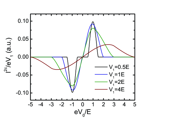
Figure 16: Second harmonic generation at zero temperature in the $\omega\tau\to\infty$ limit. The curves are plotted for different amplitudes of the excitation signal.

IV.3.4 Expansion with respect to $V_{1}$

At finite frequencies the occupation number is already time dependent ($n_{+}(t)$), thus the above considerations cannot be applied. A calculation for intermediate frequencies can be performed in the $eV_{1}\ll kT$ limit. In this case the integrals in the general solution for $n_{+}$ (Eq. 175) are calculated after expanding the coefficients $A(V_{0}+V_{1}\cos\omega t)$ and $\bar{B}(V_{0}+V_{1}\cos\omega t)$ with respect to $V_{1}$. The expansion for $A$ is:

$$A(V(t))=A_{0}+A_{0}^{{}^{\prime}}V_{1}\cos\omega t+\frac{1}{2}A_{0}^{{}^{\prime\prime}}V_{1}^{2}\cos^{2}\omega t+...$$ (198)

and similarly for $\bar{B}$. The derivatives are taken at $V=V_{0}$. In the general solution for $n_{+}$ first the quantity $e^{\int{\rm d}t\;\bar{B}(t)}$ must be calculated. The non-oscillating part of the exponent is linearly increasing with time, thus the expansion can be carried out only for the oscillating part assuming that $B_{0}^{{}^{\prime}}V_{1}/\omega\ll 1$ and $B_{0}^{{}^{\prime\prime}}V_{1}^{2}/8\omega\ll 1$:

$$e^{\int\limits_{0}^{t}{\rm d}t^{\prime}\;\bar{B}(t^{\prime})}\simeq e^{\beta t}\cdot\left(1+B_{0}^{{}^{\prime}}V_{1}\frac{\sin\omega t}{\omega}+\frac{1}{2}(B_{0}^{{}^{\prime}})^{2}V_{1}^{2}\left(\frac{\sin\omega t}{\omega}\right)^{2}+\frac{1}{4}\bar{B}_{0}^{{}^{\prime\prime}}V_{1}^{2}\frac{\sin 2\omega t}{2\omega}\right),$$ (199)

where

$$\bar{B}_{0}+\frac{1}{4}\bar{B}_{0}^{{}^{\prime\prime}}V_{1}^{2}=\beta=\frac{1}{\tau}$$ (200)

The shift of the relaxation rate by a term proportional to $V_{1}^{2}$ is due to the nonlinear behavior. The next step is to calculate the integrals $\int{\rm d}t\;A(t)e^{Q(t)}$. All the terms obtained are proportional to the exponential, $e^{\beta t}$, which is cancelled out by the factor $e^{-\beta t}$ in the expression (175). In the remaining part the higher order terms $O(V_{1}^{3})$ are dropped. The next tedious task is to collect all the terms in the coefficients of the expansion. The occupation number can be written in the following form:

$$n_{+}=n_{+}^{0}+V_{1}(n_{+}^{s}\sin\omega t+n_{+}^{c}\cos\omega t)+V_{1}^{2}(\delta n_{+}^{0}+n_{+}^{2s}\sin 2\omega t+n_{+}^{2c}\cos 2\omega t)+O(V_{1}^{3}),$$ (201)

where $n_{+}^{0}$ is the stationary occupation number at $V_{1}=0$ ($n_{+}^{0}=A_{0}/\bar{B}_{0}$), $n_{+}^{s}$ and $n_{+}^{c}$ define the amplitudes of the harmonic response to the excitation, $\delta n_{+}^{0}$ is the shift of the stationary value due to the nonlinear behavior, while $n_{+}^{2s}$ and $n_{+}^{2c}$ define the amplitudes of the second harmonic generation. The values of these coefficients are given by the following equations:

$$n_{+}^{s} = \frac{A_{0}^{{}^{\prime}}\omega^{2}+A_{0}\bar{B}_{0}^{{}^{\prime}}\beta}{\omega(\beta^{2}+\omega^{2})}-\frac{A_{0}\bar{B}_{0}^{{}^{\prime}}}{\omega\beta}$$ (202)

$$n_{+}^{c} = \frac{A_{0}^{{}^{\prime}}\beta-A_{0}\bar{B}_{0}^{{}^{\prime}}}{\beta^{2}+\omega^{2}}$$ (203)

$$\delta n_{+}^{0} = \frac{A_{0}^{{}^{\prime\prime}}}{4\beta}-\frac{A_{0}\bar{B}_{0}^{{}^{\prime\prime}}}{4\beta\bar{B}_{0}}+\frac{A_{0}(\bar{B}_{0}^{{}^{\prime}})^{2}}{2\omega^{2}\beta}-\frac{A_{0}^{{}^{\prime}}\bar{B}_{0}^{{}^{\prime}}\omega^{2}+A_{0}(\bar{B}_{0}^{{}^{\prime}})^{2}\beta}{2\omega^{2}(\beta^{2}+\omega^{2})}$$ (204)

$$n_{+}^{2s} = \frac{4A_{0}^{{}^{\prime\prime}}\omega^{2}-4A_{0}(\bar{B}_{0}^{{}^{\prime}})^{2}+A_{0}\bar{B}_{0}^{{}^{\prime\prime}}\beta+4A_{0}^{{}^{\prime}}\bar{B}_{0}^{{}^{\prime}}\beta}{8\omega(\beta^{2}+4\omega^{2})}-\frac{A_{0}^{{}^{\prime}}\bar{B}_{0}^{{}^{\prime}}\beta-A_{0}(\bar{B}_{0}^{{}^{\prime}})^{2}}{2\omega(\beta^{2}+\omega)}-\frac{A_{0}\bar{B}_{0}^{{}^{\prime\prime}}}{8\omega\beta}$$ (205)

$$n_{+}^{2c} = \frac{A_{0}^{{}^{\prime\prime}}\beta\omega^{2}-A_{0}(\bar{B}_{0}^{{}^{\prime}})^{2}\beta-A_{0}\bar{B}_{0}^{{}^{\prime\prime}}\omega^{2}-4A_{0}^{{}^{\prime}}\bar{B}_{0}^{{}^{\prime}}\omega^{2}}{4\omega^{2}(\beta^{2}+4\omega^{2})}+\frac{A_{0}^{{}^{\prime}}\bar{B}_{0}^{{}^{\prime}}\omega^{2}+A_{0}(\bar{B}_{0}^{{}^{\prime}})^{2}\beta}{2\omega^{2}(\beta^{2}+\omega^{2})}-\frac{A_{0}(\bar{B}_{0}^{{}^{\prime}})^{2}}{4\omega^{2}\beta}$$ (206)

The conditions for the expansion have excluded the narrow frequency region around $\omega=0$. Accordingly, the above results contain singular terms in $\omega$, which diverges as $\omega\rightarrow 0$. On the other hand, it has been seen that the $\omega\rightarrow 0$ limit is well defined for $n_{+}$, and indeed, it can be shown that the singular terms cancel out in the low frequency limit.

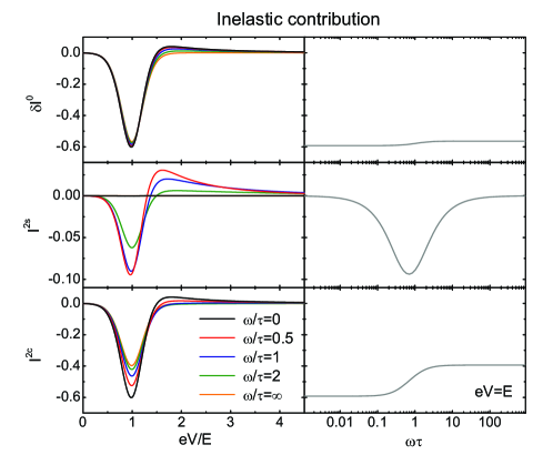
Figure 17: The left panels show the voltage dependence of DC current shift ($\delta I^{0}_{in}$) and the second harmonic terms ($I^{2s}_{in}$, $I^{2c}_{in}$) as a function of bias voltage at different excitation frequencies in the inelastic case. The right panels presents the frequency dependence of the corresponding terms at a fixed voltage of $eV=E$. The temperature is $kT=0.1E$.

The expression for the current correction can be expressed similarly to (201):

$$I=I^{0}+V_{1}(I^{s}\sin\omega t+I^{c}\cos\omega t)+V_{1}^{2}(\delta I^{0}+I^{2s}\sin 2\omega t+I^{2c}\cos 2\omega t)+O(V_{1}^{3}),$$ (207)

in the inelastic case the current correction given by Eq. (101) can be written as

$$I_{\rm in}=n_{+}D+n_{-}C=n_{+}\bar{D}+C,$$ (208)

where $\bar{D}=D-C$. These must be expanded similarly to equation (198) given for $A$. After this step the coefficients in (207) can be given as follows:

$$I_{\rm in}^{s} = n_{+}^{s}\bar{D}_{0}$$ (209)

$$I_{\rm in}^{c} = n_{+}^{c}\bar{D}_{0}+n_{+}^{0}\bar{D}_{0}^{{}^{\prime}}+C_{0}^{{}^{\prime}}$$ (210)

$$\delta I_{\rm in}^{0} = \delta n_{+}^{0}\bar{D}_{0}+\frac{1}{4}n_{+}^{0}\bar{D}_{0}^{{}^{\prime\prime}}+\frac{1}{4}C_{0}^{{}^{\prime\prime}}+\frac{1}{2}n_{+}^{c}\bar{D}_{0}^{{}^{\prime}}$$ (211)

$$I_{\rm in}^{2s} = n_{+}^{2s}\bar{D}_{0}+\frac{1}{2}n_{+}^{s}\bar{D}_{0}^{{}^{\prime}}$$ (212)

$$I_{\rm in}^{2c} = n_{+}^{2c}\bar{D}_{0}+\frac{1}{4}C_{0}^{{}^{\prime\prime}}+\frac{1}{4}n_{+}^{0}\bar{D}_{0}^{{}^{\prime\prime}}+\frac{1}{2}n_{+}^{c}\bar{D}_{0}^{{}^{\prime}}$$ (213)

These results can be analytically calculated, and for demonstration the experimentally important quantities ($\delta I^{0}$, $I^{2s}$, and $I^{2c}$) are plotted in Fig. 17. The left panels show the voltage dependence at different $\omega$ values, while the right panels demonstrate the $\omega$ dependence at the fixed bias voltage value of $eV=E$. At low frequencies, the TLS occupation number can follow the alternating voltage, thus both $I^{2c}$ and $\delta I^{0}$ are proportional to the second derivative of the $I(V)$ curve (see Eq. 172). In this limit there is no phase shift, and thus $I^{2s}=0$. In accordance with the static results, the curves show a negative peak at $eV=E$, and a positive tail at higher voltages. In the high frequency limit the TLS cannot follow the excitation, thus the occupation number sets at a constant value. Due to the intrinsic nonlinearity of the $I(V)$ curve, even in the high frequency limit a pronounced negative peak is observed at $eV=E$, but the positive background disappears. (At zero temperature the amplitude of the negative dirac delta peak at $eV=E$ in $I^{2c}$ is exactly $2/3$ times smaller in the $\omega\rightarrow\infty$ limit than in the $\omega\rightarrow 0$ limit. This factor of $2/3$ is well demonstrated by the $\omega$ dependence of $I^{2c}(eV=E)$ in Fig. 17 as well.) Around the characteristic frequency of the TLS ($\omega\tau\simeq 1$) a significant phase shift is observed, as demonstrated by the curves for $I^{2s}$.

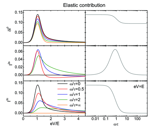
Figure 18: The left panels show the voltage dependence of DC current shift ($\delta I^{0}_{el}$) and the second harmonic terms ($I^{2s}_{el}$, $I^{2c}_{el}$) as a function of bias voltage at different excitation frequencies in the elastic case. The right panels presents the frequency dependence of the corresponding terms at a fixed voltage of $eV=E$. The temperature is $kT=0.1E$.

In the elastic case the different current components can be expressed by using Eq. (107):

$$I_{\rm el}^{s} = -(\gamma^{+}-\gamma^{-})V_{0}n_{+}^{s}$$ (214)

$$I_{\rm el}^{c} = -(\gamma^{+}-\gamma^{-})\left(n_{+}^{0}+V_{0}n_{+}^{c}\right)-\gamma^{-}$$ (215)

$$\delta I_{\rm el}^{0} = -(\gamma^{+}-\gamma^{-})\left(\frac{1}{2}n_{+}^{c}+V_{0}\delta n_{+}^{0}\right)$$ (216)

$$I_{\rm el}^{2s} = -(\gamma^{+}-\gamma^{-})\left(\frac{1}{2}n_{+}^{s}+V_{0}n_{+}^{2s}\right)$$ (217)

$$I_{\rm el}^{2c} = -(\gamma^{+}-\gamma^{-})\left(\frac{1}{2}n_{+}^{c}+V_{0}n_{+}^{2c}\right)$$ (218)

In Fig. 18 the second order terms are plotted for the elastic case. The nonlinearity of the $I(V)$ curve of the elastic contribution is basically determined by the nonlinearity of $n_{+}(V)$. Above the characteristic frequency of the TLS the occupation number cannot follow the excitation, thus both $I^{2s}_{\rm el}$ and $I^{2s}_{\rm el}$ are suppressed. The shift of the DC component ($\delta I^{0}_{\rm el}$) shows the spectroscopic peak at $eV=E$ even at $\omega\tau\to\infty$, just the amplitude is reduced by $\sim 30\%$. Around the characteristic frequency of the TLS a significant $I^{2s}_{\rm el}$ contribution is observed.

The dynamical properties of the system are also demonstrated by the phaseshift in the second harmonic contributions: $I^{2c}_{\rm el}\cos(2\omega t)+I^{2s}_{\rm el}\cos(2\omega t)=I^{(2)}\cos(2\omega t+\varphi)$. In Fig. 19 the phaseshift $\varphi$ is plotted at $eV=E$ both for the inelastic and elastic case. In the elastic contribution the phaseshift grows from $0$ to $90^{\circ}$ between the $\omega\tau\to 0$ and the $\omega\tau\to\infty$ limit. Contrary, in the inelastic case the phaseshift is zero in both limits, and even at $\omega\tau\sim 1$ a only minor phaseshift of $\sim 10\%$ is observed, as the nonlinearity is basically related to the intrinsic nonlinearity of $I(V)$ curve and the nonlinearity of $n_{+}(V)$ plays a less important role.

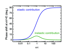
Figure 19: Phaseshift in the second harmonic current correction at $eV=E$ for the elastic and the inelastic contribution, respectively. The temperature is $kT=0.1E$.

IV.4 Conclusions

In this section the theory of the scattering on slow TLSs in point contacts was reviewed. In Sec. III.3 it was seen that the electron distribution functions and the electric potential around a ballistic contact can be determined by solving the homogeneous Boltzmann equation for a point contact geometry. The solution yields a voltage independent conductance, which is known as the “Sharvin conductance” (Eq. 63). The effect of the scattering on a slow TLS near the contact can be considered by perturbation in the collision term of the homogeneous Boltzmann equation. The electron-TLS interaction may result in backscattering processes, where an electron that has already crossed the contact is scattered back through it. These processes give a strongly voltage dependent correction to the current, for instance at zero temperature backscattering can only occur if the voltage bias exceeds the excitation energy of the TLS.

The nonlinear current correction due to the inelastic scattering of the electrons on a single TLS can be explicitly given, if the occupation number of the upper level $n_{+}$, the electron-TLS coupling strength $w$, and the geometrical factor $K_{\mathbf{R}}$ are known. It has crucial importance that the interaction of a TLS with the neighborhood is dominated by the electron-TLS scattering, and the phonon contribution is significantly smaller because of the relatively small phonon phase space at energies much smaller than the Debye energy. Therefore, the excited TLS mainly relaxes its energy through the electrons, which have a nonequilibrium distribution near the contact. As a consequence, the TLS occupation number is also not the equilibrium one, and it is strongly voltage dependent. The value of $n_{+}(V)$ can be determined by a simple dynamical equation using Fermi’s golden rule. Due to voltage dependence of $n_{+}$ a nonlinear current correction arises from the elastic scattering of the electrons on the TLS as well, provided that the scattering cross sections are different for the two states of the TLS. Both for the elastic and inelastic scattering the point contact spectrum (i.e. the second derivative of the $I-V$ curve) shows a sharp peak at the excitation energy of the TLS, and a background tail at higher voltages due to the nonequilibrium occupations.

The current correction due to the scattering on a single TLS can also be determined for a diffusive point contact. In this case the equations are more difficult, as the collision integral due to the elastic scattering on defects should also be included in the Boltzmann equation. Surprisingly, the lengthy calculations give exactly the same results as in ballistic contacts, just the geometrical prefactors are different.

The response to a time dependent bias voltage was also reviewed. Due to the nonlinearity of the $I-V$ curve the application of a small AC modulation beside the DC bias causes two important features in the response signal: (i) a second harmonic signal is generated, (ii) the average value of the current is shifted, which is referred to as the DC shift signal. If the frequency of the AC modulation is much smaller than the relaxation frequency of the TLS and its amplitude is small compared to the energy splitting, then both of these signals are proportional to the second derivative of the $I-V$ curve. On the other hand, if the modulating signal is fast compared to the relaxation of the TLS then the occupation number $n_{+}$ cannot follow the variation of the bias voltage, which has important consequences. Previously it was believed that in the high frequency limit both the elastic and inelastic contributions from the scattering on the TLS are completely suppressed in the response signal. Our more detailed calculations have shown that the DC shift signal contains a frequency independent contribution due to the rectification at voltages in the range of the TLS energies thus it is not decisive for the relaxation dynamics of the TLS. We have demonstrated that both the elastic and inelastic contributions are almost independent of the irradiation frequency in the DC shift signal. A more appropriate quantity for these studies is the second harmonic generation signal. In this case the elastic contribution is completely suppressed and the inelastic contribution shrinks by a factor of $2/3$ if the irradiation frequency exceeds the relaxation frequency of the TLS. We have also investigated the phase shift in the second harmonic signal which might be examined in subsequent experimental studies.

There is another suggestion by Kozub and RudinKozub (1997) to explain zero bias anomalies based on the adiabatic renormalization of the splitting of the TLS by electrons. That gives, however, a weak temperature dependence because the main contribution comes from the electrons far from the Fermi energy, thus that is not related to infrared singularities. The interaction between the TLS due to the Friedel oscillation was also considered and magnetic field dependence is suggested. However, it is hard to compare the theory with experiment in its present form.

It is also interesting to note that TLSs and magnetic impurities interacting with metallic electrons show several similar features. Both could lead to logarithmic corrections known as the Kondo effect. The main similarity is that the spin $S=1/2$ has also two states. Without external magnetic field or internal magnetic field characteristic to the spin glass systems the two states $S^{z}=\pm 1/2$ are degenerate, just like a TLS without splitting ($\Delta=0$). In that case the occupations of the two spin states $n_{1/2}=n_{-1/2}=1/2$ and that cannot be affected by the applied voltage on the point contact because of spin degeneracy. In Born approximation that gives a single peak at zero bias in the point contact spectra $\frac{\partial^{2}I}{\partial V^{2}}$, and no background occurs. The logarithmic Kondo corrections, however, broaden the peak which looks very similar to background in case of phonons and TLS, but that is not due to a nonequilibrium distribution.Omelyanchouk (1985) The situation is different, where the spin degeneracy is lifted by the magnetic field. In that case $n_{1/2}\neq n_{-1/2}$, thus the occupation numbers depend on the applied voltage and background occurs even without Kondo corrections.

In the following section the former experimental results are discussed and confronted with the model of slow two level systems.

V Discussion of the experimental observations

This review is aimed at collecting and summarizing the main results concerning the theory of the scattering on slow two-level systems in point contacts, and to compare those with the experiments. As a point contact probes the restricted area around the contact region, it can be used to investigate a few or even a single TLS located in the contact area. Therefore, some measurements can be directly used to study the nature of TLSs in the contact region, and to check the relevance of the model presented.

In disordered metallic point contacts TLSs with a wide variety of relaxation times can be present. A spectacular sign of the presence of TLSs in a point contact is the telegraph fluctuation of resistance, caused by defects fluctuating between metastable configurations on an experimentally resolvable timescale.Ralls (1988) Examples for such so-called two level fluctuators are shown in Fig. 20. Panel (a) shows the simplest telegraph fluctuation: the resistance is switching between two values, as discussed by considering the elastic processes (see Sec. IV.1.2), while the switching itself is an inelastic process. In panel (b) two independent telegraph fluctuations are superimposed upon each other, while on panel (c) and (d) one two-level fluctuator modulates the amplitude or the average switching time of the other. The screening of these two-level systems by electrons causes a slow-down of the TLS motion which can be described by the renormalization of the tunneling amplitude.Meisenheimer (1987); Giordano (1991) This phenomenon can be used to estimate the electron-TLS coupling constant, as it is discussed in Golding, 1992 and Zimmerman, 1991.

Figure 20: Resistance vs. time in copper nanobridges for $T<150$K showing several types of behavior. The fluctuations range from 0.005% to 0.2% of the total resistance. The time scales depend on the temperature at which the fluctuation is observed. (a) A single TLF. (b) Two independent TLFs. (c) Amplitude modulation. (d) Frequency modulation of one TLS by another. [Taken from Ralls, 1988, with kind permission of the American Institute of Physics]

This review concentrates on slow TLSs where the relaxation time is much larger than the electron-TLS interaction time, but still the TLS is fast enough not to be able to resolve it as a telegraph fluctuation of the resistance. It was seen, that such “slow” TLSs can be studied by point-contact spectroscopy, a singularity in the PC spectrum ($\partial^{2}I/\partial V^{2}$) is expected if the voltage bias coincides with the energy splitting of the TLS close to the contact. Figures 10 and 11 demonstrated that the contributions of both the elastic and inelastic scattering exhibit this anomaly at $eV=E$. In the inelastic case this anomaly always corresponds to a maximum of the differential conductance, $\partial I/\partial V$, which is reflected by a negative peak in the point contact spectrum $\partial^{2}I/\partial V^{2}$ at $eV=E$. In the elastic case a similar peak is observed, however its sign can either be negative or positive, depending on the sign of $\gamma^{+}-\gamma^{-}$ (see Eq. 107).

A similar peak is expected in the PC spectrum for fast Kondo-like TLSs, for which the electron assisted transition processes are not negligible (see Sec. II.2.2). For the fast TLSs the anomaly appears as a minimum in the differential conductance around zero bias, and the width of the zero bias minimum is determined by the Kondo temperature $T_{K}$. This feature is shown as a positive peak in the $\partial^{2}I/\partial V^{2}$ curve at $eV=kT_{K}$.Cox (1999); Ralph (1992, 1994) That peak shows very strong similarity to the Kondo peak in the presence of magnetic impurities,Yanson (1995) but no magnetic field dependence is observed, and the peak is changing by annealing.

The sign of the anomaly has crucial importance in distinguishing the slow TLSs from fast TLSs. Along this discussion the anomaly exhibiting a conductance maximum at zero bias is called “positive” zero bias anomaly (ZBA), while the conductance minimum is called “negative” ZBA. We note that the labelling of the sign of the anomaly can be confusing, as in some cases the voltage dependence of either the differential conductance or the differential resistance is plotted, in other studies the point contact spectrum is presented. Furthermore, concerning the PC spectrum, in theory the $\partial^{2}I/\partial V^{2}$ curves have direct physical meaning (showing the excitation spectrum), whereas in experimental studies usually the second derivative of the inverse curve, $\partial^{2}I/\partial V^{2}$ is plotted. Regardless of the way how the PC spectrum is plotted, the sign of the anomaly can be determined by comparing it with the sign of the contribution of the phonons. For the inelastic scattering on TLSs the increase of the bias voltages causes an enhancement of the back-scattering, thus this anomaly has the same sign as the phonon part of the spectrum. In contrast, for Kondo-like anomalies a resonant scattering is observed, which is restricted to the energy range of the Kondo temperature. In this case the back-scattering is enhanced at zero bias, and it decreases as the bias is elevated above $eV\simeq kT_{K}$, thus the anomaly has negative sign compared to the phonon contribution. In terms of this labelling, the fast TLSs should always show a negative anomaly, the inelastic contribution from slow TLSs shows up as a positive anomaly, while the elastic contribution has an indefinite sign.

In the experiments different zero bias anomalies were observed. A basic distinction should be made between the experiments performed on pure metals, and those, performed on disordered systems, like metallic glasses. In the first case the temperature dependence of the bulk resistance does not show any anomalous behavior, but due to the magnifying effect of point contacts, the scattering on a few defects near the contact might be seen in the point contact spectrum. In this case the appearance of the anomaly depends on the way the contact is created, and usually the anomaly can be destroyed by annealing. In metallic glasses, however, a high degree of disorder is initially present, and the anomalous feature seen in the PC spectrum is also reflected by the anomalous low-temperature behavior of the bulk resistivityHarris (1981) (see also Cox, 1999).

Several metallic contacts show anomalies with different signs depending on the way the contact is prepared. In the following we concentrate on a few typical and most interesting cases.

V.1 Measurements on Cu point contacts

The zero bias anomalies were widely studied in copper nanocontacts created with different methods. The first experiments by touching two Cu electrodesAkimenko (1993) reported a pronounced positive anomaly at $\simeq 1$ meV [Fig. 21a]. The ZBA has a highly asymmetric shape, which can be well fitted with the theoretical prediction for the elastic scattering on a single slow TLS. The inelastic scattering could be excluded, as in this case the anomaly should show a basically symmetric peak with a background of opposite sign [see Fig. 12]. Furthermore, as the ZBA has consequently shown a positive sign, a Kondo-like explanation could also be excluded. In some occasions further low-energy peaks were also observed [Fig. 21b], which were argued to be due to the higher excitations of the TLS.

Figure 21: (a) Point contact spectrum (curve 1) and spectral density of noise (curve 2) for a copper point contact. The circles show the theoretical prediction for the elastic scattering on a single slow TLS. The inset shows theoretical curves for the point contact spectra and the spectral density of noise. (b) Point contact spectra for copper contacts showing several low energy peaks (marked by arrows). The inset shows the possible transitions in a double-well potential leading to the peak structure observed. [Taken from Akimenko, 1993 with kind permission of Elsevier Science.]

Similar ZBAs were seen in the experiments of Keijsers et al.Keijsers (1995) on copper thin film mechanically controllable break junctions [Fig. 22a]. These samples were created by vapor deposition, and judging from the residual resistance ratio and the intensity of the phonon peaks in the PC spectrum they were of low crystalline quality implying that the contacts were in the diffusive regime. However, the authors claim that the ZBA is not due to the intrinsic disorder of the sample, but it correlates with the amount of bending and stretching of the film. In these thin film samples the ZBA has consequently shown a positive sign, and it could be well fitted with the elastic scattering on a slow TLS, similarly to the above discussed measurements of Akimentko et al.

Figure 22: (a) Point-contact spectra of copper thin-film MCB junctions with resistances 1-1.2$\Omega$, 2-22$\Omega$, 3-64$\Omega$ and 4-400$\Omega$ ($T=1.3$K). The curves have been shifted for clarity. (b) Point-contact spectrum for a Cu single crystal MCB junction ($R=30\Omega$, $T=2$K). The peaks at 17-18mV and 30mV are due to the electron-phonon interaction; the feature at bias voltages between 0 and 5mV [positive for (a), negative for(b)] is attributed to interactions between electrons and TLS. Similar anomalies were also observed in Au, Cu, Ag, and Pt contacts. [Taken from Keijsers, 1995 with kind permission of the American Institute of Physics.]

The same work of Keijsers et al.Keijsers (1995) has also presented measurements on single crystal Cu break junctions [Fig. 22b]. In this case the well resolved electron-phonon interaction spectrum implies a large elastic mean free path. In these measurements the ZBA has consequently shown a negative sign. Here, the elastic scattering on a slow TLS is still a reasonable explanation, however, the Kondo-like behavior also has to be considered.

Ralph et al.Ralph (1995) have investigated nanofabricated Cu contacts. In this case the size of the contact naturally could not be varied during the measurements, but as a great advantage, the contact was “fixed”, and thus a detailed study of the temperature and magnetic field dependence could be performed. In these experiments a well defined negative anomaly was observed if the sample was quenched [Fig. 23], and the anomaly disappeared after annealing. The detailed theoretical analysis of the curves (including scaling arguments)vonDelft (1998) has shown very good agreement with the theory of fast Kondo-like TLSs, even if their existence is still an open question.Aleiner2001a ; Aleiner2001b ; Borda (2003) The relatively high Kondo temperature ($T_{K}\sim 10$ K) can be obtained in the framework of recent theoryBorda (2003) only if the center is light (e.g. H or He) as the energy scale is the kinetic energy.Zawadowski (2004)

Figure 23: (a) Point contact spectrum for an unannealed Cu nanoconstriction. The negative zero bias anomaly at $\sim 2$ mV is attributed to the scattering on fast two level systems, while the structures at higher voltages originate from the scattering on phonons. [Taken from Ralph, 1994 with kind permission of the American Institute of Physics.] (b) Differential conductance of a Cu nanoconstriction at $T=100$ mK. The curve measured in $6$ T magnetic field is shifted down by $20\,e^{2}/h$ for clarity, and only a slight dependence on the field is observed, which supports the nonmagnetic origin of the anomaly. For comparison the inset shows the conductance of Cu constriction with $200$ ppm Mn at $100$ mK, showing a pronounced Zeeman splitting in magnetic field. [Taken from Ralph, 1992 with kind permission of the American Institute of Physics.] Similar zero bias anomaly was also observed in Ti nanojunctions.Upadhyay (1997)

In all of the above experiments the ZBAs were attributed to a single or a few TLSs. In the measurements, where consequently a positive ZBA was observed both the inelastic scattering on a slow TLS and the Kondo-like behavior can be ruled out due to shape and the sign of the anomaly, respectively. Therefore, the elastic scattering on a slow TLS remains as an explanation, which indeed gives good fit for the curves. However, it should be noted that for elastic scattering the sign of the anomaly is expected to be contact dependent. A consequent positive sign might be explained by the following argument: the atom in the higher level of the TLS can be considered to be more far away from the ordered arrangement of the atoms, thus its scattering cross section is larger than that of the low energy state, which results in an enhanced backscattering as the bias is increased.

It is interesting to note that the positive ZBAs in Keijsers, 1995 exhibit a pronounced contact size dependence: as the diameter of the junction is decreased the ZBA shifts to higher energy values [Fig. 22a]. The ZBAs showing Kondo effect in magnetically doped contacts have exhibited a similar size effect.Yanson (1995) The latter phenomenon was explained by Zaránd and Udvardi as a result of density of states oscillations nearby the surface.Zarand1996a Similar size effect is expected for the Kondo-like scattering on fast TLSs, but we stress that this explanation does not apply to the ZBAs in Fig. 22a due to the positive sign of the anomaly.

V.2 Zero bias anomalies in metallic glasses

The zero bias anomalies are also characteristic for metallic glass samples, which were always found to show negative anomalyKeijsers1996a ; Halbritter (2000) [for examples see Fig. 24] in accordance with the anomalous low-temperature increase of the bulk resistance.Harris (1981) In metallic glasses TLSs with a wide distribution of parameters can be present, thus the interpretation of the results is even more difficult. Usually the ZBA is attributed to the scattering on TLSs, however the magnetic origin also cannot be excluded. The anomalies cannot be suppressed by magnatic field in contrast to the magnetic Kondo effect, however the anomalous part of the temperature dependence of the resistance shows a small but well defined magnetoresitance, which is not present at higher temperatures.Halbritter (2000)

Another interesting feature is the telegraph fluctuation of the ZBA demonstrated by the upper curves in Fig. 24. This telegraph noise is only present in the narrow voltage region of the ZBA, that is the amplitude of the fluctuation vanishes as the voltage is increased (Fig. 25). This extraordinary behavior may be understood by assuming that a slow two level fluctuator is not directly changing the resistance (like in Fig. 20), but it is modulating the parameters of a fast TLS in the neighborhood. Therefore, the amplitude of the fluctuation only depends on the parameters of a single or a few TLSs with the slowly moving defect being in one or the other metastable position, and the contributions of electron-phonon interaction, or other TLSs being more far away from this particular defect are less significant. Comparing the voltage dependence of the fluctuation with theory, it turns out that the model of fast Kondo-like TLSs is in good agreement with the measurement, while the theory of slow TLSs gives a poor fit because of the long tail of the PC spectrum.Zarand (1998)

Figure 24: Differential resistance $R_{d}$ as a function of bias voltage for $Fe_{80}B_{20}$ (1 and 2) and $Fe_{32}Ni_{36}Cr_{14}P_{12}B_{6}$ (3) MCB junctions ($T=1.2$K). (1) A 6.6$\Omega$ contact displaying almost no noise. (2) A 366$\Omega$ contact that shows clear noise around zero bias. The noise amplitude decreases as the bias voltage increases. (3) A 145$\Omega$ contact, showing a clear two-level switching behavior between two different $R_{d}$ peaks (the time dependence of the resistance at a fixed bias shows a telegraph noise similar to those in Fig. 20). Curve 3 has been shifted for clarity. [Taken from Keijsers1996a, with kind permission of the American Institute of Physics.] The same paper has also reported about the telegraph fluctuation of the zero bias anomaly in silver break junctions. A similar telegraph fluctuation was was observed in the superconducting characteristics of Ni_xNb_1-x metallic glass break junctions.Halbritter (2000)

Figure 25: Conductance difference for mechanically controlled metallic glass break junctions. The open squares are obtained from the measured resistance change values shown in curve 3 of Fig. 24, with uncertainties of order 0.1$e^{2}/h$. The solid line is obtained from the theory of Vladár and ZawadowskiVladar1983a using a Kondo scale of $T_{K}\approx 35$K, and two different splittings for the fast TLS of $E_{1}=3.5$meV and $E_{2}=8$meV, with the assumption that the modulation by the slow center induces these two different splitting values. The other curve (filled triangles) represents another measurement from Keijsers1996a, , but in this case the theoretical fit implies that two fast TLSs are being modulated by a slow one. The inset shows conductance curves generated by the theory of Kozub and Kulik,Kozub (1986) which are also shown in Fig. 10 in the present review. [Taken from Zarand, 1998, with kind permission of the American Institute of Physics.]

V.3 High frequency behavior of the zero bias anomalies

The common feature in the yet reported ZBAs is that the anomaly appears in the voltage region $\sim 0.1-5$ mV. Usually the anomaly shows a negative sign, however even in these cases the elastic contribution from slow TLSs should be considered. A direct distinction between the fast and slow TLSs could be made by studying the relaxation dynamics of the system. In terms of the two models the position of the singularity reflects the Kondo temperature ($T_{K}$) or the energy splitting ($E$), respectively. Inserting the typical voltage range of the anomaly into the models, the standard Korringa-like relaxation rate of slow TLSs due to the creation of an electron and hole pair is $\sim 10^{-10}-10^{-7}$ s (see Eq. 174), while in the two channel Kondo model the relaxation time is in the range of $\sim 10^{-11}$s.Cox (1999) Therefore the boundary between the two cases can be investigated with microwave irradiation measurements in the GHz frequency range.

Experimentally the high frequency measurements were usually performed by irradiating the contact with a chopped microwave signal, and measuring the change of the DC current as the microwave is on and off. According to Eq. 172 the voltage dependence of the DC shift signal is proportional to the second derivative of the $I-V$ curve if the frequency of the irradiation signal is slow compared to the relaxation of the TLS, and the perturbation due to the alternating voltage is weak. Previously, it was believed that above the characteristic frequency of the TLS the DC shift signal should vanish, however the calculations were only performed for the second generation signal in the case of elastic scattering.Kozub (1986) Measurements on various systems have shown that the peak in the DC shift signal cannot be suppressed in the frequency range of the measurements ($\leq 60$ GHz).Balkashin (1998, 2001) Therefore, these studies concluded that the anomaly comes from fast TLSs with a characteristic frequency $\omega_{TLS}\gtrsim 10^{11}$ s^-1. However, according to our results in Sec. IV.3.4 these measurements are not decisive as the DC shift signal should not vanish for slow TLSs either, it should be only slightly reduced. (see upper panels in Fig. 17 and Fig. 18). The arbitrariness of the substraction of the background signal makes it even more difficult to draw a clear conclusion concerning the frequency dependence of the peak.

Figure 26: RF response signals at 60 GHz (thick solid line) and 0.6 Ghz (dashed line) and $d^{2}V/dI^{2}(V)$ dependence (thin solid line) for (a) a 26-$\Omega$ Fe₈₀B₂₀ point contact, (b) a 8-$\Omega$ Fe₇₈Mo₂B₂₀ point contact, and (c) a 15-$\Omega$ Fe₃₂Ni₃₆Cr₁₄P₁₂B₆ point contact. [Taken from,Balkashin (1998) with kind permission of the American Institute of Physics.]

More conclusive results can be obtained by measuring the second harmonic response to the high frequency irradiation, which is, however, experimentally more difficult. According to our calculations, in the second harmonic signal the peak due to the elastic scattering should disappear at high frequency, while the peak due to inelastic scattering only decreases by a factor of  2/3 (bottom panels in Fig. 18 and 17, respectively). Recent second harmonic generation measurements on Ni₅₉Nb₄₁ metallic glasses have shown,Balkashin2001b that the ZBA cannot be suppressed with frequencies up to $\sim 5$ GHz. This measurement excludes the elastic contribution of slow TLSs due to the lack of frequency dependence, and it also excludes the inelastic contribution due to slow TLSs as the sign of the peak is negative. However, the authors propose that the frequency dispersion of the smooth background signal might come from the scattering on slow TLSs.

An interesting result has been presented by Balkashin et al. on annealed Ni₅₉Nb₄₁ metallic glass samples.Balkashin (2003) The DC shift response signal was measured at various microwave irradiation frequencies both before and after annealing. The unannealed samples have shown insignificant frequency dispersion up the maximum frequency of the measurements ($\sim 5$ GHz), in agreement with the previous studies. In the annealed samples, however, the ZBA was completely suppressed at high microwave frequencies [Fig. 27]. As we have discussed, the ZBA in the DC shift response signal should not dissappear for slow TLSs either, thus the experimental observations on the annealed samples cannot be interpreted in terms of the presented theory for slow TLSs. This observation questions whether the ZBA originates from the scattering on TLSs in the studied Ni_xNb_1-x metallic glasses.

Up to now, the high frequency measurements were only performed on metallic glass samples. Unfortunately in metallic glasses various interactions coexist, which makes the interpretation of the results difficult. Especially serious problem is the normalization of the measured response signals. In pure samples the curves can be normalized to the phonon peaks, as the electron-phonon relaxation time is very small ($\tau_{\rm el-ph}\sim 10^{-13}$ s). In metallic glasses, however the phonon peaks cannot be identified, and a smooth background is observed, which can contain various contributions. In disordered systems the disorder induced electron-electron interaction (see e.g. Altshuler, 1991) and the scattering on nonequilibrium phononsKulik (1985); Yanson (1985) are also important, furthermore the scattering on a variety of TLSs with different excitation energies can also contribute to the background. Additionally, the materials under study contain magnetic ions, thus the interactions of magnetic origin also cannot be excluded. Due to the complexity of the system the background signal can also have frequency dispersion in the frequency range of the measurements, which hampers the comparison of the response signals measured at different frequencies.

A more clear picture could be obtained by investigating the high frequency behavior of the ZBAs observed in clean contacts of pure metals. In this case the ZBA is attributed to the scattering on a single or a few TLSs, and due to the ballistic nature of the contact clear phonon peaks are observed at higher energies. In this case the microwave response signals are easily compared by normalizing the curves to the phonon peaks, and thus the measurement of the second harmonic response signal provides explicit information about the relaxation dynamics of the system. Especially interesting would be the study of positive ZBAs in copper nanojunctions (or in other metals like Ag, Au and Pt), which are explained by the elastic scattering on slow TLSs.

Figure 27: Evolution of the PC spectra of a contact of the annealed alloy Ni₅₉Nb₄₁ with Ag in measurements at different frequencies: a sonic frequency (1) and microwave frequencies $\omega=$ 0.48 GHz (2), 2.036 GHz (3), and 4.72 GHz (4). The anomaly is strongly suppressed with the microwave irradiation, whereas the ZBA in unannealed samples is unaffected by the same irradiation. [Taken from Balkashin, 2003 with kind permission of the American Institute of Physics.]

V.4 Conclusions

A large variety of point contact spectroscopy measurements show ZBAs, which may be attributed to the scattering of electrons on TLSs. Certain measurements on Cu nanocontacts show positive ZBAs, which can be well explained by the elastic scattering on slow TLS. In this case, however, the reason for the consequently positive sign of the anomaly is not well understood. Another group of measurements show negative ZBAs, and among these the experiments on Cu nanocinstrictionsRalph (1995) are well interpreted in the framework of the two channel Kondo model. In these studies the ZBAs are attributed to a few or even a single TLS, which allows a direct comparison of the experimental observations with the theoretical predictions. ZBAs are frequently observed in metallic glass samples, however, in this case the complexity of the system makes the interpretation of the results more difficult. Interesting attempts were made by investigating the frequency dispersion of the ZBAs in metallic glasses, however some of the results were misinterpreted due to the lack of the theoretical calculation for the frequency dependence of the DC shift signal. Novel second harmonic generation measurements on Ni_xNb_1-x metallic glasses has proved that in this system the ZBA cannot be explained by the scattering on slow TLSs, however slow TLSs can give contribution to the background. The study of the high frequency behavior of a few TLSs near clean metallic contacts might provide a more clear information about the relaxation dynamics of TLSs.

In the cases cited above the origins of the TLSs are not well known. TLSs can occur, however, in crystalline material with deviation from the stochiometric composition or disorder as well. The TLS is formed in crystalline neighborhood where the size or the shape of the cavity in which the atom is sitting can be modified by the surroundings. In such cases clear indication of orbital Kondo effect was found in PbTe if some Pb atoms are replaced by smaller Ge atoms.Katayama (1987) However, this material is not so easy to produce in a controlled way. Recently a new family of material was discovered, which are metallic and they are composed of U, Th, As, Se and S.Henkie (2001) The systematic study of these well-controlled materials may also provide the possibility to understand the TLS-electron interaction in more detail.

VI Final remarks

The point contact spectroscopy is a very powerful method to investigate the dynamics of slow TLSs and magnetic Kondo impurities and resonances of unknown, nonmagnetic origin, presumably due to some structured defects at zero bias. That spectroscopy is complementary of tunneling spectroscopy with oxide barrierWolf (1989) or break junction in the tunneling limit,Keijsers1996b ; Keijsers (2000) but there are similarities and differences as well. The local excitations in the barrier as molecular vibrations or magnetic spin flip processes open new tunneling channels resulting in extra current at voltages above the excitation energy. That gives just the opposite sign compared to the point contact case, as those anomalies are the negative ones. The magnetic impurities in the electrodes nearby the barrier can also depress the local tunneling density of states around the Fermi level in the energy range of the Kondo temperature.Mezei (1971); Bermon (1978) That gives a negative zero bias anomaly just like in the point contact case.

In the future it would be very important to make systematic studies concerning the TLS, starting with the slow TLS with contributions of arbitrary signs due to dominating elastic processes. The detailed studies of the frequency dependence based on the theoretical part of the present review would be especially useful and that would clarify some of the contradictions of the present time.

It is very important to study further the resonances of unknown origin which have strong resemblance to nonmagnetic Kondo behaviorCox (1999) and to make attempts to determine their origin in at least a few cases.

The origin of those resonances has been the subject of theoretical debates in the recent years. Originally it was proposed that Kondo effect could arise from tunneling TLSs with non-commutative couplings e.g. due to the screening by electrons and electron assisted tunneling (see e.g. Cox, 1999). It was shown, however, that the adiabatic screening of the moving atom by electrons depresses the tunneling rate in such a strong manner,Kagan (1988, 1992); Aleiner2001a ; Aleiner2001b that the actual Kondo temperature is negligible. Recently, it has been suggested that the situation can be changed if the atom in the double potential well has the ground-state below the potential barrier, but the first excited state is above it.Borda (2003) Then this objection could be avoided, but the value of the splitting raises many questions. That theory for an intermediate heavy atom gives too small $T_{K}$, not more than $0.1-0.2$ K and that cannot explain the resonances of typical width of $10-20$ K. There is, however, the possibility of light atoms like hydrogen,Zawadowski (2004) as the dominating energy scale is the kinetic energy of the atom in the potential well. Therefore, it would be very important in the future to study hydrogen defect either in atomic states or water contamination, where the hydrogen could still change its position.

Summarizing, the origin of slow TLS and the dubious resonances deserve extended further studies.

VII Acknowledgements

We acknowledge to all the authors laying down the principles of slow TLSs in point contacts. We are especially thankful to I.K. Yanson and Sz. Csonka for the careful reading of the manuscript, and also to K.E. Nagaev, J. von Delft, J.M. van Ruitenbeek, O.P. Balkashin, A.N. Omelyanchouk, I.O. Kulik, G. Zaránd, D. C. Ralph, G. Mihály, R. A. Buhrman and H. van Kempen for their useful remarks. Part of this work was supported by the Hungarian Research Funds OTKA T026327, TS040878, T037451, T038162, T034243.

References

- Agrait (2003) N. Agrait, A. L. Yeyati, J. M. van Ruitenbeek Quantum properties of atomic-sized conductors Phys. Rep. 377 81 (2003)
- Akimenko (1993) A. I. Akimenko and V. A. Gudimenko Solid State Communications 10 925 (1993)
- (3) I.L. Aleiner, B.L. Altshuler, Y.M. Galperin Phys. Rev. B 63, 201401 (2001)
- (4) I.L. Aleiner, B.L. Altshuler, Y.M. Galperin, T.A. Shutenko Phys. Rev. Lett. 86, 2629 (2001)
- Altshuler (1991) Mesoscopic Phenomena in Solids ed. by B.L. Altshuler, P.A. Lee, and R.A. Webb, North-Holland (1991)
- Anderson (1967) P. W. Anderson, Phys. Rev. Lett. 18, 1049 (1967)
- Anderson (1972) P.W. Andreson, B.I. Halperin, C.M. Varma Phil. Mag. 25 1 (1972)
- Ashraf (1982) M. Ashraf, J.C. Swihart Phys. Rev. B. 25 2094 (1982)
- Balkashin (1992) O.P. Balkashin, Fiz. Nizk. Temp. 18 659 (Sov. J. Low Temp. Phys. 18 470) (1992)
- Balkashin (1998) O.P. Balkashin, R.J.P. Keijsers, H. van Kempen, Yu.A. Kolesnichenko, and O.I.Shklyarevskii, Phys. Rev. B 58 1294 (1998)
- Balkashin (2001) O. P. Balkashin, I. K. Yanson, A. Halbritter, G. Mihály, Solid State Commun. 118, 623 (2001)
- (12) O. P. Balkashin, I. K. Yanson, A. Halbritter, G. Mihály, Low Temp. Phys. 27, 1021 (2001)
- Balkashin (2003) O. P. Balkashin, I. K. Yanson, A. Halbritter, G. Mihály, Low Temp. Phys. 29, 123 (2003)
- Bermon (1978) S. Bermon and C.K. So, Phys. Rev. Lett. 40, 53 (1978)
- Bezuglyi (2000) E. V. Bezuglyi, A. L. Gaiduk, V. D. Fil, S. Zherlitsyn, W. L. Johnson, G. Bruls, B. Lüthi, B. Wolf, Phys. Rev B 62, 6656 (2000)
- Black (1979) J.L. Black, B.L. Györffy, J. Jäckle, Phil. Mag. B 40, 331 (1979)
- Black (1981) J.L. Black in Glassy metals I, edited by H.J. Guntherodt and H. Beck (Springer-Verlag, New-York, 1981)
- Borda (2003) L. Borda, A. Zawadowski, G. Zarand, Phys. Rev. B 68, 045114 (2003)
- (19) S.N. Coppersmith Phys. Rev. B 48 142 (1993)
- (20) S.N. Coppersmith Phys. Rev. B. 47 4922 (1993)
- Costi (1996) T. A. Costi and C. Kieffer, Phys. Rev. Lett. 76, 1683 (1996)
- Costi (1997) T. A. Costi, Phys. Rev. B 55, 3003 (1997)
- Costi (1998) T. A. Costi, Phys. Rev. Lett. 80, 1038 (1998)
- Cox (1987) D. L. Cox, Phys. Rev. Lett. 59, 1240 (1987)
- Cox (1999) D.L. Cox and A. Zawadowski, Exotic Kondo Effects in Metals, Taylor and Francis UK, 1999
- vonDelft (1998) J. von Delft, D.C. Ralph, R.A. Buhrman, A.W.W, Ludwig, V. Ambegaokar, Ann. Phys. 263, 1 (1998)
- vonDelft (1999) J. von Delft, A. W. W. Ludwig, V. Ambegaokar, Ann. Phys. 273, 175 (1999)
- Duit (1989) A. M. Duit, A. G. M. Jansenand P. Wyder, J. Phys. Cond. Matt. 1, 3157 (1989)
- Esquinazi (1998) P. Esquinazi, R. Konig in Tunneling Systems in Amorphous and Crystalline Solids, ed. by P. Esquinazi (Springer Verlag Berlin Heidelberg 1998)
- Giordano (1991) N. Giordano in Mesoscopic Phenomena in Solids, p. 131 Eds. B. L. Altshuler, P.A. Lee, and R. A. Webb. 1991 North-Holland Amsterdam.
- Grabert (1986) H. Grabert, S. Linkwitz, S. Dattagupta, U. Weiss, Europhys. Lett.2, 631 (1986)
- Golding (1973) B. Golding, J.E. Graebner, B.I. Halperin, R.J. Schutz Phys. Rev. Lett. 30 223 (1973)
- Golding (1978) B. Golding, J.E. Graebner, A.B. Kane, J.L. Black, Phys. Rev. Lett. 41, 1487 (1978)
- Golding (1992) B. Golding, N.M. Zimmerman, S.N. Coppersmith Phys. Rev. Lett. 68 998 (1992)
- Gougam (2000) A. B. Gougam, F. Pierre, H. Pothier, D. Esteve, N. Birge, J. Low Temp. Phys. 118, 447 (2000)
- Halbritter (2000) A. Halbritter, O.Yu. Kolesnychenko, G. Mihály, O.I. Shklyarevskii, H. van Kempen Phys. Rev. B 61 5846 (2000)
- Harris (1981) R. Harris and J. O. Strom-Olsen in Glassy metals II, edited by H. J. Guntherodt and H. Beck (Springer-Verlag, New-York, 1981)
- Henkie (2001) Z. Henkie, A. Pietraszko, A. Wojakowski, L. Kepiński, T. Cichorek, Journal of Alloys and Compounds 317-318, 52 (2001)
- Holm (1967) R. Holm, Electric contacts. Springer Verlag, Berlin, Heidelberg, New York 1967.
- Hunklinger (1973) S. Hunklinger, W. Arnold, S. Stein Phys. Lett. A 45 311 (1973)
- Hunklinger (1976) S. Hunklinger, W. Arnold, Physical Acoustics 12 1555 (1976) (edited by W.P. Mason, R.N. Thurston, New York: Academic Press)
- Imry (1999) Y. Imry, H. Fukuyama, and P. Schwab, Europhys. Lett. 47, 608 (1999).
- Jansen (1980) A. G. M. Jansen, A. P. van Gelder and P. Wyder, J. Phys. C 13, 6073 (1980)
- Kagan (1988) Yu. Kagan, N.V. Prokof’ev Solid State Commun. 65 1385 (1988); Sov. Phys. JETP 70 957 (1990)
- Kagan (1992) Yu. Kagan and N. V. Prokof’ev, in Quantum Tunneling in Condensed Media, edited by Yu. Kagan and A. J. Leggett (North Holland, Amsterdam, 1992)
- Katayama (1987) S. Katayama, S. Maekawa, H. Fukuyama, J. Phys. Soc. Japan 56, 697 (1987)
- (47) R.J.P. Keijsers, O.I. Shklyarevskii and H. van Kempen, Phys. Rev. Lett. 77, 3411 (1996); and ibid. 80, 1354 (1998)
- (48) R.J.P. Keijsers, O.I. Shklyarevskii and H. van Kempen, Phys. Rev. Lett. 76, 1138 (1996);
- Keijsers (1995) R.J.P. Keijsers, O.I. Shklyarevskii, H. van Kempen, Phys. Rev. B 51, 5628 (1995)
- Keijsers (1998) R.J.P. Keijsers, O.I. Shklyarevskii and H. van Kempen, Phys. Rev. Lett. 80, 1354 (1998);
- Keijsers (2000) R.J.P. Keijsers, O.I. Shklyarevskii and H. van Kempen, Phys. Rev. B 61, 7328 (2000);
- Keldysh (1964) L. V. Keldysh, Zh. Eksp. Teor. Fiz. 47, 1515 (1964) [Sov. Phys.-JETP 20, 1018 (1985)]
- Khotkevich (1995) A. V. Khotkevich, I. K. Yanson Atlas of point contact spectroscopy, Kluwer Academic Publishers, Boston, Dordrecht, London (1995)
- Knudsen (1934) M. Knudsen Kinetic Theory of Gases Methuen, London (1934)
- Kolac (1986) M. Koláč, B.S. Neganov, A. Sahling, S. Sahling, Solid State Commun. 57 425 (1986)
- Kondo (1976) J. Kondo, Physica 84B, 40 (1976)
- Kondo (1984) J. Kondo, Physica 124B, 25 (1984)
- Kondo (1988) J. Kondo Fermi Surface Effects, Tsukaba Conf. 1987 edited by J. Kondo and A. Yoshimori, Springer Verlag, Berlin Heidelberg New York, 1988
- Kozub (1986) V.I. Kozub and I.O. Kulik, Zh. Eksp. Teor. Fiz. 91 2243 (Sov. Phys. JETP 64, 1332) (1986)
- Kozub (1997) V.I. Kozub and A.M. Rudin, Phys. Rev. B 55, 259 (1997)
- Kulik (1977) I.O. Kulik, R.I. Shekhter and A.N. Omelyanchouk, Solid State Comm. 23 301 (1977)
- Kulik (1978) I.O. Kulik and I.K. Yanson, Fiz. Nizk. Temp. 4 1267 (1978) [Sov. J. Low Temp. Phys. 4, 596 (1979)]
- Kulik (1981) I.O. Kulik, R.I. Shekhter and A.G. Shkorbatov, Zh. Eksp. Teor. Fiz. 81 2126 (Sov. Phys. JETP 54, 1130) (1981)
- Kulik (1985) I.O. Kulik, Pisma Zh. Eksp. Teor. Fiz. 41 302 (Sov. Phys. JETP Lett. 41 370) (1985)
- Lee (1986) P.A. Lee, Physica 140A 169 (1986)
- Leggett (1987) A. J. Leggett, S. Chakravarty, A. T. Dorsey, M. P. A. Fischer, A. Garg and W. Zweiger, Rev. Mod. Phys. 59, 1 (1987)
- Lysykh (1980) A. A. Lysykh, I. K. Yanson, O. I. Shklyarevski and Yu. G. Naidyuk, Solid State Commun. 35, 987 (1980)
- Maxwell (1904) J. C. Maxwell, A Treatise on Electricity and Magnetism, Clarendon Press, Oxford (1904)
- Meisenheimer (1987) T. L. Meisenheimer, D. E. Beutler, N. Giordano Jpn. J. Appl. Phys. 26, 695 (1987)
- Mezei (1971) F. Mezei and A. Zawadowski, Phys. Rev. B 3, 3127 (1971)
- Morse (1953) P.M. Morse, H. Feshback, McGrow Hill Book Company Inc., New York, Toronto, London, Vol. II. Chapter 11. page 1195 (1953)
- Muller (1992) C.J. Muller, J.M. Ruitenbeek, L.J. de Jongh, Physica C 191, 485 (1992)
- Naidyuk (1982) Yu. G. Naidyuk, O. I. Shklyarevski and I. K. Yanson Fiz. Nizk. Temp. 8, 725 (1982) [Sov. J. Low Temp. Phys. 8, 362 (1982)]
- Nittke (1998) A. Nittke, S. Sahling, P. Esquinazi in Tunneling Systems in Amorphous and Crystalline Solids, ed. by P. Esquinazi (Springer Verlag Berlin Heidelberg 1998)
- Nozieres (1969) P. Nozières and C. T. Dominicis, Phys. Rev. 178, 1097 (1969)
- Omelyanchouk (1977) A.N. Omelyanchouk, I.O. Kulik, R.I. Shekhter, Pis’ma Zh. Eksp. Teor. Fiz. 25 465 (1977) [JETP Lett. 25, 439 (1979)]
- Omelyanchouk (1980) A.N. Omelyanchouk and I.G. Tuluzov Fiz. Nizk. Temp. 6, 1286 (1980) [Sov. J. Low Temp. Phys. 6, 626 (1980)]
- Omelyanchouk (1985) A. N. Omelyanchouk and I. G. Tuluzov Fiz. Nizk. Temp. 11, 388 (1985) [Sov. J. Low Temp. Phys. 11, 211 (1985)]
- Pecs (2000) Proceedings of “Size Dependent Magnetic Scattering” NATO ARW 2000 Pécs, Hungary
- Phillips (1972) W.A. Phillips J. Low Temp. Phyics 7 351 (1972)
- Pothier (1997) H. Pothier, S. Guéron, N.O. Birge, D. Esteve, and M.H. Devoret, Phys. Rev. Lett. 79, 3490 (1997)
- Ralls (1988) K.S. Ralls, R.A. Buhrman, Phys. Rev. Lett. 60, 2434 (1988)
- Ralph (1983) D. C. Ralph, PhD dissertation, Cornell University (1983)
- Ralph (1992) D. C. Ralph, R. A. Buhrman, Phys. Rev. Lett. 69, 2118 (1992)
- Ralph (1994) D. C. Ralph, A. W. W. Ludwig, J. von Delft, R. A. Buhrman, Phys. Rev. Lett. 72, 1064 (1994)
- Ralph (1995) D.C. Ralph, R.A. Buhrman, Phys. Rev. B 51, 3554, (1995)
- Rodrigo (1997) J. G. Rodrigo, F. Guinea, S. Vieira, F. G. Aliev, Phys. Rev. B 55, 14318 (1997)
- Sharvin (1965) Yu. V. Sharvin, Zh. Eksp. Teor. Fiz. 48 984 (1965) [Sov. Phys. JETP 21, 655 (1965)]
- Simonyi (1980) see e.g. K. Simonyi, Theoretische Elektrotechnik, 8. Aufl. Berlin. Dt. Verl. d. Wiss. 1980.
- Ujsaghy (2001) O. Újsághy, G. Zaránd, A. Zawadowski, Solid. State Comm. 117, 167 (2001)
- Upadhyay (1997) S. K. Upadhyay, R. N. Louie, R. A. Buhrman, Phys. Rev. B 56, 12033 (1997)
- Yamada (1985) K. Yamada, A. Sakurai and S. Miyazima, Prog. Theor. Phys. 73, 1342 (1985)
- Yanson (1974) I. K. Yanson, Zh. Eksp. Teor. Fiz. 66, 1035 (1974) [Sov. Phys. JETP 39, 506 (1974)]
- Yanson (1985) I. K. Yanson, O. P. Balkashin, and Yu. A. Pilipenko, Pisma Zh. Eksp. Teor. Fiz. 41 304 (Sov. Phys. JETP Lett. 41 373) (1985)
- (95) I. K. Yanson and O. I. Shklyarevskii, Fiz. Nizk. Temp. 12 899 (1986) [Sov. J. Low Temp. Phys. 12, 506 (1986)]
- Yanson (1995) I. K. Yanson, V. V. Fisun, R. Hesper, A. V. Khotkevich, J. M. Krans, J. A. Mydosh and J. M. van Ruitenbeek, Phys. Rev. Lett. 74, 302 (1995)
- Yanson (2001) I. K. Yanson, V. V. Fisun, J. A. Mydosh and J. M. van Ruitenbeek, Proceedings of NATO ARW 2000 at Pécs, Hungary
- vanGelder (1978) A. P. van Gelder, Sol. State Commun. 25, 1097 (1978)
- vanGelder (1980) A. P. van Gelder, Sol. State Commun. 35, 19 (1980)
- Verkin (1979) B.I. Verkin, I.K. Yanson, I.O. Kulik et al., Solid State Commun. 30 215 (1979)
- (101) K. Vladár and A. Zawadowski, Phys. Rev. B 28 1564 (1983)
- (102) , K. Vladár and A. Zawadowski, Phys. Rev. B 28 1582 (1983)
- (103) K. Vladár and A. Zawadowski, Phys. Rev. B 28 1596 (1983)
- Weiss (1999) U. Weiss, Quantum Dissipative Systems, Series in Modern Condensed Matter Physics Vol. 10 second edition, World Scientific, Singapore (1999)
- Wexler (1966) G. Wexler, Proc. Phys. Soc. 89, 927 (1966)
- Wolf (1989) E.L. Wolf, Principles of electron tunneling spectroscopy, Oxford University Press, New York, Oxford, 1989
- (107) G. Zaránd, A. Zawadowski, Phys. Rev. B 50, 932 (1994)
- (108) G. Zaránd, A. Zawadowski, Phys. Rev. Lett. 72, 542 (1994)
- (109) G. Zaránd, L. Udvardi, Phys. Rev. B 54, 7606 (1996)
- (110) G. Zaránd, L. Udvardi, Physica B 218, 68 (1996)
- Zarand (1998) G. Zaránd, Jan von Delft, A. Zawadowski, Phys. Rev. Lett. 80, 1353 (1998)
- (112) A. Zawadowski Phys. Rev. Lett. 45 211 (1980)
- (113) A. Zawadowski and K. Vladár, Solid State Commun. 35 217 (1980)
- Zawadowski (1999) A. Zawadowski, J. von Delft and D. C. Ralph, Phys. Rev. Lett. 83, 2632 (1999)
- Zawadowski (2004) unpublished
- Zeller (1971) R.C. Zeller, R.O. Pohl Phys. Rev. B 4 2029 (1971)
- Zimmerman (1991) N.M. Zimmerman, B. Golding, W.H. Haemmerle Phys. Rev. Lett. 67 1322 (1991)