Absence of an Almeida-Thouless line in Three-Dimensional Spin Glasses

Abstract

We present results of Monte Carlo simulations of the three-dimensional Edwards-Anderson Ising spin glass in the presence of a (random) field. A finite-size scaling analysis of the correlation length shows no indication of a transition, in contrast to the zero-field case. This suggests that there is no Almeida-Thouless line for short-range Ising spin glasses.

Since the work of Ballesteros et al. Ballesteros et al. (2000), there has been little doubt that a finite-temperature transition occurs in three-dimensional spin glasses iso . However, the behavior of a spin glass in a magnetic field is less well understood. In mean field theory Edwards and Anderson (1975), which is taken to be the solution of the infinite-range Sherrington-Kirkpatrick (SK) model Sherrington and Kirkpatrick (1975), an Ising system vec has a line of transitions in a magnetic field de Almeida and Thouless (1978), known as the Almeida-Thouless (AT) line. This line separates the paramagnetic phase at high temperatures and fields from the spin-glass phase at lower temperatures and fields. Although there is no change of symmetry at this transition, the relaxation time diverges (and for short-range systems so does the correlation length as we shall see). In the spin-glass phase below the AT line, there is “replica symmetry breaking” in which the free energy landscape breaks up into different regions separated by infinite barriers, and the distribution of relaxation times extends to infinity.

It is important to know whether the AT line also occurs in more realistic short-range models, since the two main scenarios that have been proposed for the spin-glass state differ over this issue. In the “droplet picture” Fisher and Huse (1986, 1987, 1988); Bray and Moore (1986) there is no AT line in any finite-dimensional spin glass. By contrast, the “replica symmetry breaking” (RSB) picture Parisi (1979, 1980, 1983); Mézard et al. (1987) postulates that the behavior of short-range systems is quite similar to that of the infinite-range SK model which does have an AT line as just mentioned. Both scenarios are illustrated in Fig. 1.

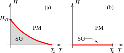
Figure 1: (a) $H$–$T$ phase diagram expected according to RSB for the short-range case. For $T<T_{\rm c}(H)$ there is a spin-glass phase (SG), whereas for $T>T_{\rm c}(H)$ the system is in the paramagnetic (PM) state. The value of the critical field at $T=0$ is called $H_{\rm AT}$. (b) $H$–$T$ phase diagram following the predictions from the droplet picture. A spin-glass phase exists only for $H=0$.

Experimentally, it has proved much more difficult to verify the transition in a field than for the zero-field transition. For the latter, the divergence of the nonlinear susceptibility gives clear experimental evidence of a transition, but unfortunately this divergence no longer occurs in a magnetic field. Experiments have therefore looked for a divergent relaxation time, and a careful analysis by Mattsson et al. Mattsson et al. (1995) finds that this does not occur in a field. However, not all experimental work has come to the same conclusion Katori and Ito (1994).

In simulations, it is most desirable to perform finite-size scaling (FSS) on dimensionless quantities for reasons that we will discuss below. One such quantity, the Binder ratio, gave some evidence for the zero-field transition Bhatt and Young (1985); Kawashima and Young (1996). However, the Binder ratio turns out to be very poorly behaved in a field Ciria et al. (1993) in short-range systems, while for the SK model it does indicate a possible transition Billoire and Coluzzi (2003a), although not with any great precision. Results of out of equilibrium simulations on large lattices in four dimensions Marinari et al. (1998a) were interpreted as evidence for RSB, although it is not completely clear that the true equilibrium behavior is probed by this procedure Barrat and Berthier (2001). By contrast, simulations Takayama and Hukushima (2004) corresponding to experimental protocols in (non-equilibrium) aging experiments have been analyzed in terms of a “dynamical crossover” consistent with the droplet picture.

Houdayer and Martin Houdayer and Martin (1999) carried out interesting calculations at $T=0$ to determine $H_{\rm AT}$, the critical field at $T=0$, see Fig. 1, for a simple cubic lattice in three dimensions. Their results indicated that $H_{\rm AT}=0$, i.e., there is no AT line, although a subsequent zero-temperature study by Krzakala et al. Krzakala et al. (2001) found some evidence of a critical field for $H\simeq 0.65$, which is much less than the “mean field” value for this lattice Pagnani et al. (2003) of around 1.86. However, Krzakala et al. Krzakala et al. (2001) could not exclude the possibility that the critical field is zero.

As noted above, the (dimensionless) Binder ratio has provided some evidence for zero-field transition at finite-$T$. However, a much sharper signature of the zero-field transition in three dimensions is provided by the correlation length Ballesteros et al. (2000) from which a dimensionless quantity is formed by dividing by the system size $L$. This approach should also provide evidence from equilibrium calculations for a transition in a field, if one occurs, and in this paper we use it to determine whether there is an AT line in a three-dimensional Ising spin glass. Our conclusion will be that there is not, at least down to fields significantly smaller than the value of 0.65 suggested by Krzakala et al. Krzakala et al. (2001).

The Hamiltonian we study is given by

$${\cal H}=-\sum_{\langle i,j\rangle}J_{ij}S_{i}S_{j}-\sum_{i}h_{i}S_{i}$$ (1)

in which the Ising spins $S_{i}=\pm 1$ lie on the sites of a simple cubic lattice of size $N=L^{3}$ ($4\leq L\leq 12$) with periodic boundary conditions, and the nearest neighbor interactions $J_{ij}$ are independent random variables with a Gaussian distribution with mean zero and standard deviation unity. At each site there is a field $h_{i}$ which, like the bonds, is randomly drawn from a Gaussian distribution, and whose mean and standard deviation are given by

$$[h_{i}]_{\mathrm{av}}=0,\qquad[h_{i}^{2}]_{\mathrm{av}}^{1/2}=H_{\rm r},$$ (2)

where $[\cdots]_{\mathrm{av}}$ denotes an average over the disorder. For a symmetric distribution of bonds, the sign of $h_{i}$ can be “gauged away” so a uniform field is completely equivalent to a bimodal distribution of fields with $h_{i}=\pm H$. Our choice of a Gaussian distribution, which still has an AT line in mean-field theory, also puts disorder into the magnitude of the $h_{i}$. We use a Gaussian distribution, rather than a uniform field, in order to apply a very helpful test for equilibration, discussed below.

To determine the correlation length we calculate the wavevector-dependent spin-glass susceptibility which, for nonzero fields, is defined by

$$\chi_{{}_{\mathrm{SG}}}(\mathbf{k})=\frac{1}{N}\sum_{i,j}\left[\Big{(}\langle S_{i}S_{j}\rangle_{T}-\langle S_{i}\rangle_{T}\langle S_{j}\rangle_{T}\Big{)}^{2}\right]_{\mathrm{av}}\!\!\!\!\!e^{i\mathbf{k}\cdot(\mathbf{R}_{i}-\mathbf{R}_{j})},$$ (3)

where $\langle\cdots\rangle_{T}$ denotes a thermal average. As in earlier work Ballesteros et al. (2000); Lee and Young (2003) the correlation length of the finite system is defined to be

$$\xi_{L}=\frac{1}{2\sin(k_{\mathrm{min}}/2)}\left[\frac{\chi_{SG}(0)}{\chi_{SG}({\bf k}_{\mathrm{min}})}-1\right]^{1/2},$$ (4)

where ${\bf k}_{\mathrm{min}}=(2\pi/L,0,0)$ is the smallest nonzero wavevector.

Now $\xi_{L}$ satisfies the finite-size scaling form

$$\frac{\xi_{L}}{L}=\widetilde{X}\left(L^{1/\nu}[T-T_{\rm c}(H_{\rm r})]\right),$$ (5)

where $\nu$ is the correlation length exponent and $T_{\rm c}(H_{\rm r})$ is the transition temperature for a field strength $H_{\rm r}$. Note that there is no power of $L$ multiplying the scaling function $\widetilde{X}$, as there would be for a quantity with dimensions. This greatly simplifies the analysis since the critical point can be seen by inspection as the temperature where data for different sizes intersect.

On the AT line, $T=T_{\rm c}(H_{\rm r})$, the “connected correlation function” $\langle S_{i}S_{j}\rangle_{T}-\langle S_{i}\rangle_{T}\langle S_{j}\rangle_{T}$ becomes long range and so, for an infinite system, the correlation length and $\chi_{{}_{\mathrm{SG}}}(0)$ diverge while for a finite system, $\xi_{L}/L$ is independent of $L$. Below the AT line, according to RSB the correlation functions no longer have a “clustering property”, i.e., $\lim_{|\mathbf{R}_{i}-\mathbf{R}_{j}|\to\infty}(\langle S_{i}S_{j}\rangle_{T}-\langle S_{i}\rangle_{T}\langle S_{j}\rangle_{T})\neq 0$, so $\chi_{{}_{\mathrm{SG}}}(0)\propto L^{d}$ and $\xi_{L}/L$ increases with $L$. Hence, according to RSB, the behavior of $\xi_{L}/L$ should be qualitatively the same as at the zero-field transition, namely it decreases with increasing $L$ above the transition, is independent of $L$ at the transition, and increases with increasing $L$ below the transition.

We use parallel tempering to speed up the simulations but unfortunately it is less efficient in a field than in zero field Moreno et al. (2003); Billoire and Coluzzi (2003b), because “chaos” with respect to a field is stronger than chaos with respect to temperature. As a result, the computer time increases very rapidly with increasing $L$, so it is unlikely that we will be able to study larger sizes in the near future without a better algorithm. In order to compute the products of up to four thermal averages in Eq. (3) without bias we simulate four copies (replicas) of the system with the same bonds and fields at each temperature.

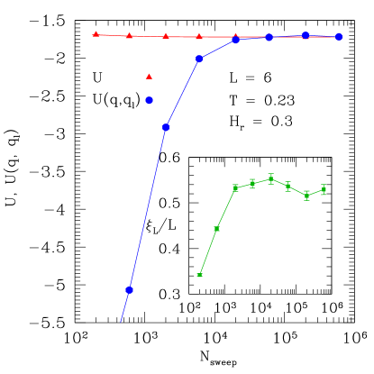
Figure 2: An equilibration plot for $L=6,H_{\rm r}=0.3,T=0.3$ showing that the data for the average energy $U$ and the quantity $U(q,q_{l})$, defined in Eq. (7), approach their common equilibrium value from opposite directions as the number of Monte Carlo sweeps $N_{\mathrm{sweep}}$ increases. The inset shows data for $\xi_{L}/L$ indicating that it has equilibrated when $U$ and $U(q,q_{l})$ have become equal.

Parameters of the simulation are shown in Table 1. Most of our work is for $H_{\rm r}=0.3$ since this is smaller than the predicted Krzakala et al. (2001); ran zero temperature value of $H_{\rm AT}=0.65$, but is not so small that the results would be seriously influenced by the zero-field transition. The lowest temperature is $0.23$ well below the zero-field transition temperature which is about Marinari et al. (1998b) $0.95$.

Table 1: Parameters of the simulations for $H_{\rm r}=0.3$. $N_{\mathrm{samp}}$ is the number of samples, $N_{\mathrm{sweep}}$ is the total number of Monte Carlo sweeps for each of the $4N_{T}$ replicas for a single sample, $T_{\rm min}$ is the lowest temperature simulated, and $N_{T}$ is the number of temperatures used in the parallel tempering method. For other values of $H_{\rm r}$, we used the same parameters but only simulated $L=4$, $6$, and $8$.

$L$	$N_{\mathrm{samp}}$	$N_{\mathrm{sweep}}$	$T_{\rm min}$	$N_{T}$
4	$5000$	$6.0\times 10^{4}$	0.23	18
6	$5319$	$6.0\times 10^{5}$	0.23	18
8	$5000$	$6.0\times 10^{5}$	0.23	18
12	$304$	$6.0\times 10^{7}$	0.23	18

For a Gaussian distributions of bonds and fields, the expression for the average energy, $U=[\langle{\cal H}\rangle_{T}]_{\mathrm{av}}$, can be integrated by parts with respect to the disorder distribution, with the result

$$U=U(q,q_{l})\,,$$ (6)

where

$$U(q,q_{l})=\frac{z}{2}\frac{q_{l}-1}{T}+\frac{q-1}{T}H_{\rm r}^{2}\,,$$ (7)

where $z$ ($=6$ here) is the number of neighbors, $q$ is the spin overlap given by

$$q=\frac{1}{N}\sum_{i=1}^{N}[\langle S_{i}^{(1)}S_{i}^{(2)}\rangle_{T}]_{\mathrm{av}},$$ (8)

and $q_{l}$ is the “link overlap” given by

$$q_{l}=\frac{2}{z}\frac{1}{N}\sum_{\langle i,j\rangle}[\langle S_{i}^{(1)}S_{j}^{(1)}S_{i}^{(2)}S_{j}^{(2)}\rangle_{T}]_{\mathrm{av}}.$$ (9)

In Eqs. (8) and (9), “$(1)$” and “$(2)$” refer to two copies of the system with the same bonds and fields. Because $U$ will decrease as the system approaches equilibrium and $q$ and $q_{l}$ will increase (since we initialize the spins in the two copies in random configurations), $U$ and $U(q,q_{l})$ approach their common equilibrium value from opposite directions and so Eqs. (6) and (7) can be used as an equilibration test. This is a generalization to finite fields of a test used previously Katzgraber et al. (2001). Figure 2 shows that these expectation are born out. We accept a set of runs as being equilibrated if $U=U(q,q_{l})$ within the error bars. The inset to the figure shows that $\xi_{L}/L$ has equilibrated when $U$ and $U(q,q_{l})$ have become equal.

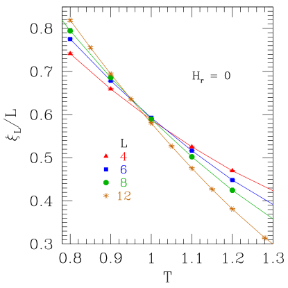
Figure 3: Data for $\xi_{L}/L$ for $H_{\rm r}=0$ for different sizes. Note that there are clear intersections at roughly a common temperature, with the data splaying out at lower temperatures. The temperature of the intersections is the zero-field transition temperature, marked $T_{\rm c}$ in Fig. 1. In this data, 5000 samples are used for the disorder average in each system size.

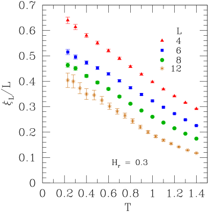
Figure 4: Data for $\xi_{L}/L$ for $H_{\rm r}=0.3$ for different sizes. Note that in contrast to the zero-field data in Fig. 3 there is no sign of intersections down to the lowest temperature $T=0.23$.

It is useful to compare results in a field with those at the zero-field transition. Hence in Fig. 3 we show data for $\xi_{L}/L$ for $H_{\rm r}=0$ for sizes up to $L=12$. For these results we set $\langle S_{i}\rangle_{T}=0$ in Eq. (3). There are clear intersections, with data splaying out at lower temperatures, indicating a transition at $T=T_{\rm c}\equiv T_{\rm c}(H_{\rm r}=0)$, in the region 0.95–1.00, in agreement with Marinari et al. Marinari et al. (1998b).

However, the analogous results for $H_{\rm r}=0.3$ shown in Fig. 4 have no sign of an intersection for sizes up to $L=12$ at temperatures down to $T=0.23$, which is considerably below the zero-field transition temperature of about 0.95. This provides quite strong evidence that there is no AT line, except possibly for fields less than $0.3$. In order to test this possibility we have also performed simulations down to $H_{\rm r}=0.05$ (for $4\leq L\leq 8$), and again found no intersections. We have also performed simulations in a uniform field, finding that data are very similar to those for the random fields, and have no intersection down to the lowest field studied, $H=0.1$.

To go to low fields without passing too close to the zero-field transition, we also tried a diagonal “cut” in the $H_{\rm r}$–$T$ plane with $H_{\rm r}/T$ kept fixed at the constant value of $0.7$. However, the equilibration problems were even more severe than for $H_{\rm r}$ fixed at 0.3, and so we have not been able to get useful data for this case.

To conclude, our finite-temperature Monte Carlo simulations provide simple, direct evidence from equilibrium calculations that there is no AT line in three dimensions. Of course, the numerical data cannot rule out a transition at exceptionally small fields, or the possibility of a crossover at much larger sizes to different behavior, but we see no particular reason for these scenarios to occur.