Effect of mesoscopic inhomogeneities on local tunnelling density of states

Abstract

We carry out a theoretical analysis of the momentum dependence of the Fourier-transformed local density of states (LDOS) in the superconducting cuprates within a model considering the interference of quasiparticles scattering on quenched impurities. The impurities introduce an external scattering potential, which is either nearly local in space or it can acquire a substantial momentum dependence due to a possible strong momentum dependence of the electronic screening near a charge modulation instability. The key new effect that we introduce is an additional mesoscopic disorder aiming to reproduce the inhomogeneities experimentally observed in scanning tunnelling microscopy. The crucial effect of this mesoscopic disorder is to give rise to point-like spectroscopic features, to be contrasted with the curve-like shape of the spectra previously calculated within the interfering-quasiparticle schemes. It is also found that stripe-like charge modulations play a relevant role to correctly reproduce all the spectral features of the experiments.

I Introduction

In the last few years scanning tunneling microscopy (STM) measurements have become a most valuable tool in investigating the physical properties of superconducting cuprates. Although, like angle-resolved photoemission spectroscopy (ARPES), this technique is mostly sensitive to the surfaces, the layered structure of the cuprates suggests that it may be representative of the bulk properties. In particular, in the recent years Fourier-transformed (FT) STM spectra showed a rich momentum structure in the local density of states (LDOS) and raised a strong debate on what elementary excitations produce such structures hoffman1 ; hoffman2 ; howald1 ; howald2 ; mcelroy ; yazdani . To be specific the dot-like patterns observed in FT-STM spectra have been attributed either to local charge-spin order with pinned static collective excitations howald2 or to interference effects between impurity-scattered quasiparticles (QP) hoffman1 ; hoffman2 ; mcelroy . Several theoretical analyses have tried so far to consider these mechanisms and to relate them to the experimental observations. Grossly speaking, it is found that pinned collective textures may account for the rather punctual (although obviously broadened) character of the LDOS patterns in momentum space polkovnikov ; zhu ; chen ; sachdev ; halperin . However, the predicted patterns show too weak an energy dependence, which contrasts with the substantial dispersion of most of the experimentally detected spots. On the other hand, the theoretical analyses based on QP interference generically produce dispersive LDOS patterns, but at a given energy the high intensity regions form extended curves in $k$ space wang ; zhang ; pereg ; capriotti , which hardly resemble the experimental spot-like intensity patterns. Moreover the STM measured dispersion curves do not properly match the ARPES-determined QP dispersions and tend to “flatten” at wave-vectors typical of charge/spin order. Finally, the weight of QP peaks in ARPES is weak and strongly depends on temperature. Therefore the QP interference effects should disappear upon approaching $T_{c}$capriotti ; kivelson . This seems to be the case for many of the structures, but experimentally it is also found that some of the k-space features persists above $T_{c}$yazdani . Therefore neither of the two pictures is fully satisfactory and one still needs to reconcile these analyses with experiments. In this paper we precisely aim to perform a systematic analysis at low temperature of the QP picture to determine whether or not physically sensible mechanisms (atomic form factors, disorder, multiple scattering, mesoscopic inhomogeneities, charge-ordering instabilities) can turn the curve-like QP spectra into more spot-like patterns. We consider the structure factors due to the short-distance structure of the Wannier orbitals, the second-order impurity scattering processes, the effect of magnetic impurities and, most importantly, the effect of mesoscopic inhomogeneities. In this way we succeed in smoothing most of the curve-like LDOS features into broad peaky structures. However, a detailed comparison of the experimental figures with our calculated spectra shows that some features cannot be properly reproduced. A better agreement is instead obtained when additional effects from charge-density modulations are considered. Therefore, our analysis shows that in the real cuprate systems there must be a coexistence between dispersive QPs (producing dispersive interference patterns broadened by inhomogeneity effects) and incipient static local charge order responsible for the enhancement of non-dispersive peaks in specific regions of the $k$ space.

The paper is organized as follows. Section II contains the model and the description of the approach. In Section III the mesoscopic inhomogeneities are introduced in the model and their effects are described. In Section IV we present our results, while our concluding remarks are contained in Section V.

II The model and the technique

II.1 The model

In STM experiments, the LDOS is measured with atomic resolution on the points ${\bf r}$ of a field of view $\ell\times\ell$ with $\ell\sim 640$Å  (several hundreds of lattice unit cells). Once the LDOS $N({\bf r},\omega)$ is obtained, its Fourier transform is a function of the momenta $(q_{x},q_{y})=(n_{x},n_{y})2\pi/\ell$, yielding the wave-vector power spectrum

$$P({\bf q},\omega)\equiv|N({\bf q},\omega)|^{2}/\ell^{2}.$$ (1)

Notice that, since the ${\bf r}$ positions of the STM scans are denser than the atomic positions, the ${\bf q}$ momenta are not restricted to the first Brillouin zone. In the following we work on an infinite lattice defined on atomic positions ${\bf R}$ (in units of the lattice spacing $a$) and use a field of view of size $L\times L$, where $L=\ell/a$. Therefore the momenta are restricted to the first Brillouin zone. This restriction is relaxed in Appendix A by including the atomic form factors encoding the orbital subatomic structure.

To consider the elastic scattering of the quasiparticles on quenched impurities, we introduce a (weak) external potential $\epsilon({\bf R})=\sum_{i=1}^{N_{i}}\epsilon({\bf R}-{\bf R}_{i})$ due to the local potential of $N_{i}$ impurities randomly located on sites ${\bf R}_{i}$ of the $L\times L=N$ two-dimensional system. Although most of the expressions below stay valid for a general form of the impurity potential, to be more specific we consider the form

$$\epsilon({\bf R})=\sum_{i}^{N_{i}}V_{0}\delta({\bf R}-{\bf R}_{i})$$ (2)

which in momentum space reads

$$\epsilon({\bf q})={V_{0}}\sum_{i=1}^{N_{i}}e^{i{\bf q}{\bf R}_{i}}$$ (3)

Aiming to perturbatively calculate the corrections induced by the impurity potential on the LDOS, we need to calculate the electron Green’s function in the superconducting state. Thus it is convenient to introduce fermionic Nambu spinors to write the Green’s functions in matrix form

$$\hat{\cal G}=\left(\begin{array}[]{cc}{\cal{G}}({\bf k},\omega)&{\cal{F}}({\bf k},\omega)\\ {\cal{F}}({\bf k},\omega)&{\cal{G}}({\bf k},-\omega)\\ \end{array}\right)$$

where the normal and anomalous Green functions are given by

$${\cal{G}}({\bf k},\omega)=\frac{\omega+\epsilon_{\bf k}}{\omega^{2}-E_{\bf k}^{2}}\;\;\;\;\;{\cal{F}}({\bf k},\omega)=\frac{\Delta_{\bf k}}{\omega^{2}-E_{\bf k}^{2}}.$$ (4)

Also the scalar (i.e., non magnetic) impurity potential can be put in matrix form

$$\hat{\epsilon}_{s}({\bf q})=\epsilon({\bf q})\left(\begin{array}[]{cc}1&\phantom{-}0\\ 0&-1\\ \end{array}\right).$$

allowing one to define the quantity

$$\Lambda_{-}({\bf q},\omega) = \int\frac{d^{2}k}{(2\pi)^{2}}\times$$

$${\cal{G}}({\bf k},\omega){\cal{G}}({\bf k}+{\bf q},\omega)-{\cal{F}}({\bf k},\omega){\cal{F}}({\bf k}+{\bf q},\omega)$$

$$= \int\frac{d^{2}k}{(2\pi)^{2}}\frac{(\omega+\epsilon_{\bf k})(\omega+\epsilon_{{\bf k}+{\bf q}})-\Delta_{\bf k}\Delta_{{\bf k}+{\bf q}}}{(\omega^{2}-E_{\bf k}^{2})(\omega^{2}-E_{{\bf k}+{\bf q}}^{2})}$$

as the $(1,1)$ element of the matrix product

$$\left(\begin{array}[]{cc}{\cal{G}}({\bf k},\omega)&{\cal{F}}({\bf k},\omega)\\ {\cal{F}}({\bf k},\omega)&{\cal{G}}({\bf k},-\omega)\\ \end{array}\right)\times$$

$$\left(\begin{array}[]{cc}1&\phantom{-}0\\ 0&-1\\ \end{array}\right)\left(\begin{array}[]{cc}{\cal{G}}({\bf k}+{\bf q},\omega)&{\cal{F}}({\bf k}+{\bf q},\omega)\\ {\cal{F}}({\bf k}+{\bf q},\omega)&{\cal{G}}({\bf k}+{\bf q},-\omega)\\ \end{array}\right).$$ (7)

The integral in Eq. (II.1) emphasizes the fact that we are working on an infinite lattice.

Since the LDOS is obtained from the imaginary part of the (1,1) element of the Green function matrix, at first order in the impurity potential, the correction to the LDOS can be written as

$$N^{(1)}({\bf R},\omega)=\Im\int\frac{d^{2}q}{(2\pi)^{2}}e^{i{\bf q}\cdot{\bf R}}\,\epsilon({\bf q})\Lambda_{-}({\bf q},\omega)$$

$$= \int\frac{d^{2}q}{(2\pi)^{2}}$$

$$\left\{\left(\epsilon^{\Re}({\bf q})\cos({\bf q}\cdot{\bf R})+\epsilon^{\Im}({\bf q})\sin({\bf q}\cdot{\bf R})\right)\,\Im(\Lambda_{-}({\bf q},\omega))\right.$$

$$+ \left.\left(\epsilon^{\Re}({\bf q})\sin({\bf q}\cdot{\bf R})+\epsilon^{\Im}({\bf q})\cos({\bf q}\cdot{\bf R})\right)\,\Re(\Lambda_{-}({\bf q},\omega))\right\}.$$

Moreover, since

$$\epsilon^{\Re}({\bf q})=\frac{1}{2}\left[\epsilon({\bf q})+\epsilon({\bf q})^{*}\right]=\frac{1}{2}\left[\epsilon({\bf q})+\epsilon(-{\bf q})\right]$$ (9)

$$\epsilon^{\Im}({\bf q})=\frac{1}{2}\left[\epsilon({\bf q})-\epsilon({\bf q})^{*}\right]=\frac{1}{2}\left[\epsilon({\bf q})-\epsilon(-{\bf q})\right]$$ (10)

then $\epsilon^{\Re}({\bf q})$ is the symmetric part of $\epsilon({\bf q})$ with respect to ${\bf q}\rightarrow-{\bf q}$ while $\epsilon^{\Im}({\bf q})$ is the antisymmetric one. Both $\Im(\Lambda_{-}({\bf q}))$ and $\Re(\Lambda_{-}({\bf q}))$ are symmetric with respect to the same transformation so the only term that survives under the sum over ${\bf q}$ is the first one in (II.1), then

$$N^{(1)}({\bf R},\omega)=\int\frac{d^{2}q}{(2\pi)^{2}}$$ (11)

$$\left(\epsilon^{\Re}({\bf q})\cos({\bf q}\cdot{\bf R})+\epsilon^{\Im}({\bf q})\sin({\bf q}\cdot{\bf R})\right)\,\Im(\Lambda_{-}({\bf q},\omega))$$

If there is inversion symmetry (for example one symmetric impurity at ${\bf R}=(0,0)$) so that $\epsilon({\bf R})=\epsilon(-{\bf R})$ then $\epsilon^{\Im}({\bf q})=0$ and $\epsilon({\bf q})=\epsilon^{\Re}({\bf q})$ and one simply has

$$N^{(1)}({\bf R},\omega)=\int\frac{d^{2}q}{(2\pi)^{2}}\epsilon({\bf q})\cos({\bf q}\cdot{\bf R})\,\Im(\Lambda_{-}({\bf q},\omega))$$ (12)

For $N_{i}$ delta-like impurities one has

$$\epsilon^{\Re}({\bf q})={V_{0}}\sum^{N_{i}}_{i=1}\cos({\bf q}\cdot{\bf R}_{i})$$ (13)

$$\epsilon^{\Im}({\bf q})={V_{0}}\sum^{N_{i}}_{i=1}\sin({\bf q}\cdot{\bf R}_{i})$$ (14)

where ${\bf R}_{i}$ are random positions.

It is worth noticing that in this scheme the LDOS $N({\bf R},\omega)$ is calculated for a fixed configuration of disorder (i.e. of impurities) and no average over these configurations is taken. Furthermore we neglect the contributions from impurities that are outside the field of view. This results in Fourier-transformed scattering potentials $\epsilon({\bf q})$, which could be sizably (and randomly) momentum-dependent. Only owing to the rather large size of the $L\times L$ field of view and to the self-averaging character of this disordered system, the $\epsilon({\bf q})$ functions turn out to be sufficiently smooth to preserve the momentum structure of the $\Im(\Lambda_{-}({\bf q},\omega))$ encoding the interference effects of the scattered QP’s. In particular for an infinite system one would obtain $|\epsilon({\bf q})|^{2}/N\approx\langle|\epsilon({\bf q})|^{2}\rangle/N=n_{i}V_{0}^{2}$ (where the angular brackets denote disorder average)capriotti . One could also calculate the LDOS power spectrum by Fourier transforming the LDOS correlation function $\langle N({\bf R},\omega)N(0)\rangle$. Again, this procedure would only allow to extract informations on the momentum structure of $\Lambda({\bf q})$ if carried out on sufficiently large grids such that the resulting $\epsilon({\bf q})$ is smooth.

We consider a system with a bare tight-binding band $\epsilon_{k}=-2t(\cos k_{x}+\cos k_{y})-4t^{\prime}\cos k_{x}\cos k_{y}-\mu_{0}$ ($t$ and $t^{\prime}$ are the nearest-neighbor and the next-nearest-neighbor hopping parameters on a square lattice and $\mu_{0}$ is the chemical potential) and a $d$-wave superconducting gap $\Delta_{k}=\Delta_{0}(\cos k_{x}-\cos k_{y})/2$. In this way the QP dispersion is $E_{\bf k}=\sqrt{\epsilon_{\bf k}^{2}+\Delta_{\bf k}^{2}}$. To compare our results with the experiments of Refs. hoffman1, ; hoffman2, ; mcelroy, we take the following parameter values, which, for $t\approx 150\,meV$ are suitable for a ${\rm Bi_{2}Ca_{2}SrCu_{2}O_{8+x}}$ sample around optimal dopingnorman : $t^{\prime}=-0.3t,\,\,\,\Delta_{0}=0.25t=37.5\,meV$. For the sake of definiteness we take the doping $x=0.15$, for which we calculate the chemical potential to be $\mu_{0}=-1.0t$.

Fig. 1 displays the momentum dependence of the LDOS for this system and well reproduces typical results of Ref. Capriotti et al.capriotti . To make the comparison with figures reported in experimental papers, throughout this paper we will mark as darker the regions with larger spectral intensity. Moreover, we orientate the momentum axes in such a way that the Cu-O directions (usually taken as the $x=(1,0)$ and $y=(0,1)$ directions in theoretical papers) here are taken along the diagonals of the figures. Notice also that, with the chosen orientation, the second Brillouin zone is visible in our figures.

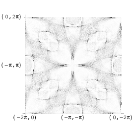
Figure 1: Momentum-dependent LDOS for an homogeneous ${\rm Bi_{2}Ca_{2}SrCu_{2}O_{8+x}}$ superconducting system with $x=0.15$. The momenta are in units of the inverse lattice spacing. To facilitate the comparison with experiments in this and subsequent figures we rotate the Brillouin zone so that the Cu-O directions of the square $CuO_{2}$ planes are along the diagonals of the figure. The tight-binding parameters are ($t=150\,meV$) $t^{\prime}=-0.3t;\,\,\mu_{0}=-1.0t\,;\,\,\Delta_{0}=0.25t=37.5\,meV$, $\omega=-0.08t=-12\,meV$. The concentration of impurities is $1\%$.

The spectrum in Fig. 1 has been discussed in terms of the constant-energy curves of the quasiparticle dispersion relation $E_{{\bf k}}$. Fixing the $E_{{\bf k}}$ identifies “banana” shaped curves in momentum space with large density of states at the extremitiesmcelroy ; capriotti .

These spectra are quite different in various respects from the experimental ones. It is apparent that the high-intensity regions are extended lines, which do not reproduce the spot-like shape of the experimental high-intensity regions. One can show that large contributions to the spectra are obtained when both denominators in Eq. II.1 are small. Extended one-dimensional features are obtained when a translation of ${\bf q}$ of one banana makes it tangent to another banana. Changing ${\bf q}$ keeping the two bananas tangent defines a one-dimensional feature of high intensity. Crossing of two of these features produces a high intensity spot. However those spots are quite different from the experimental ones since they are clearly associated with the one-dimensional crossings.

Another important difference is that there is no intensity around zero momentum. This lack of spectral weight in the ${\bf q}=(0,0)$ region contrasts with the presence of rather intense broad peaks appearing in the experimental data.

Finally, the theoretical treatment considers a mesh coincident with the atomic positions and correctly reproduces a spectrum, which is periodic in momentum space: $N({\bf q},\omega)=N({\bf q}+{\bf G},\omega)$ with ${\bf G}$ a reciprocal lattice vector. However, this feature is not present in the experimental spectra, where the peaks in the second Brillouin zone are suppressed with respect to their first Brillouin zone partners. The presence of these form factors is easily accounted for by the local space structure of the Wannier orbitalshalperin and this effect is described in Appendix A. As shown in Fig. 2, the introduction of Wannier orbitals does not significantly improve the unrealistic appearance of the spectrum. This is most evident at low momenta, where the non-point-like nature of the orbitals is obviously immaterial.

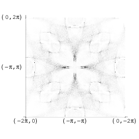
Figure 2: Momentum-dependent LDOS spectra for a system with the same parameters as in Fig. 1 and Gaussian Wannier orbitals with width ${\sigma}=0.0625$ in units of square lattice spacing. The impurity concentration is $1\%$ and the spectrum is taken at $\omega=-0.08t=-12\,meV$.

In the next Sections, we will elaborate on the above expressions to consider the inhomogeneous distribution of doping and the consequent inhomogeneous distribution of the chemical potential and of the superconducting gap.

III Effect of Mesoscopic inhomogeneities

STM experiments show large fluctuations in the gap amplitude over large length scales pan ; lang . It is quite important to recognize that the size of these regions is of several unit cells, $\xi\approx 13-15A$, and is apparently unrelated with the average distance between impurities.

Competition among different phases in strongly correlated systems can give rise to mesoscopic inhomogeneitieslor01I ; lor01II ; lor02 . One can expect that this effect is enhanced by the inhomogeneous distribution of the doping. Here we will not discuss the microscopic mechanisms that can give rise to this effect but consider it as granted and we analyze the consequence on the LDOS.

Since the mesoscopic inhomogeneities involve several unit cells and differences can be substantial from one region to the other we choose an approach, which is analogous to the usual semiclassical treatment of electrons in presence of slowly varying perturbations, where the electron distribution depends both on space and momenta. In the same spirit we allow the Green functions to depend parametrically on the real-space region of the sample via the space dependence of both the chemical potential $\mu=\mu({\bf R})$ and the superconducting (SC) gap $\Delta=\Delta({\bf R})$. This gives rise to a local density of states which depends explicitly on ${\bf R}$ due to the conventional impurity scattering, and implicitly trough the parametric dependence of the gap and the chemical potential.

$$N({\bf q},\omega) = \sum_{{\bf R}}e^{-i{\bf q}{\bf R}}N(\Delta({\bf R}),\mu({\bf R}),{\bf R},\omega)$$ (15)

Here the sum is restricted to the $L\times L$ field of view and the first order expression of $N(\Delta({\bf R}),\mu({\bf R}),{\bf q},\omega)$ is given by Eq. II.1 but with the Green functions computed with the local value of $\mu({\bf R})$ and $\Delta=\Delta({\bf R})$. For example ${\cal{G}}$ is given by Eq.(4), but with

$$\epsilon_{k} = -2t(\cos k_{x}+\cos k_{y})-4t^{\prime}\cos k_{x}\cos k_{y}-\mu({\bf R})$$

$$\Delta_{k} = \Delta({\bf R})(\cos k_{x}-\cos k_{y})/2$$

These expressions introduce a parametric dependence of ${\cal G}$ on the position ${\bf R}$ via the local values of the chemical potential and of the maximum value of the $d$-wave SC gap $\Delta_{0}$ (however, to keep the notations simple, in the following we often do not explicitly indicate this $R$ dependence). This approach allows for substantial differences in the gap and local chemical potential from one region to the other and hence go beyond conventional perturbative formulations.

To realize a specific inhomogeneous distribution of $\mu$ and $\Delta$ we consider space fluctuations of the doping around a given average value $x$. Specifically we generate an inhomogeneous map characterized by doping fluctuations of 30% (i.e. $x=x({\bf R})$ locally ranges from $0.1$ to $0.2$) of typical size $\xi\sim 3-4$ lattice units. We take this range of fluctuations as an estimate deduced from the (larger) relative fluctuations of the gap observed in the ${\rm Bi_{2}Ca_{2}SrCu_{2}O_{8+x}}$ sample of Ref. pan, and under the assumption that the gap and the doping are linearly related. For simplicity the smooth map was replaced by a mesa like function by determining contour levels of the smooth map and assigning to all points between two successive contour levels a constant doping equal to the average value of the two limiting contours. In this way the doping interval was (arbitrary) coarse-grained in five slices and for each of the five possible doping values the corresponding values of the chemical potential and of the SC gap where calculated. In particular, starting from the given tight-binding structure, the chemical potential was determined according to the local doping $x({\bf R})$, while for simplicity the maximum value of the $d$-wave gap was determined by a linear rescaling with doping. The resulting coarse-grained map is shown in Fig. 3 for a $200\times 200$ field of view. A direct comparison shows a close resemblance between our space inhomogeneity map and the similar experimental figures of Refs. pan, ; lang, .

III.1 Zeroth order

Even in the absence of impurity scattering, the inhomogeneities on the chemical potential and on the SC gap affect the LDOS spectra. In particular if $\xi$ is the typical size of the domains in which $\mu$ and $\Delta$ can be taken as nearly constant, it is quite natural to expect that a broadening of the spectra is obtained around the $q=(0,0)$ wave-vector, over a k-space range of the order of $\xi^{-1}$. Specifically,

$$N^{(0)}({\bf q},\omega) = \sum_{{\bf R}}e^{-i{\bf q}{\bf R}}N^{(0)}(\Delta({\bf R}),\mu({\bf R}),\omega)$$ (17)

$N^{(0)}(\Delta({\bf R}),\mu({\bf R}),\omega)$ is the LDOS without impurities for a (homogeneous) system with SC gap $\Delta({\bf R})$ and chemical potential $\mu({\bf R})$:

$$N^{(0)}(\Delta({\bf R}),\mu({\bf R}))=-\frac{1}{\pi}\Im\int{\frac{d^{2}q}{(2\pi)^{2}}{\cal G}(\Delta({\bf R}),\mu({\bf R}),{\bf q},\omega)}$$

where the Green function is taken in the absence of impurity scattering and is given by the same expression of Eq.(4), but with space-dependent parameters $\mu({\bf R})$ and $\Delta({\bf R})$.

The numerical evaluation of $N^{(0)}({\bf q},\omega)$ [Eq. (17)] for the specific distribution of inhomogeneities shown in Fig. 3 (upper panel), indeed produces a rather strong peak around zero momentum (Fig. 3, lower panel). This effect can be simply understood as follows. The inhomogeneities in $\Delta({\bf R})$ and $\mu({\bf R})$ reflect in the DOS, which deviates from its average value $N_{0}$. For illustrative purpose, we consider an approximate linear dependence of the DOS from the energy in the nodal approximation, so that, for small deviations of $\Delta$ and $\mu$ we find

$$N(\Delta({\bf R}),\mu({\bf R}))=N_{0}(\omega)\left[1+\frac{\Delta({\bf R})-\Delta_{0}}{\Delta_{0}}+\frac{\mu({\bf R})-\mu_{0}}{\mu_{0}}+...\right]$$ (18)

Here $\Delta_{0}\equiv\langle\Delta({\bf R})\rangle$ and $\mu_{0}\equiv\langle\mu({\bf R})\rangle$ are the average values of $\Delta$ and $\mu$ respectively. We also assume a Gaussian distribution

$$P_{X}({\bf R})={\cal N}e^{-\left[\xi^{2}|\nabla X({\bf R})|^{2}+X({\bf R})^{2}\right]/A}$$ (19)

where $A$ is suitably chosen to give the expected size of the fluctuations of about thirty per cent. Here $X({\bf R})=\delta\Delta({\bf R}),\,\delta\mu({\bf R})$, with $\delta\Delta({\bf R})\equiv\Delta({\bf R})-\Delta_{0}$ and $\delta\mu({\bf R})\equiv\mu({\bf R})-\mu_{0}$. The LDOS correlation function then takes the form

$$\langle N(\Delta({\bf R}),\mu({\bf R}))N(\Delta(0),\mu(0))\rangle=$$

$$N_{0}^{2}(\omega) \left[1+\frac{\langle\delta\Delta({\bf R})\delta\Delta(0)\rangle}{\Delta_{0}^{2}}+\frac{\langle\delta\mu({\bf R})\delta\mu(0)\rangle}{\mu_{0}^{2}}+...\right],$$

Taking the Fourier transform, one obtains the LDOS power spectrum

$$P({\bf q},\omega)=N_{0}(\omega)\left[\frac{A}{\xi^{2}|{\bf q}|^{2}+1}+\frac{A}{\xi^{2}|{\bf q}|^{2}+1}...\right].$$ (21)

Therefore the $\mu$ and $\Delta$ distributions generate the peak around ${\bf q}=(0,0)$ in the figures reported in the next subsections. As expected, we find that the width of this peak scales as $\xi^{-1}$ showing that this simple effect explains the central bump, which is not reproduced in the usual “homogeneous” approaches.

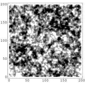
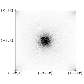
Figure 3: Upper panel: Real-space map of a $200\times 200$ field of view with randomly distributed regions of tipical size $\xi\approx 3.5$ (in units of lattice spacing) and five different values of doping and corresponding values of gap and chemical potential (see text). Lower panel: Momentum-dependent LDOS without impurity scattering as it arises from Eq. (17) with the mesoscopic distribution of Fig. 3 (upper panel).

III.2 First order

Besides the above simple zero-th order effect, the local inhomogeneities affect the first-order corrections induced by the scattering of the QP on the random impurities. Therefore, in the presence of the mesoscopic inhomogeneities, we recalculate the first-order corrections to the LDOS

$$N^{(1)}({\bf q},\omega)=-\frac{1}{\pi}\sum_{\bf R}e^{-i{\bf q}\cdot{\bf R}}\,\Im\left[\int\frac{d^{2}q^{\prime}}{(2\pi)^{2}}e^{i{\bf q}^{\prime}\cdot{\bf R}}\epsilon({\bf q}^{\prime})\Lambda_{-}({\bf q}^{\prime},\omega)\right]$$ (22)

where $\Lambda_{-}({\bf q},\omega)$ has the same form as in Eq. (II.1), but with $R$-dependent normal and anomalous Green functions according to their parametric dependence on $\Delta({\bf R})$ and $\mu({\bf R})$. The sum over ${\bf R}$ is to be intended over the points of the $L\times L$ grid of the field of view. We also consider the possibility of QP’s scattering on magnetic impurities, for which the matrix representation is given by

$$\hat{\epsilon}_{m}({\bf q})=\epsilon_{m}({\bf q})\left(\begin{array}[]{cc}1&\phantom{-}0\\ 0&\phantom{-}1\\ \end{array}\right)$$

In the case of magnetic impurity scattering, the expression of $\Lambda$ for the LDOS of a spin-up electron reads

$${\Lambda_{+}}({\bf q},\omega)=\int\frac{d^{2}k}{(2\pi)^{2}}$$

$${\cal{G}}_{R}({\bf k},\omega){\cal{G}}_{R}({\bf k}+{\bf q},\omega)+{\cal{F}}_{R}({\bf k},\omega){\cal{F}}_{R}({\bf k}+{\bf q},\omega)$$

$$=\int\frac{d^{2}k}{(2\pi)^{2}}\frac{(\omega+\epsilon_{\bf k})(\omega+\epsilon_{{\bf k}+{\bf q}})+\Delta_{\bf k}\Delta_{{\bf k}+{\bf q}}}{(\omega^{2}-E_{\bf k}^{2})(\omega^{2}-E_{{\bf k}+{\bf q}}^{2})},$$ (24)

Since an overall minus sign is obtained for spin-down electrons, no contribution is obtained at first order for the total LDOS in the case of magnetic impurities.

III.3 Second order

At second order in the impurity concentration, if we consider only scattering processes that occur on the same site, we have

$$N^{(2)}({\bf q},\omega)=-\frac{1}{\pi}\sum_{R}e^{-i{\bf q}{\bf R}}\times$$ (25)

$$\Im\left\{\int\frac{d^{2}p}{(2\pi)^{2}}e^{i{\bf p}{\bf R}}\left[\Sigma_{1}({\bf p},\omega)\Lambda_{-}({\bf p},\omega)+\Sigma_{2}({\bf p},\omega){\Lambda_{+}}({\bf p},\omega)\right]\right\}$$

where

$$\Sigma_{1}({\bf p},\omega) = \left(\epsilon^{2}({\bf p})+\epsilon_{m}^{2}({\bf p})\right)\sum_{\bf k}\frac{\epsilon_{\bf k}}{\omega^{2}-E_{\bf k}^{2}}$$ (26)

$$\Sigma_{2}({\bf p},\omega) = \left(\epsilon^{2}({\bf p})+\epsilon_{m}^{2}({\bf p})\right)\sum_{\bf k}\frac{\omega}{\omega^{2}-E_{\bf k}^{2}}$$ (27)

and $\Lambda_{\pm}$ are given by Eq.(II.1) and Eq.(24) respectively.

Various observations are in order here. First of all it is found that at second order, a finite contribution to the LDOS in momentum space is obtained also in the case of magnetic scattering. Notice also that, contrary to the first-order case, the real parts of $\Lambda_{-}$ and ${\Lambda_{+}}$ both contribute to the LDOS. Finally we notice from Eqs. (25)-(27) that second-order QP interference processes may contribute to the LDOS at zero momentum $N({\bf q}=(0,0))$. This contribution adds to the zeroth-order peak arising from the mesoscopic inhomogeneities described in Sec. III.B and may be present even in the absence of such inhomogeneities. This can be seen by taking $\mu({\bf R})=\mu_{0}$ and $\Delta({\bf R})=\Delta_{0}$.

Although at ${\bf q}=(0,0)$, the first-order contribution to $\Lambda_{-}(0)$ is small [see Fig. 4 (upper panel) and Appendix B], $\Lambda_{+}(0)$ does not vanish and contributes to $N^{(2)}(0)$ (both in the absence and in the presence of magnetic scattering). Therefore second-order scattering processes could contribute to the intense (rather broad) peak experimentally obtained for $N({\bf q},\omega)$ at ${\bf q}=(0,0)$. However, we checked from the relative intensity of the peaks at finite momenta that the scattering processes are weak and the second-order processes are not strong enough to explain the rather large intensity of the peak at ${\bf q}=(0,0)$. This strongly indicates that the zero-order contribution from the mesoscopic inhomogeneities is the main source of the large intensity of the zero-momentum peaks in the experiments.

IV Microscopic Spatial charge modulations

The observation (see below) that calculations of the STM spectra in terms of interfering scattered quasiparticles do not account for the observed weight of some specific spectral features motivated a further enrichment of our treatment. Specifically we considered a physically different effect arising from microscopic charge modulations. Since long time it has been suggested that the superconducting cuprates might be close to an instability leading to the spatial orderingreferenzestripes likely in the form of fluctuating onedimensional charge textures (the so-called stripes), which can even acquire a slow critical dynamics CDG around optimal doping and above. The scale of these textures is of a few lattice spacing thus we call them “microscopic” as opposed to the mesoscopic inhomogeneities consider above. The proximity to the microscopic instability can naturally reflect itself in a large enhancement of the charge susceptibility at specific wave-vectors ${\bf Q}_{ch}$ (obviously corresponding to the charge order) and to related structures in the momentum-dependent dielectric function. In particular, it is natural that the external potential introduced by static impurities is substantially screened by the nearly unstable electron liquid and acquires some structure in its momentum dependence. One can see that close to the charge instability, the static charge susceptibility acquires a nearly polar formnotaperiodicity

$$\chi({\bf q})=\frac{\chi_{0}({\bf q})}{1-V({\bf q})\chi_{0}({\bf q})}\propto\frac{\chi_{0}({\bf q})}{|{\bf q}-{\bf Q}_{ch}|^{2}+\xi_{ch}^{-2}}$$ (28)

where $\xi_{ch}$ is the correlation length for charge fluctuations. Once this charge susceptibility is introduced in the dielectric constant, one finds that the impurity potential is screened as

$${\tilde{V}}_{0}({\bf q})=V_{0}\left(1+\sum_{Q_{ch}}\frac{1}{(|{\bf q}-{\bf Q}_{ch}|^{2}+\xi^{-2}}\right).$$ (29)

For simplicity, we assume here $V_{0}\chi_{0}({\bf q}={\bf Q}_{ch})\sim 1$ and we take $\xi_{ch}^{-1}=0.25$ inverse lattice spacing. This screening gives rise to a strongly momentum-dependent impurity potential. Quite obviously, once this screened impurity potential is inserted in the expressions for $N({\bf q},\omega)$, it will filter the momentum dependence of the LDOS emphasizing the intensity at ${\bf q}\approx{\bf Q}_{ch}$.

V Results

We here describe the effects in the calculated momentum-dependent LDOS arising from the progressive introduction of the mesoscopic inhomogeneities and of the spatial charge modulations according to the scheme described in Section III and IV. To compare with the results reported in Figs. 1 and 2 for an homogeneous system, we keep considering the tight-binding model with the same parameters. Again the value of $\mu_{0}$ corresponds to a doping $x=0.15$. Besides the previously considered effect of the local Wannier structure of the orbitals, we introduce a random inhomogeneous (mesoscopic) doping distribution according to the scheme of Subsection III.A. Fig. 4 represents a momentum-space LDOS including up to second-order scattering. As it can be clearly seen, the space inhomogeneity is quite effective in modifying the STM spectra (a) by introducing substantial spectral weight around zero momenta, and (b) by broadening the curve-like spectral features. In particular, these latters acquire a “fuzzier” appearance, which emphasizes the regions of stronger intensity thereby producing more spot-like features and rendering the calculated spectra closer to the experimental data. We also notice that this effect arises from the disorder in gap and chemical potential and is therefore physically quite different from (and its effects quite more pronounced than) the impurity disorder considered in the appendix of Ref. capriotti, .

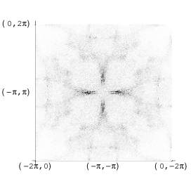
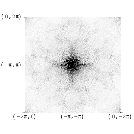
Figure 4: Upper panel: First-order-only contribution to the momentum-dependent LDOS spectra for a system with the same parameters as in Fig. 1 and 2 (Wannier orbitals are also considered). The chemical potential and the SC gap are randomly distributed according to the real-space map of Fig. 3 (upper panel). The impurity concentration is $1\%$ and the spectrum is taken at $\omega=-0.08t=-12\,meV$. Lower panel: Momentum-dependent LDOS spectra with the impurity scattering calculated including the zeroth, first and second order with $\epsilon=0.8t$. All other parameters are the same as in the upper panel,

Despite this substantial improvement, a closer comparison with the data of Refs. hoffman2, and mcelroy, (cf. Fig. 5 (lower panel) shows that the calculations of Fig. 4 fail in reproducing some of the rather intense features experimentally detected. Specifically, strong spectral features are observed along the Cu-O-Cu directions (i.e. along the diagonals of Figs. 4 and 5, see the experimental intensities schematically reported in Fig. 5, lower panel) at wave-vectors corresponding to a four-unit-cell modulation $|{\bf q}|=0.25\times(2\pi/a_{0})$ ($a_{0}$ is the lattice unit in the supposedly square $CuO_{2}$ planes) howald0 ; howald2 ; mcelroy , which are to weak in Fig. 4 (lower panel). Therefore, following the scheme of Section IV, we consider the effects of screening on the impurity potential. According to the suggestion that the cuprates are close to a charge instability, this screening is taken to be strongly momentum dependent, as a result of the strong charge susceptibility of the electron liquid at momenta ${\bf q}\approx{\bf Q}_{ch}$. The resulting calculated spectrum is reported in Fig. 5 (upper panel), where the too weak peaks in the $(\pm 1,0),(0,\pm 1)$ directions (along the diagonals of the figures) are now strongly enhanced. The comparison with experimental intensities is more direct in Fig. 5 (lower panel), where we use dots to depict the regions where experimental spectra display the strongest features. It is clear that the effect of momentum-dependent screening on the impurity potential is substantial and important to correctly reproduce all the experimental structures.

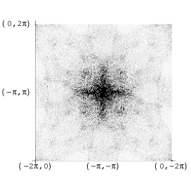
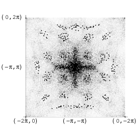
Figure 5: Upper panel: Momentum-dependent LDOS spectrum including the effects of mesoscopic inhomogeneities and the impurity scattering up to second order with $\epsilon=0.8t$. We also considered a momentum-dependent screened impurity potential according to Eqs. (29) and . (29) with $\xi_{ch}^{-1}=0.25$ in units of inverse lattice spacing. The impurity concentration is $1\%$ and the spectrum is taken at $\omega=-0.08t=-12\,meV$. Lower panel: same as in the upper panel, but with the addition of dots marking intense features in the experiments of Ref. mcelroy,

VI Conclusions

The results displayed in the previous sections allow to draw some general conclusions concerning the mechanisms leading to the formation of (point-like) structures in the LDOS as obtained in Fourier-transformed STM spectra.

First of all, disregarding the zero-order inhomogenity effects acting at low momenta, we considered the intensity of the finite-momentum peaks. From the comparison of the first and second-order contributions with experimental spectra, we can draw the conclusion that the QP scattering due to impurities is rather weak. Therefore our perturbative approach is appropriate and the first-order processes already account well for the part of the spectra, which can be attributed to the QP interference. When this mechanism at first order fails in reproducing the all relevant features of the spectra, the second-order processes do not substantially improve the calculations. The same holds true as far as the inclusion of magnetic impurities is concerned. We also took in consideration the extended character of the Wannier orbitals, which partially modifies the spectra at large wave-vectors accounting for the weakening of the spectral features at large momenta. Nevertheless the calculated spectra preserve their unrealistic features.

A substantial improvement in the theoretical calculation is represented by the inclusion of space inhomogeneities both in the SC gap and in the chemical potential as arising from doping inhomogeneities. As far as the impurity scattering is concerned, the main effect of inhomogeneities is to blur the curve-shaped spectral features promoting a more point-like appearance of the high intensity regions of the spectra. This is quite easily interpreted in terms of the (by now) standard arguments related to the relevance of some specific wave-vectors joining the parts of the electronic (d-wave gapped) spectra at fixed energy bias (see, e.g., Fig. 1 of Ref. mcelroy, ). The contours of constant-energy in the quasiparticle spectra have the well-known “banana” shape and in the absence of disorder the momentum space regions with large intensity are extended curves. However, by introducing local gap fluctuations, the length of the “bananas” fluctuates, while the transversal, i.e. the width, fluctuations of the “bananas” are instead less pronounced due to the very elongated shape of the constant-energy contours. In this case one sees that the gap fluctuations produce already a marked blurring of the LDOS peaks. The introduction of the local chemical potential fluctuations, instead, tends to produce shifts in the Fermi surface and in the quasiparticle spectra, which are most pronounced along the Fermi velocities $v_{F}$. This locally induces transversal shifts of the “bananas”, further blurring the LDOS spectral features. As a result, the unrealistic curve-like regions of high LDOS intensity in momentum space are transformed in spot-like features, which have a closer appearance to the experimental spectra. This is the first main outcome of our work. Despite this success, however, there are some specific spectral features at some specific momenta, $|{\bf q}|=0.25\times(2\pi/a_{0})$ (close to the so-called ${\bf q}_{1}$ in the “octet” model of Ref. mcelroy, ) which we did not reproduce with the proper intensity within the QP interpherence mechanism. It was already observed in Ref. howald2, , that theoretical calculations based on interference effects between impurity-scattered quasiparticles underestimate the above spectral features. Moreover, recent experiments yazdani in the pseudogap region of ${\rm Bi_{2}Ca_{2}SrCu_{2}O_{8+x}}$ above have shown the persistence of LDOS peaks at some momenta, which can hardly be attributed to interphering QP’s and could rather be attributed to some spatial order in the charge and/or in the spin channels. Our findings strengthen this observation showing that the several improvements at large (Wannier functions) and small (zero-order effects) wave-vectors, as well as second-order calculations do not change this conclusion. Therefore, aiming to reproduce all the features of the STM spectra, we included a momentum-dependent screening due to a (supposedly strong) charge susceptibility at some specific wave-vectors. As described in Fig. 5 above, the close resemblance of the calculated spectra to the experiments suggests that a strong tendency of the cuprates to order spatially at some specific wave-vectors might well be present in the real systems and coexist with $d$-wave quasiparticles. This important indications represents the second main outcome of our work.

After this work was completed, we became aware of more recent STM experimentsmcelroy2 where two different spatially separated regions were identified in underdoped ${\rm Bi_{2}Ca_{2}SrCu_{2}O_{8+x}}$ samples. In (more metallic) regions with large coherence peaks (which are the large majority around optimal doping) the dispersive feature related to the ${\bf q}_{1}$ vector of the “octet” model has a smooth intensity variation. On the other hand, in (less metallic) regions where the coherence peaks are absent, the dispersive spectral feature related to ${\bf q}_{1}$ acquires an additional sizable intensity, when ${\bf q}_{1}$ is close to the incommensurate charge ordering momenta ${\bf q}\approx 0.25\times(2\pi/a_{0})(\pm 1,0)$ and ${\bf q}\approx 0.25\times(2\pi/a_{0})(0,\pm 1)$. This suggest a substantial charge ordering in these regions. From this point of view our Fig. 5 represents a “superposition” of the spectra from these spatially separated regions.

Appendix A Local density of states with Wannier functions

The first striking difference with experiments is that $\Lambda_{-}({\bf q},\omega)$ is periodic in the reciprocal space, whereas the experimental spectra are not. One first natural step toward a more realistic description of the STM spectra can be carried out by considering the real space structure of the Wannier orbitals. In this way the short-distance description around each lattice point is improved, leading to a refinement of the calculated STM spectra at large wave-vectors. Defining $\phi_{\bf R}({\bf r})$ a Wannier function with center in $R$, a vector of the lattice, the electron Green functions can be expanded on this basis so that the LDOS at the first order in the impurity concentration can be written in the most general way

$$N({\bf r},\omega) = \Im\int d{\bf r}_{0}\,G({\bf r},{\bf r}_{0})\,\epsilon({\bf r}_{0})\,G({\bf r}_{0},{\bf r},\omega)$$

$$= \Im\sum_{{\bf k}_{1},{\bf k}_{2}}\sum_{{\bf R}_{1},{\bf R}_{2}}\sum_{{\bf R}^{\prime}_{1},{\bf R}^{\prime}_{2}}\left\{G({\bf k}_{1},\omega))\,G({\bf k}_{2},\omega))\times\right.$$

$$e^{i{\bf k}_{1}\cdot({\bf R}_{1}-{\bf R}^{\prime}_{1})}\,e^{i{\bf k}_{2}\cdot({\bf R}_{2}-{\bf R}^{\prime}_{2})}\phi_{{\bf R}_{1}}({\bf r},\omega)\,\phi^{*}_{{\bf R}^{\prime}_{2}}({\bf r})\times\phantom{\int}$$

$$\left.\int d{\bf r}_{0}\,\phi^{*}_{{\bf R}^{\prime}_{1}}({\bf r}_{0})\,\epsilon({\bf r}_{0})\,\phi_{{\bf R}_{2}}({\bf r}_{0})\right\}$$

where $GG={\cal{G}}{\cal{G}}$ in the normal phase and $GG={\cal{G}}{\cal{G}}-{\cal{F}}{\cal{F}}$ in the superconducting phase If one assumes that the impurity potential $\epsilon({\bf r})$ is only defined on the lattice sites $R$, then

$$\int d{\bf r}\,\phi^{*}_{{\bf R}^{\prime}_{1}}({\bf r})\,\epsilon({\bf r})\,\phi_{{\bf R}_{2}}({\bf r})\simeq\delta_{{\bf R}^{\prime}_{1},{\bf R}_{2}}\sum_{{\bf q}}e^{-i{\bf q}\cdot{\bf R}_{2}}\,\epsilon({\bf q})$$ (31)

and one obtains the following expression for the LDOS

$$N({\bf r},\omega) = \Im\sum_{{\bf k},{\bf q}}\sum_{{\bf R}_{1},{\bf R}^{\prime}_{2}}G({\bf k},\omega)\,G({\bf k}+{\bf q},\omega)\,e^{i{\bf k}\cdot{\bf R}_{1}}$$

$$e^{-i({\bf k}+{\bf q})\cdot{\bf R}^{\prime}_{2}}\,\epsilon({\bf q})\,\phi_{{\bf R}_{1}}({\bf r})\,\phi^{*}_{{\bf R}^{\prime}_{2}}({\bf r})$$

If one further assumes that the Wannier orbitals are rather localized around each lattice site, the following approximation becomes applicable

$$\phi_{{\bf R}_{1}}({\bf r})\,\phi^{*}_{{\bf R}^{\prime}_{2}}({\bf r})\simeq\delta_{{\bf R}_{1},{\bf R}^{\prime}_{2}}|\phi_{{\bf R}_{1}}({\bf r})|^{2}$$ (33)

and taking advantage of the property of the Wannier functions

$$\phi_{{\bf R}}({\bf r})=\phi_{{\bf R}+{\bf R}^{\prime}}({\bf r}+{\bf R}^{\prime}),$$ (34)

the Fourier transformation of $N({\bf r},\omega)$,

$$N({\bf q},\omega)=\int d{\bf r}\,e^{-i{\bf q}\cdot{\bf r}}N({\bf r},\omega)$$ (35)

can be written as

$$N({\bf q},\omega)=F({\bf q})\sum_{\bf R}e^{-i{\bf q}\cdot{\bf R}}\,\Im\sum_{{\bf q}}e^{i{\bf q}\cdot{\bf R}}\,\epsilon({\bf q})\,\Lambda_{-}({\bf q},\omega)$$ (36)

Here the form factor

$$F({\bf q})=\int d{\bf r}e^{-i{\bf q}\cdot{\bf r}}\,|\phi_{0}({\bf r})|^{2}\simeq e^{-(q_{x}^{2}+q_{y}^{2})\,\sigma}$$ (37)

has been made explicit by assuming a Gaussian shape of the (rather localized) Wannier orbital, with $\sigma$ proportional to the spacial variance of the Wannier functions.

It is quite simple to check that, if Wannier functions are delta-like, $\sigma\rightarrow 0$ and $F({\bf q})\rightarrow 1$, and the usual expressions of Ref. capriotti, are recovered.

Appendix B Local density of states in the point $(0,0)$

We numerically find [Fig. 4 (upper panel)] that $\Lambda_{-}({\bf q}=0,\omega)$ is quite small. This numerical finding can acquire an analytic support, from a calculation at low $\omega$, where a nodal approximation is justified. In this case we can show that $\Lambda_{-}({\bf q}=0,\omega)$ vanishes. Let us consider

$$\Lambda_{\pm}({\bf q},\omega)=\int\frac{d{{\bf k}}}{(2\pi)^{2}}\frac{(\omega+\epsilon_{\bf k})(\omega+\epsilon_{{\bf k}+{\bf q}})\mp\Delta_{\bf k}\Delta_{{\bf k}+{\bf q}}}{(\omega^{2}-E^{2}_{\bf k})(\omega^{2}-E^{2}_{{\bf k}+{\bf q}})}$$

At first order only $\Lambda_{-}$ enters the calculation for non-magnetic impurities, while only ${\Lambda_{+}}$ is to be used for magnetic impurities. In this latter case the summation over spins leads to a cancelation and no contribution is obtained at first order. On the other hand, at second order, both $\Lambda_{-}$ and ${\Lambda_{+}}$ are needed both for magnetic and non-magnetic impurities [cf. Eqs. (25)-(27]. In order to calculate the local density of states at ${\bf q}=(0,0)$ both at first and second order we consider

$$\Lambda_{\pm}({\bf 0},\omega)=\int\frac{d{{\bf k}}}{(2\pi)^{2}}\frac{(\omega+\epsilon_{\bf k})^{2}\mp\Delta_{\bf k}^{2}}{(\omega^{2}-E^{2}_{\bf k})^{2}}$$ (38)

If we change the variables of integration near a node

$$\int\frac{d{{\bf k}}}{(2\pi)^{2}}\longrightarrow\int_{0}^{2\pi}\frac{d\theta}{(2\pi)}\int\frac{d\rho\,\rho}{2\pi v_{F}v_{\Delta}}$$

so that

$$\epsilon_{\bf k}=\rho\,\cos\theta$$

$$\Delta_{\bf k}=\rho\,\sin\theta,$$

the Eq. (38) becomes

$$\Lambda_{\pm}({\bf q},\omega) = 4\int_{0}^{2\pi}\frac{d\theta}{(2\pi)}\times$$ (39)

$$\int\frac{d\rho^{2}}{4\pi v_{F}v_{\Delta}}\frac{\omega^{2}+\rho^{2}\left((\cos\theta)^{2}\mp(\sin\theta)^{2}\right)}{(\omega^{2}-\rho^{2})^{2}}.$$

For $\Lambda_{-}({\bf 0})$ we have

$$\Lambda_{-}({\bf 0}) = \int_{0}^{2\pi}\frac{d\theta}{(2\pi)}\int\frac{d\rho^{2}}{\pi v_{F}v_{\Delta}}\frac{\omega^{2}+\rho^{2}\cos 2\theta}{(\omega^{2}-\rho^{2})^{2}}$$ (40)

$$= \frac{1}{\pi v_{F}v_{\Delta}}\int d\rho^{2}\frac{\omega^{2}}{(\omega^{2}-\rho^{2})^{2}}$$

For ${\Lambda_{+}}({\bf 0})$ we have instead

$${\Lambda_{+}}({\bf 0})=\frac{1}{\pi v_{F}v_{\Delta}}\int d\rho^{2}\frac{\omega^{2}+\rho^{2}}{(\omega^{2}-\rho^{2})^{2}}$$

The local density of states in the long wavelength limit in ${\bf q}=(0,0)$ and in the presence of non magnetic and magnetic impurity is given by

$$\frac{1}{\pi v_{F}v_{\Delta}}\,\Im\int dz\frac{\omega^{2}}{(\omega^{2}-z)^{2}}=0$$ (41)

$$\frac{1}{\pi v_{F}v_{\Delta}}\,\Im\int dz\frac{\omega^{2}+z}{(\omega^{2}-z)^{2}}=\frac{1}{v_{F}v_{\Delta}}$$ (42)

with a double pole in $\omega^{2}+i0^{+}$. This means that the spatial average of $n({\bf R})$ at first order is zero for a non magnetic impurity, while is finite for a magnetic impurity at fixed spin. In this latter case it could provide a direct measure at low energies of the product between Fermi and gap velocities. However, as already stated at the end of Sect. III.C, summing over spins one again obtains a vanishing contribution. On the other hand, at second order both $\Lambda_{-}$ and ${\Lambda_{+}}$ contribute to the scattering in the presence of magnetic and/or non-magnetic scattering.

References

- (1) J. E. Hoffman, et al., Science 295, 466 (2002).
- (2) J. E. Hoffman, et al., Science 297, 1148 (2002).
- (3) C. Howald, et al., Proc. Natl. Acad. Sci. U.S.A. 100, 9705 (2003).
- (4) C. Howald, et al., Phys. Rev. B 67, 014533 (2003).
- (5) K. McElroy, et al., Nature (London) 422, 592 (2003).
- (6) M. Vershihin, et al., Science 303, 1995 (2004).
- (7) A. Polkovnikov, M. Vojta, and S. Sachdev, Physica C 388-389, 19 (2003); Phys. Rev. B 65, 220509 (2002).
- (8) Jian-Xin Zhu, et al., Phys. Rev. Lett. 92, 017002 (2004).
- (9) C.-T. Chen and N.-C. Yeh, Phys. Rev. B 68, 220505 (2003).
- (10) S. Sachdev and E. Demler, cond-mat/0308024.
- (11) D. Podolsky, E. Demler, K. Damle, and B. Halperin, Phys. Rev. B 67, 094514 (2003).
- (12) Q.-H. Wang and D.-H. Lee, Phys. Rev. B 67, 020511 (2003).
- (13) D. Zhang and C. S. Ting, Phys. Rev. B 67, 100506 (2003).
- (14) T. Pereg-Barnea and M. Franz, Phys. Rev. B 68, 180506 (2003).
- (15) L. Capriotti, D. J. Scalapino, and R. D. Sedgewick, Phys. Rev. B 68, 014508 (2003).
- (16) M. Norman, et al. Phys. Rev. B 52, 615 (1995).
- (17) S. A. Kivelson, et al., Rev. Mod. Phys. 75, 1201 (2003).
- (18) S. H. Pan, et al., Nature 413, 282 (2001).
- (19) K. M. Lang, et al., Nature 415, 412 (2002).
- (20) C. Howald et al., cond-mat/0201546.
- (21) J. Lorenzana, C. Castellani, and C. Di Castro, Phys. Rev. B 64, 235127 (2001).
- (22) J. Lorenzana, C. Castellani, and C. Di Castro, Phys. Rev. B 64, 235128 (2001).
- (23) J. Lorenzana and C. Castellani and C. Di Castro, Europhys. Lett. 57, 704 (2002).
- (24) For a review on stripes see, e.g., C. Castellani, C. Di Castro, and M. Grilli, Z. Phys. B 103, 137 (1997) and E. Carlson et al., in “The Physics of Conventional and Unconventional Superconductors”, edited by K. H. Bennemann and J. B. Ketterson (Springer, Berlin).
- (25) C. Castellani, C. Di Castro, and M. Grilli, Phys. Rev. Lett. 75 4650 (1995).
- (26) To render the following expressions simpler we neglected the periodic character of the momentum dependence, but we explicitely considered it in the actual numerical calculations.
- (27) K. McElroy, et al. cond-mat/0406491.