Ensemble Theory for Force Networks in Hyperstatic Granular Matter

Abstract

An ensemble approach for force networks in static granular packings is developed. The framework is based on the separation of packing and force scales, together with an a-priori flat measure in the force phase space under the constraints that the contact forces are repulsive and balance on every particle. In this paper we will give a general formulation of this force network ensemble, and derive the general expression for the force distribution $P(f)$. For small regular packings these probability densities are obtained in closed form, while for larger packings we present a systematic numerical analysis. Since technically the problem can be written as a non-invertible matrix problem (where the matrix is determined by the contact geometry), we study what happens if we perturb the packing matrix or replace it by a random matrix. The resulting $P(f)$’s differ significantly from those of normal packings, which touches upon the deep question of how network statistics is related to the underlying network structure. Overall, the ensemble formulation opens up a new perspective on force networks that is analytically accessible, and which may find applications beyond granular matter.

I Introduction

One of the most fascinating aspects of granular media is the organization of the interparticle contact forces into highly heterogeneous force networks gm . Direct evidence for these force networks mainly comes from numerical simulations radjai96 ; Pf and experiments on packings of photo-elastic particles bob2d ; shearclement . While the contact physics can be quite convoluted contact , numerical studies have shown that qualitatively similar force networks occur in systems with much simplified contact laws radjai96 ; Pf . It has nevertheless remained a great challenge to understand the emergence of these networks and their properties.

Even though the spatial structure and anisotropies of the force network may be important shearclement ; vanel ; 2Dbehringer ; radjai ; PRL ; herrmannanisotropy , a more basic quantity, the probability density of contact forces $P(f)$, has emerged as a key characterization of static granular matter network ; lovol ; edwards3D ; radjai96 ; Pf ; qmodel . Recently this quantity has also been studied for a wider range of thermal and athermal systems edwards3D ; liuletter . Most of the attention so far has been focussed on the broad exponential-like tail of this distribution. Equally crucial is the generic change in qualitative behavior for small forces: $P(f)$ exhibits a peak at some finite value of $f$ for “jammed” systems which gives way to monotonic behavior above a glass transition liuletter ; grestjam . This hints at a possible connection between jamming, glassy behavior and force network statistics, and underscores the paramount importance of developing a theoretical framework for the statistics and spatial organization of the forces jamnote .

In this paper we study theoretical aspects of an ensemble approach that we recently introduced to describe these force networks PRL . This force network ensemble is based on the separation of packing and force scales that occurs in systems of hard particles: in most experiments, typical grain deformations range from $10^{-2}$ to $10^{-6}$. The crucial observation is that these packings are usually hyperstatic, i.e., the amount of force components is substantially larger than the number of force balance constraints grestcoord . This makes the problem “underdetermined” in the sense that there is no unique solution of the force network for a given packing configuration. For example, Fig. 1a shows two different force networks for a regular packing of 2D balls in a “snooker-triangle”. The ensemble is defined by assigning an equal a priori probability to all force networks in which the net force on each particle is zero, for a given, fixed particle configuration. Since we want to describe non-cohesive particles, we then consider only those networks that have purely repulsive forces. As can be seen from Fig. 1, these simple rules indeed yield configurations that resemble realistic force networks, as well as a force distribution $P(f)$ as typically observed in experiments and simulations. An important objective of this paper is to deepen our understanding of the force distribution, for this simplified but well-defined problem.

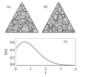
Figure 1: (a–b) Two different mechanically stable force configurations for a “snooker-triangle” packing of 210 balls; the thickness of the lines is proportional to the contact force. The “force network ensemble” samples all possible force configurations for a given contact network with an equal probability. (c) After sampling many force configurations, this yields the following distribution of interparticle forces $P(f)$.

Our ensemble approach is in the same spirit of the Edwards ensemble, in which an equal probability for all “blocked” or “jammed” configurations is postulated edwards ; kurchan . This Edwards ensemble does not only average over forces, but also over all possible packing configurations, which makes the problem difficult to track theoretically. We therefore propose to exploit the separation of length scales that occurs for hard particles, by fixing the packing geometry (macroscopic scale) and allowing for force fluctuations (microscopic scale). Besides practical advantages, the conceptual gain of separating the contact geometry from the forces is that we can start to disentangle the separate roles of contact and stress anisotropies PRL ; vanel ; 2Dbehringer . Interestingly, the idea to restrict the Edwards ensemble to fixed packing geometry has also been proposed recently by Bouchaud in the context of extremely weak tapping jp , and was also employed in recent simulations Unger ; herrmannensemble . Note that this force ensemble incorporates the local force balance equations on all particles and therefore it is fundamentally different from recent entropy-based models for force statistics ngan ; max_entropy . In these studies one postulates an entropy functional in terms of the single force distribution $P(f)$, without including the intricately coupled force balance equations and resulting force correlations.

From a more general point of view, the ensemble provides a challenging statistical physical problem of rather broad interest, that of sampling the solution space of a set of underdetermined equations and constraints. For example, the problem is mathematically very similar to the so-called flux balance analysis that is used to unravel metabolic networks in biological systems nature ; otherbio . Here the reaction fluxes are underdetermined and play a role analogous to the forces discussed here. In contrast to the forces, however, these fluxes typically display power-law distributions nature . This touches upon the deep question of what kind of statistics emerges when balancing scalars on a network of a given structure loadnetwork ; qmodel , and shows that the nature of the set of balance equations has a strong influence on the resulting statistics.

The aim of this paper is to explore the “phase space of force networks” and to unravel how this gives rise to the robust characteristics of the force distribution $P(f)$. We will initially focus on regular packings which are highly coordinated and therefore far from the isostatic limit. The advantage of these packings is, however, that the underlying physics is more transparent and that small regular packings can be resolved analytically. In addition, their force distributions are quite comparable to those found in numerical explorations of the ensemble for amorphous packings presented elsewhere PRL ; longnumerics . We will also study the ensemble on generalized networks, for which the force distributions rapidly loose their similarity to those of real packings.

After defining the ensemble in more detail, the paper consists of four parts. In Sec. II, we study the force ensemble for spherical, frictionless particles in regular triangular “snooker” packings. We discuss how these force distributions are related to geometric aspects of the high-dimensional phase space. In Sec. III we provide a formal mathematical description of the ensemble and derive the explicit form of $P(f)$, Eq. (7). This expression contains coefficients that depend on the packing geometry, and which we have been able to compute for several small systems. These exact $P(f)$ already exihibit the features that are relevant for larger, more realistic packings, and will be presented in Sec. IV. Due to the linearity of the equations of force balance, the problem can be further generalized by considering perturbations of the packing matrix and random matrices, which are presented in Sec. V. This probes which ingredients are essential for obtaining realistic $P(f)$’s. The paper closes with a discussion of the strengths and weaknesses of our approach and indicates some open issues and other problems that can be addressed with the ensemble.

I.1 Definition of the force network ensemble

We will now introduce the main aspects of the ensemble approach. Even though our approach is perfectly suited to include frictional forces PRL ; Unger ; herrmannensemble , for simplicity we will restrict ourselves to packings of $N$ frictionless spheres of radii $R_{i}$ with centers ${\bf r}_{i}$. We denote the interparticle force on particle $i$ due to its contact with particle $j$ by ${\bf f}_{ij}$. There are $zN/2$ contact forces in such packings ($z$ being the average contact number), and for purely repulsive central forces we can write ${\bf f}_{ij}=f_{ij}{\bf r}_{ij}/|{\bf r}_{ij}|$, where all $f_{ij}~{}(=f_{ji})$ are positive scalars. For a fixed contact topology in $d$ dimensions, we are thus left with $dN$ unknown positions ${\bf r}_{i}$ and $zN/2$ unknown forces $f_{ij}$. Note that the number of unknown forces is not precisely, but close to, $zN/2$ if boundary forces are present.

These degrees of freedom satisfy the conditions of mechanical equilibrium,

$$dN~{}\mbox{eqs.:}\hskip 8.53581pt\sum_{j}f_{ij}\,\frac{{\bf r}_{ij}}{|{\bf r}_{ij}|}={\bf 0},\hskip 14.22636pt\mbox{where }{\bf r}_{ij}={\bf r}_{i}-{\bf r}_{j},$$ (1)

and once a force law $F$ is given, the forces are explicit functions of the particle locations:

$$zN/2~{}\mbox{eqs.:}\hskip 14.22636ptf_{ij}=F({\bf r}_{ij};R_{i},R_{j})~{}.$$ (2)

The contact number $z$ is a crucial quantity. As has been argued before PRL ; isostatic ; isostatic2 , even though packings of infinitely hard frictionless particles have $z=2d$ and are thus isostatic, for particles of finite hardness, packings are typically hyperstatic with $z>2d$. In this paper we focus on hyperstatic packings, but before doing so, we wish to point out an important subtlety. In recent numerical work, it was shown that $z$ approaches the isostatic limit for vanishing pressures (hence vanishing deformations) of the particles, and that the (un)jamming transition here is similar to a phase transition, with power-law scaling of the relevant quantities and the occurrence of a large, possibly diverging lengthscale epitomy . Therefore, the precise value of $z$ may be important, since it reflects the distance to the jamming phase transition; this may bear on the interpretation of our results. It is worth pointing out that for frictional packings, even in the limit of infinitely hard particles, $z$ stays away from the isostatic limit grestcoord ; kasahara . Hyperstatic packings are therefore important, and our work, even though it focusses on frictionless packings, may also be seen in this light.

Returning to the force network ensemble, in the regime where particles are hard but not infinitely hard, variations of the force of order $\langle f\rangle$ result in minute variations of ${\bf r}_{ij}$. Hence, Eqs. (1) and (2) can effectively be considered separated, and the essential physics is then given by the force balance constraints Eqs. (1) with fixed ${\bf r}_{i}$. In this interpretation there are more degrees of freedom $(zN/2)$ than constraints $(2N)$, leading to an ensemble of force networks for a fixed contact geometry.

This ensemble for a fixed contact geometry is then constructed as follows. (i) Assume an a-priori flat measure in the force phase space $\{f\}$. (ii) Impose the $2N$ linear constraints given by the mechanical equilibrium Eqs. (1). (iii) Consider repulsive forces only, i.e., $\forall f_{ij}\geq 0$. (iv) Set an overall force scale by applying a fixed pressure or fixed boundary forces, similar to energy or particle number constraints in the usual thermodynamic ensembles.

We are thus considering the phase space defined by the force balance Eqs. (1), the condition that all $f$’s are positive, and a “pressure” constraint $\sum_{k}f_{k}=F_{\rm tot}$. For notational convience, we indicate the forces by a single index $k$ throughout the remainder of paper. Since all equations are linear, the problem can be formulated as

$${\cal A}\vec{f}=\vec{b}\quad\quad{\rm and}\quad\forall\quad f_{k}\geq 0~{},$$ (3)

where the fixed matrix ${\cal A}$ is determined by the packing geometry, $\vec{f}=(f_{1},f_{2},\cdots,f_{zN/2})$, and $\vec{b}=(0,0,0,\cdots,0,F_{\rm tot})$.

II Regular packings: balls in a snooker triangle

In the introduction we have seen that our ensemble approach for a snooker packing of 210 particles reproduces a force distribution that is very similar to those obtained in experiments and simulations. To understand how this shape of $P(f)$ comes about, we now work out the force network ensemble for small systems of crystalline (monodisperse) packings. We first study the packing of 3 balls shown in Fig. 2, for which we explicitly construct the phase space of force networks. As this system is very small, the force distribution deviates considerably from distributions observed in large systems. It nevertheless provides a very instructive example. We then present a numerical analysis of how $P(f)$ evolves as a function of system size for snooker packings. Remarkably, a packing of 6 balls is already sufficiently large to obtain the characteristic peak in $P(f)$. We therefore address general physical aspects by elaborating on this system.

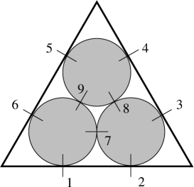
Figure 2: Three monodisperse frictionless spheres in a snooker triangle. This system has 9 unknown forces: 6 boundary forces ($f_{1}$ to $f_{6}$) and 3 interparticle forces ($f_{7}$, $f_{8}$, $f_{9}$).

II.1 Three balls

In the system of 3 balls depicted in Fig. 2, we encounter 9 unknown forces: 6 boundary forces and 3 interparticle forces. These forces have to balance on each particle in both the $x$ and $y$ directions, which constitute $2\times 3=6$ linear constraints. In addition, we impose an overall pressure by keeping the total force on a boundary at a fixed value: for example we fix $f_{1}+f_{2}=2$. Interestingly, one can show that such a boundary or pressure constraint is equivalent to keeping the sum over all forces at a fixed value: in appendix A we demonstrate that keeping $\sum_{j}f_{j}$ at a constant value is equivalent to a constant pressure, also for irregular packings.

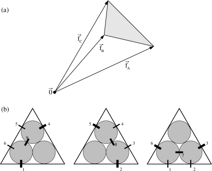
Figure 3: (a) The 2D phase space of the 3-ball problem can be defined using three simple independent solutions of the problem. (b) The first solution $\vec{f}_{A}$ has $f_{1}=f_{4}=2$, $f_{5}=f_{6}=1$ and $f_{9}=\sqrt{3}$ and $f_{2,3,7,8}=0$; the other solutions $\vec{f}_{B}$ and $\vec{f}_{C}$ follow from the threefold symmetry of the packing.

Together with the pressure constraint, there are thus 7 linear equations to determine the 9 unknown forces $\vec{f}=(f_{1};,\cdots,f_{9})$, and hence, there is a two-dimensional space of solutions. This space does not contain the origin of the force space, for which all $f_{j}=0$, due to the inhomogeneous pressure constraint. As a consequence one requires three vectors to characterize the two-dimensional space: two basis vectors and a vector defining the location of the plane with respect to the origin. Using linear algebra one can construct these three vectors from three linearly independent force network solutions $\vec{f}_{A}$, $\vec{f}_{B}$, $\vec{f}_{C}$, which allows to express the general solution as

$$\vec{f}=c_{A}\vec{f}_{A}+c_{B}\vec{f}_{B}+(1-c_{A}-c_{B})\vec{f}_{C}~{}.$$ (4)

An intuitive picture of this equation is provided in Fig. 3a: the 2-dimensional plane can be defined from three solutions (very much like a line can be defined by two points). However, the constraints that all $f_{j}\geq 0$, provide serious limitations on the allowed values of $c_{A}$ and $c_{B}$. As will be shown below, only a small convex subset of the the two-dimensional solution space represents force networks consisting of strickly repulsive forces.

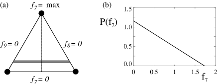
Figure 4: Two dimensional cut through the phase-space spanned by the nine forces of the 3-ball problem. (a) The borders of the triangle are the lines where one of the interparticle forces changes sign; the shaded area represents the probability to find a configuration between $f_{7}$ and $f_{7}+\delta f_{7}$. (b) The corresponding force distribution $P(f_{7})$.

Using the solutions of Fig. 3 to construct the phase space, we obtain the triangle depicted in Fig. 4a. In this picture, the three solutions are the corners of the triangle. For example, the right corner represents the first solution in Fig. 3, $\vec{f}_{A}$ for which $(f_{7},f_{8},f_{9})=(0,0,\sqrt{3})$, whereas the left corner corresponds to $\vec{f}_{B}$ that has $(f_{7},f_{8},f_{9})=(0,\sqrt{3},0)$. A superposition of these two vectors is still a solution of our linear problem, and since in both cases $f_{7}=0$, the base of the triangle is a line where $f_{7}=0$. The upper corner represents $\vec{f}_{C}$, for which $f_{7}$ attains its maximum value of $\sqrt{3}$. Therefore, the dashed line is a projection of the $f_{7}$ axis onto this 2D space of solutions. This implies that the space below the triangle corresponds to a region where $f_{7}<0$, which is forbidden for repulsive particles. Applying the same argument for $f_{8}$ and $f_{9}$, one realizes that only the area inside the triangle is allowed. As we mentioned in the introduction, the ensemble assumes an equal a priori force probability, which makes each point in the triangle equally likely (due to the linearity of the force balance restrictions). Therefore, the probability to have a solution between $f_{7}$ and $f_{7}+\delta f_{7}$ is simply represented by the shaded area in Fig. 4a. This “volume” decreases linearly as $f_{7}$ approaches its maximum value, so that the distribution of $f_{7}$ simply becomes $P(f_{7})=\frac{2}{3}(\sqrt{3}-f_{7})\Theta(\sqrt{3}-f_{7})$ – see Fig. 4b.

The combination $x\Theta(x)$, where $\Theta(x)$ is the Heaviside step function, will occur in most $P(f)$ thoughout this paper. Therefore we introduce

$$\mathcal{T}(x)\equiv x\Theta(x)~{}.$$ (5)

Figure 5: Two dimensional cut through the phase-space spanned by the nine forces of the 3-ball problem, showing how boundary forces are distributed. (a) The borders of the hexagon are the lines where one of the boundary forces changes sign; the shaded areas represents the probability for a certain $f_{1}$. (b) The corresponding force distribution $P(f_{1})$.

The distribution of the boundary forces ($f_{1}$ to $f_{6}$) can be found in a similar manner. Checking the three independent solutions, one finds that $f_{1}=0$ at the left corner, $f_{1}=1$ at the upper corner, and $f_{1}=2$ at the right corner of the “phase space triangle”. From the geometric construction in Fig. 5a, it is easy to find the $f_{1}=0$ line, and the projection of the $f_{1}$ axis is indicated by the arrow. Due to symmetry there are of course six such borders ($f_{1}=0$ to $f_{6}=0$), and all boundary forces are positive inside the hexagon. So, the solutions for which all forces are positive lie within the triangle. Considering the shaded area in Fig. 5a, we obtain the distribution of boundary forces $P(f_{1})=\mathcal{T}(2-f_{1})-2\mathcal{T}(1-f_{1})$, which is shown in Fig. 5b. We thus find that there is a qualitative difference between the boundary forces $(f_{1},\cdots,f_{6})$ and the interparticle forces $(f_{7},f_{8},f_{9})$. Interestingly this is also the case for larger systems and is consistent with earlier work on statistics of wall forces rapid ; loooong .

Although this 3-ball system provides a very nice illustration of how to obtain $P(f)$ from all possible force configurations, it is not complex enough to reproduce non-monotonic $P(f)$. In fact, the problem discussed above is equivalent to partitioning a conserved energy into 3 positive parts. In our case, the conserved quantity is the total force and the 3 parts are the coefficients $c_{A}$, $c_{B}$ and $(1-c_{A}-c_{B})$. In the thermodynamic limit, the problem of partitioning, e.g., an energy $E_{\rm tot}$ simply yields the Boltzmann distribution of energies $E_{i}$ of subsystems; also for finite systems these distributions are always monotonically decreasing – see appendix A. In Sec. II.3, we show that the problem of 6 balls already has enough complexity that it leads to non-monotonic behavior of $P(f)$.

II.2 Numerical analysis of larger systems

Figure 6: $P(f)$ for bulk forces in “snooker” packings of increasing sizes.

To compute $P(f)$ for larger packings, we have applied a simulated annealing procedure numrec . As was shown in our previous work PRL this scheme can also be used for irregular packings. Starting from an ensemble of random initial force configurations taken from an arbitrary distribution with $\langle f\rangle=1$ and $f_{j}\geq 0$, we select a random bond $j$ and add a random force $\Delta f$, so that $f_{j}(n)=f_{j}(o)+\Delta f$, in which the symbols $n$ and $o$ denote the new and old force respectively. The random change from $o$ to $n$ is accepted with a probability given by the conventional Metropolis rule $p(o\rightarrow n)=\min\left(1,\theta\left(f_{j}(n)\right)\exp\left[-\left({\cal H}(n)-{\cal H}(o)\right)/T\right]\right)$, in which $\cal{H}$ is a penalty function whose degenerate ground states are solutions of Eq. (3):

$${\cal H}(\vec{f})=\left({\cal A}\vec{f}-\vec{b}\right)^{2}.$$ (6)

For large packings ($N>500$) it is computationally much more efficient to always satisfy $\langle f\rangle=1$ by selecting two bonds ($j\neq k$) at random and using $f_{j}(n)=f_{j}(o)+\Delta f$ and $f_{k}(n)=f_{k}(o)-\Delta f$ as the update scheme, so that the pressure constraint can be left out of the penalty function. By slowly taking the limit of $T\rightarrow 0$ we sample all mechanically stable force configurations for which ${\cal H}\rightarrow 0$. We have carefully checked that results do not depend on the initial configurations and details of the annealing scheme. In section IV we will show that this scheme perfectly reproduces analytic results for small regular packings.

The two force networks shown in Fig. 1 are typical solutions $\vec{f}$ obtained by this procedure. The resulting distributions of interparticle forces are presented in Fig. 6, for packings of increasing number of balls; boundary forces will be discussed seperately and are not included in these $P(f)$. Note that all $P(f)$’s display a peak for small $f$, which is typical for jammed systems liuletter . The fact that the probability for vanishing interparicle forces remains finite is in agreement with most numerical and experimental observations; only a few studies report power-law behavior for small forces radjai96 ; lovol . For large packings, this peak rapidly converges to its asymptotic limit. The tail of $P(f)$ broadens with system size, and will be discussed in more detail in Sec. VI.

Figure 7: Boundary forces for “snooker” packings of increasing sizes.

In Fig. 7 we show the probability distributions $P(f_{\mathrm{wall}})$ for the forces $f_{\mathrm{wall}}$ between sidewalls and balls for the regular packings of increasing size. As has been discussed at length in rapid ; loooong , these distributions differ from the probability distributions of bulk forces. In this particular case this is easy to see: the boundary force $f_{\mathrm{wall}}$ has to balance the force of the two balls in the next layer with which it makes contact (excluding the corner balls). Even though each of these forces has a finite probability to be vanishingly small, the probability that both these forces are small has not, hence $P(f_{\mathrm{wall}})\rightarrow 0$ for $f_{\mathrm{wall}}\rightarrow 0$.

II.3 $P(f)$ and phase space geometry

Here we will discuss some geometrical aspects of the set of allowed force configurations. Consider the $zN/2$ dimensional force phase space spanned by the ${f_{j}}$. Since all $2N$ force balance equations (1) are linear in the forces, the allowed solutions lie on a hyperplane of dimension $(zN/2-2N)$. (Note that the overall pressure constraint introduces an additional constraint, lowering the dimension by 1.) Furthermore, since we consider repulsive forces only, this plane is restricted to the “positive” hyperquadrant where all $f_{j}\geq 0$ (see Fig. 8). Therefore, the allowed force-configurations form a (hyper)-polygon whose facets are given by the conditions that some force $f_{j}$ becomes 0. Under our assumption of a “flat measure”, all points on this polygon correspond to valid force networks with equal probability.

A number of basic properties of this solution space can now readily be deduced. Trivially, the solution space is convex: due to the linearity of the equations, the points on a straight line connecting two admissible solutions are admissible solutions themselves, as was also pointed out in bioconvex ; Unger ; herrmannensemble . Although this is not immediately obvious in low dimensions, for higher dimensional bodies the overwhelming part of the “measure” is concentrated near the boundary (think of a high dimensional sphere, where almost all volume is in the “shell” close to surface). Near the boundaries, one or more forces tend to zero, and this is consistent with the fact that in typical force networks a finite fraction of the forces are close to zero (since $P(f\downarrow 0)\neq 0$). More homogeneous force networks, for which all forces are around some average value, correspond to points in the phase space that are sufficiently far away from the boundary. While such configurations are perfectly allowed within our framework, and are easy to construct by considering a suitable linear combination of “ordinary” force-networks, they only occur with vanishingly small probability in the limit of large $N$, and are thus extremely unlikely to be seen in “unguided numerics” or experiments.

Even though we have not worked this out in detail, we expect that some more general properties of the force networks could be related to geometrical properties of (random) hyperpolygons. As one simple example consider the following. For two forces, say $f_{i}$ and $f_{j}$, to become zero simultaneously, the facets $i$ and $j$ have to touch; in general this may not be possible geometrically, so that an intruiging issue concerning correlations between distant forces arises.

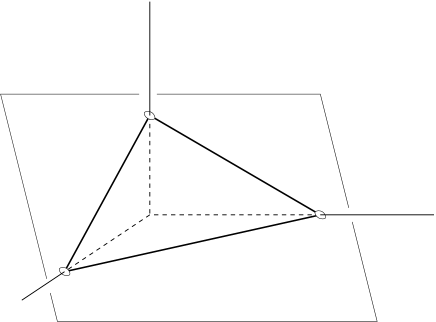
Figure 8: Schematic representation of the phase space of allowed force configurations. Each $f_{ij}$ defines a direction in the $zN/2$ dimensional force space. By imposing the linear conditions of mechanical equilibrium, this space is restricted to a “hyperplane” of lower dimensionality. The physically allowed region is a (hyper)polygon is bounded by the requirement that all $f_{ij}\geq 0$.

Another issue that may have a relatively simple interpretation in the polygon language is the peaked appearance of $P(f)$. We suggest the following intuitive picture, based on a consideration why the slope $dP(f)/df$ can be expected to be positive for small forces. For very small systems, like the case of 3 balls discussed in section II.1, this is not true. This immediately follows from the shape of the allowed phase space polygon. As shown in Fig. 4, this is a triangle where the angles between the bounding edges were acute. When we move away from a $f=0$ boundary, the phase space volume decreases so that $dP/df<0$. If we go to larger systems, however, the number of facets bounding the space $(=zN/2)$ becomes much larger than the dimension $D$ $(=zN/2-dN-1)$ of the polygon. Hence, we expect that the “angles” between bounding facets will typically become obtuse, which will make the phase space increase when increasing $f$. This indicates that $dP/df$ is typically positive for small forces, so that $P(f)$ displays a peak footfacets .

Six balls – Let us provide another perspective on the phase space geometry by discussing the problem of 6 balls, which is the smallest snooker packing displaying a non-monotonic $P(f)$. For the 6 balls there are $18$ forces, which are constrained by $2\times 6+1=13$ equations, so the space of solutions is a 5D hyperplane. If we try to construct the phase space like we did for the 3 balls, we now require 6 independent solutions $\vec{f}$ that obey force balance on each particle. Again, there exist simple solutions of linearly propagating force lines - see Fig. 9a. However, there are only 3 such solutions, so we also require nontrivial solutions where forces “scatter” at a certain particle. For example, we can take 3 solutions of the type shown in Fig. 9b.

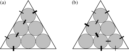
Figure 9: Two different types of solutions of force equilibrium for 6 balls in a snooker-triangle.

The presence of these nontrivial solutions changes the phase space in a a fundamental manner. A given force can now take a certain value in many different ways, by different linear combinations of elementary “modes”. In other words, a force can no longer be associated to a single mode of the force network, like it was the case for the three interparticle forces in Fig. 3. As a consequence, the problem has become much more intricate than simply partitioning the total force into positive amplitudes (which, for large systems, would lead to a simple exponential distribution, see appendix A). Instead one finds nontrivial force distributions, for which we derive analytical expressions in the following section. Indeed, for all investigated packings, we observe non-monotonic $P(f)$ whenever scatter-solutions occur.

III General formulation for arbitrary packing geometry

In this section we show how statistical averages can be computed analytically within the force network ensemble, for arbitrary packings. We present a systematic way to evaluate the complicated high-dimensional integrals as a sum over contributions of the following structure:

$$P(f) = \sum_{\lambda}c_{\lambda}\,f^{q_{\lambda}}(1-b_{\lambda}f)^{D-1-q_{\lambda}}\Theta(1-b_{\lambda}f)$$ (7)

$$= \sum_{\lambda}c_{\lambda}\,f^{q_{\lambda}}\left[\mathcal{T}(1-b_{\lambda}f)\right]^{D-1-q_{\lambda}}~{},$$

where $D$ is the dimension of the phase space, and the coefficients $b_{\lambda}$, $c_{\lambda}$ and $q_{\lambda}$ depend in a nontrivial way on the particle packing; for most $\lambda$, we find that $q_{\lambda}=0$. The function $\mathcal{T}$ was defined in Eq. (5); note that the contributions $\left[\mathcal{T}(1-bf)\right]^{D-1}\sim e^{-(D-1)bf}$ in the thermodynamic limit. For the reader who is interested in the results but not in the details of the derivation, we summarize exact $P(f)$ for small regular packings in Sec. IV.

III.1 Mathematical definition of the ensemble

The phase space of force networks is defined by the linear constraints of force balance, an inhomogeneous linear constraint to fix the pressure, and the requirement that all forces are non-negative. If we now indicate each contact force by an index $j$, we can express mechanical equilibrium as

$$\sum_{j=1}^{zN/2}a_{ij}f_{j}=0~{},$$ (8)

where the nonzero $a_{ij}$ are projection factors between $-1$ and $+1$. There are $dN$ such equations, which we label as $i=2,3,\cdots,dN+1$. To keep the overall pressure at a fixed value we impose $\sum_{j}f_{j}=F$, which for notational convience we write as

$$\sum_{j=1}^{zN/2}a_{1j}f_{j}=F~{},\quad\quad\mbox{\rm with all}\quad a_{1j}=1~{}.$$ (9)

We thus encounter a matrix problem ${\cal A}\vec{f}=\vec{b}$, where the $a_{ij}$ are the components of ${\cal A}$.

Imposing the various constraints and assuming an equal a priori probability in the force space defined by $\vec{f}=(f_{1},f_{2},\cdots,f_{zN/2})$, we obtain the joint probability density

$$P(\vec{f}) = \frac{1}{\Omega}\,\delta\left(\sum_{j}a_{1j}f_{j}-F\right)\prod_{i\geq 2}\delta\left(\sum_{j}a_{ij}f_{j}\right)~{},$$ (10)

which is normalized by the phase space volume

$$\Omega=\int d\vec{f}\,\delta\left(\sum_{j}a_{1j}f_{j}-F\right)\prod_{i\geq 2}\delta\left(\sum_{j}a_{ij}f_{j}\right)~{}.$$ (11)

Since we consider repulsive forces, $\int d\vec{f}$ represents an integral over all forces in the hyperquadrant where all $f_{j}\geq 0$. With this measure, we can now compute the single force distribution $P(f_{j})$ as

$$P(f_{j})=\left[\prod_{k\neq j}\int_{0}^{\infty}df_{k}\right]\,P(\vec{f})\,~{},$$ (12)

which in principle can be different for each $f_{j}$; for example see the boundary forces within the snooker-triangles (Sec. II). In practice, it turns out that $P(f_{j})$ for different interparticle forces shows only little variation.

The fact that we only integrate over the hyperquadrant where all $f_{j}\geq 0$ makes it difficult to evaluate the integrals explicitly: each integration of the $\delta$ function gives rise to a Heaviside $\Theta$ function to keep track of the boundaries of the phase space. To avoid this problem we represent the $\delta$ functions as Fourier integrals

$$\delta\left(\sum_{j}a_{ij}f_{j}\right)=\int_{-\infty}^{\infty}\frac{ds_{i}}{2\pi}\,e^{-is_{i}\sum_{j}a_{ij}f_{j}}~{},$$ (13)

which has the advantage that the $f_{j}$ only occur in an exponential way and they are easily integrated out. If we now write $\vec{s}=\frac{1}{2\pi}(s_{1},\cdots,s_{m})$, where $m=dN+1$, the partition function $\Omega$ becomes

$$\Omega = \int_{-\infty}^{\infty}d\vec{s}\,e^{is_{1}F}\,\prod_{j}\int_{0}^{\infty}df_{j}\,e^{-(\epsilon_{j}+i\sum_{i}s_{i}a_{ij})f_{j}}$$ (14)

$$= \int_{-\infty}^{\infty}d\vec{s}\,e^{is_{1}F}\,\prod_{j}\frac{1}{i(-i\epsilon_{j}+\sum_{i}s_{i}a_{ij})}~{},$$

where the factor $e^{is_{1}F}$ arises due to the inhomogeneous pressure constraint (9). We furthermore added cut-off factors $e^{-\epsilon_{j}}$ so that the integrations over the $f_{j}$ are definite; at the final stage we take the limit $\epsilon_{j}\rightarrow 0$. The rows of the matrix ${\cal A}$ correspond to the constraint variables $s_{i}$ and the columns correspond to the denominators originating from the $f_{j}$ integrals. From now on we indicate the dimensions of the matrix by $m=dN+1$ (number of rows) and $n=zN/2$ (number of columns).

All integration variables $s_{i}$ run from $-\infty$ to $\infty$, so we can evaluate them as contour integrations in the complex plane. The integrand is a product of denominators, and each $s_{i}$ occurs in as many denominators as there are forces acting on a certain particle. In the absence of gravity, each mechanically stable particle should at least have $3$ contacts. This makes the integration over the $s_{i}$ converging at infinity and allows to close the contour either through the upper half plane or through the lower half plane. An exception is the $s_{1}$ integration, which has to be closed through the upper plane since $F>0$.

Let us first integrate out $s_{m}$. Each denominator that has $a_{mj}\neq 0$ gives rise to a pole at

$$s_{m}(j)=\frac{1}{a_{mj}}\left(i\epsilon_{j}-\sum_{i=1}^{m-1}s_{i}a_{ij}\right)~{}.$$ (15)

The residue is obtained by substiting this pole in the remaining $n-1$ denominators of Eq. (14). Note the importance of the $\epsilon_{j}$ to make the integration definite. It is easily seen that this substitution leads to a renormalized matrix ${\cal A}^{*}$ of $m-1$ rows (constraint variables) and $n-1$ columns (denominators), and to renormalized $\epsilon_{j^{\prime}\neq j}^{*}$ as well. However, the key observation is that the remaining integrals are of the same type as Eq. (14). We thus find a recursion relation

$$\Omega_{mn}({\cal A})=\pm\sum_{j}\frac{1}{a_{mj}}\,\Omega_{m-1,n-1}({\cal A}^{*}_{j})~{},$$ (16)

where the sum extends over all encircled poles. The symbol $\pm$ indicates that the contribution is positive or negative depending on whether the integral has been closed through the upper ($+$) or lower ($-$) half plane. The renormalization to ${\cal A}^{*}_{j}$ is different for each pole, so each term has to be followed independently. At each integration the number of contributions therefore grows rapidly, since each new pole gives rise to a new “branch” of the recursion Eq. (16). The exponential increase of the number of branches with the size of the tree forms a severe limitation on the solutions for larger systems. At the final stage, we have to compute $\Omega_{1,n_{\rm final}}=\Omega_{1,D+1}$ by integrating over $s_{1}$:

$$\Omega_{1,D+1} = \int_{-\infty}^{\infty}\frac{ds_{1}}{2\pi}\,e^{is_{1}F}\,\prod_{j}\frac{1}{i(-i\epsilon_{j}+s_{1}a_{1j})}$$ (17)

$$= \frac{F^{D}}{D!\prod_{j}a_{1j}}~{},$$

where $D$ is the dimensionality of the phase space. The $a_{1j}$ and ${\epsilon_{j}}$ appearing in this equation are obtained from successive renormalization each time a pole is substituted.

So, the calculation of $\Omega$ involves a tree-like structure where the branching rate is equal to the number of encircled poles. Using relation Eqs. (16) and (17) one can compute the contribution of each individual branch, using a recursive scheme. The fact that $\Omega$ scales as $F$ to the power $D$ is not surprising: $F$ is the only force scale for the $D$ dimensional phase space, and in fact, the behavior $F^{D}$ is obtained immediately from a trivial rescaling of Eq. (11). However, in the following paragraphs we show how the analysis presented above can be extended to the nontrivial calculation of the force distribution $P(f)$.

III.2 Calculation of $P(f)$

Comparing Eqs. (11) and (12), we notice that the expression for $P(f_{j})$ is the same as that for $\Omega$ without the integration over $f_{j}$; without loss of generality we will consider $P(f_{1})$. As a result, the expression for $P(f_{1})$ contains one less dominator than Eq. (14) and instead there will be an additional exponential factor, i.e.

$$P(f_{1}) = \frac{1}{\Omega}\int d\vec{s}\,e^{i\left(s_{1}F-f_{1}\sum_{i}s_{i}a_{i1}\right)}\,e^{-\epsilon_{1}f_{1}}$$ (18)

$$\times\,\prod_{j\neq 1}\frac{1}{i(-i\epsilon_{j}+\sum_{i}s_{i}a_{ij})}~{}.$$

Following the same integration strategy as for $\Omega$, we again obtain a recursion of the type

$$P_{m,n}(f_{1})=\pm\sum_{k}\frac{1}{a_{mk}}\,P_{m-1,n-1}(f_{1})~{},$$ (19)

where for clarity in notation we left out the explicit dependence on the (renormalized) matrix ${\cal A}$. After successive substitution of the poles, the final integration over $s_{1}$ becomes

$$P_{1,D+1}(f_{1}) = \frac{1}{\Omega}\int_{-\infty}^{\infty}\frac{ds_{1}}{2\pi}\,e^{is_{1}\left(F-a_{11}f_{1}\right)}\,e^{-\epsilon_{1}f_{1}}$$

$$\times\,\prod_{j\neq 1}\frac{1}{i(-i\epsilon_{j}+s_{1}a_{1j})}$$

$$= \frac{1}{\Omega}\,\frac{\left(F-a_{11}f_{1}\right)^{D-1}}{(D-1)!\prod_{j\neq 1}a_{1j}}\,\Theta\left(F-a_{11}f_{1}\right)~{}.$$

Each branch of the tree gives a contribution of this type and together they accumulate to the result of Eq. (7) with $q_{\lambda}=0$. The coefficients $b_{\lambda}$ are thus simply the $a_{11}/F$ that remain after successive renormalization of the matrix ${\cal A}$. We will demonstrate that, fortunately, the final result contains only a few different $b_{\lambda}$, at least for small packing geometries.

In the final integration of Eq. (III.2), we implicitly assumed that all $a_{1j}$ appearing in the denominators are not equal to zero. They may become negative, provided that the associated small $\epsilon_{j}$ is also negative so that the pole is still in the upper half plane and the integration remains finite. Naively one would expect that it very unlikely that some $a_{1j}=0$, since it corresponds to an accidental coincidence of two poles. However, for regular structures like the snooker-packings it is a frequently occuring phenomenon. The double poles are responsible for the cases $q_{\lambda}\neq 0$. We have adapted the algorithm such that it can deal with an arbitrary multiplicity of the poles. In some cases, these multiple poles alter the general result for $P(f)$ with additional contributions of the type

$$P_{\lambda}(f)\propto f^{q_{\lambda}}\left(1-b_{\lambda}f\right)^{D-1-q_{\lambda}}\,\Theta\left(1-b_{\lambda}f\right)~{}.$$ (21)

These contributions can be recognized as the $q_{\lambda}$th derivatives of the general result, corresponding to the coincidence of $q_{\lambda}+1$ poles. We expect, however, that multiple poles will never occur for disordered packings.

IV Exact results for small crystalline packings

We now present a number of exact $P(f)$ for small crystalline packing geometries. In particular, we have worked out the problem of 6 balls in a snooker-triangle, triangular 2D packings with periodic boundary conditions, as well as a small 3D FCC packing with periodic boundary conditions. Following the algorithm described in the previous section, we have been able to obtain the coefficients $b_{\lambda}$ and $c_{\lambda}$ appearing in Eq. (7) for these systems. For notational convenience, we express the results in the dimensionless force $x=f/F$. All is in perfect agreement with our numerical simulations.

The intricate combinatorics has been performed using a computer program. As mentioned the number of contributions grows exponentially with the size of the tree, since the branching rate is of order of 2 per elimination step. Even worse is the fact that the different signs of the contributions lead to large cancellations. The results given below for small systems are the result of many more terms in the tree. This makes the algorithm numerically unstable for larger systems.

IV.1 2D triangular packings with periodic boundaries

Four balls – The smallest interesting 2D triangular packing with periodic boundary conditions is the $2\times 2$ packing of 4 balls. It has $3\times 4=12$ unknown forces and $2\times 4=8$ equations expressing mechanical equilibrium. Due to the periodic boundaries, however, two of these equations are actually dependent. Hence there are only $6$ independent equations and together with the overall pressure constraint this results into a $D=12-(6+1)=5$ dimensional phase space.

In terms of the dimensionless variable $x=f/F$, we obtained the following result for this system:

$$P(x)=10\,\mathcal{T}^{4}(1-2x)~{}.$$ (22)

Taking $F=12$ so that $\langle f\rangle=1$, we plotted this distribution in Fig. 10b. It is a monotonically decreasing function that allows a maximum force of $x_{\rm max}=\frac{1}{2}$,i.e., $f_{\rm max}=\frac{1}{2}F$. This maximum force is achieved for a simple “propagating” solution shown in Fig. 10a: the total force $F$ is shared between two nonzero forces only (note the similarity to the solutions shown in Fig. 3 for the packing of three balls). Due to the symmetry of the problem there are six such trivial solutions, which are in fact sufficient to define the whole 5D phase space of force networks. The $2\times 2$ problem is therefore equivalent to partitioning the total force into six nonnegative “amplitudes”, just as was the case for the three balls in the snooker-triangle. Indeed, Eq. (22) is of the same form as Eq. (36) in appendix A.

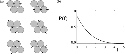
Figure 10: (a) All solutions of the $2\times 2$ periodic arrangement can be described as a superposition of linearly propagating force-lines. (b) The corresponding monotonic $P(f)$.

Figure 11: (a) The system of $3\times 3$ balls allows for nontrivial “scatter” solutions. (b) The corresponding $P(f)$ is therefore non-monotonic. The solid curve is Eq. 23; the crosses are obtained from numerics as described in section II.2.

Nine balls – For the $3\times 3$ packing of 9 balls there are $3\times 9=27$ unknown forces that are constrained by $2\times 9-2=16$ independent equations of mechanical equilibrium. Fixing the overall pressure, one is left with a $D=27-(16+1)=10$ dimensional phase space. This space can not be reconstructed from the trivial propagating solutions, of which there are only 9. Again, the presence of the “scatter” solutions such as the one shown in Fig. 11a results into a non-monotonic $P(x)$:

$$P(x)=40\left[\mathcal{T}^{9}(1-3x)-\frac{3}{4}\mathcal{T}^{9}(1-9x)\right]~{}.$$ (23)

Taking $F=27$ so that $\langle f\rangle=1$, we plotted $P(f)$ as a solid curve in Fig. 11b; the crosses indicate the distribution obtained by the same numerical method that was used for the snooker-triangles in Sec. II. The perfect agreement illustrates the accuracy of our numerical method.

IV.2 3D FCC packing with periodic boundaries

To illustrate that our ensemble can be applied to three dimensional packings just as well, we have computed $P(f)$ in the conventional FCC unit cell, with periodic boundary conditions. This is a system of 4 balls, since the FCC unit cell contains $8$ particles at corners (each counting for $1/8$) and $6$ particles at the faces (counting for $1/2$). The coordination number of the FCC packing is $z=12$, so there are $zN/2=24$ forces in this system. We now have to respect force balance in three dimensions, i.e. $3\times 4=12$ equations, of which, due to periodic boundary conditions, only $9$ turn out to be independent. Together with the pressure constraint, there are thus $10$ equations to constrain $24$ forces, and hence the problem has a $14$ dimensional space of solutions.

The resulting $P(x)$ turns out to be

$$P(x) = \frac{364}{9}\left[\mathcal{T}^{13}(1-2x)-\frac{9}{26}\mathcal{T}^{13}(1-6x)\right.$$ (24)

$$\left.-\frac{4}{13}\mathcal{T}^{13}(1-8x)-27x\mathcal{T}^{12}(1-6x)\right]~{}.$$

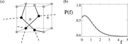
Figure 12: (a) One of the “scatter” solutions for the FCC unit cell with periodic boundary conditions. The black spheres belong to this unit cell; the grey spheres belong to neighbouring cells. All forces have the same magnitude; those within this unit cell are drawn as thick solid lines; the others are drawn as thick dashed lines. (b) The corresponding non-monotonic $P(f)$, from Eq. 24 (solid curve) and from numerics as described in section II.2 (crosses).

Fig. 12 shows that this force distribution has the same typical features as those obtained for two-dimensional packings. It’s a non-monotonic function, which can again be related to the existence of “scatter” solutions. There are 15 independent solutions to fix the 14D phase space of force networks, 12 of which are linearly propagating “trivial” solutions (two for each lattice direction). The other three are again “scatter” solutions. One of these is shown in Fig. 12.

IV.3 6 balls in a snooker-triangle

We now provide the exact force distributions for the 6 balls in a snooker-triangle, which we discussed in Sec. II. We already showed that one has to distinguish between the interparticle forces and the particle-wall forces, which obey qualitatively different statistics. Upon closer inspection, however, one notices that there are also two different types of interparticle force: the 6 closest to the boundary (type $I$) and the 3 closest to the center (type $II$). We find that

$$P_{I}(x)=\frac{95a^{5}}{768\left(7+4\sqrt{3}\right)}\times$$

$$\left[\mathcal{T}^{4}(1-ax)-\frac{16}{19}\mathcal{T}^{4}(1-2ax)+\frac{3}{19}\mathcal{T}^{4}(1-3ax)\right]~{},$$ (25)

$$P_{II}(x)=\frac{15a^{5}}{64\left(7+4\sqrt{3}\right)}\times$$

$$\left[\mathcal{T}^{4}(1-ax)-\frac{5}{6}\mathcal{T}^{4}\left(1-\frac{3}{2}ax\right)-ax\mathcal{T}^{3}\left(1-\frac{3}{2}ax\right)\right]~{}.$$ (26)

where $a=2\left(1+\sqrt{3}\right)$.

The numerical results shown in Fig. 6 were obtained without discriminating between type $I$ and type $II$. This is allowed since even though $P_{I}(x)$ and $P_{II}(x)$ are not identical, their shapes are very similar. Comparing the data with $\frac{2}{3}P_{I}(x)+\frac{1}{3}P_{II}(x)$ gives again an excellent agreement between the theoretical result and the numerical result shown in Fig. 6. The factors 2/3 and 1/3 appear because there are 6 forces of type $I$ and 3 forces of type $II$.

Finally, let us discuss the statistics for the boundary forces as shown in Fig. 7. Also in this case there are two different types of boundary forces, namely 6 at the corners $(c)$ and 3 in the middle $(m)$ of each boundary. We find that

$$P_{c}(x) = \frac{5b^{5}}{9\left(7+4\sqrt{3}\right)}\left[\mathcal{T}^{4}(1-bx)-\mathcal{T}^{4}(1-2bx)\right.$$

$$\left.-\frac{10}{3}bx\mathcal{T}^{3}(1-2bx)-2(bx)^{2}\mathcal{T}^{2}(1-2bx)\right]~{},$$

$$P_{m}(x)=\frac{5b^{5}}{54\left(7+4\sqrt{3}\right)}\times$$

$$\left[-\mathcal{T}^{4}(1-bx)+8bx\mathcal{T}^{3}(1-bx)+\mathcal{T}^{4}(1-2bx)\right]~{},$$ (28)

where $b=3+\sqrt{3}$. The linear combination $\frac{2}{3}P_{c}(x)+\frac{1}{3}P_{m}(x)$ fits the boundary force distributions as shown in Fig. 7 extremely well (not shown).

V Beyond Packings

In the preceding sections we have extensively studied the force distributions emerging in the ensemble of force networks, for a variety of crystalline packings. The various $P(f)$ are non-monotonic and display only marginal differences. As we demonstrated in Ref. PRL , the same qualitative behavior is observed for irregular packings. Even though the packing matrices differ substantially in these cases, the resulting $P(f)$ is extremely robust. This raises the question of which are the essential ingredients to obtain a typical force distribution. In other words, what properties of the packing matrix ${\cal A}$ determine the shape of $P(f)$?

All packing matrices consist of a large number of zeros, except for a few elements per row that are projection factors between $-1$ and $1$. Such a matrix has some features of a random matrix, but it implicitly contains the entire spatial structure of the system. To see whether this spatial structure is crucial for the typical shape of $P(f)$, we now study true random matrices, which no longer represent a physical packing of particles. Of course, we still extend the matrix by the normalization constraint $\sum_{j}f_{j}=F$ and demand that all $f_{j}\geq 0$.

We find that such random matrices yield $P(f)$ whose decay is described by a product of Gaussian and exponential tails. However, all these distributions are monotonically decreasing and thus lack the typical peak, even when considering “sparse” random matrices. We then try the opposite approach, where we start from a physical packing matrix and then slowly introduce randomness. In contrast to the striking robustness of $P(f)$ for real packings, the force distribution is very sensitive even to small perturbations away from the physical matrix.

V.1 Random matrices

V.1.1 Infinite Gaussian random matrices

We start out the random matrix approach by generating all elements $a_{ij}$ in Eq. (8) from a Gaussian distribution

$$P_{a}(a_{ij})=\sqrt{\frac{1}{\pi}}\,e^{-a_{ij}^{2}}~{},$$ (29)

for which the problem can be solved exactly. Together with the constraint $\sum_{j}f_{j}=F$, we obtain a matrix of $m$ rows and $n$ columns. By demanding that all $f_{j}\geq 0$, one can in principle follow the same analysis as for real packings; we then average over all possible random matrices and consider only solutions with all $f_{j}\geq 0$. In appendix B we derive that, in the limit that $n,m\rightarrow\infty$ with a fixed ratio $\rho=m/n$, the distribution becomes

$$P(f)=c(\rho)\,e^{-(1-\rho)f}\,e^{-b(\rho)f^{2}}~{},$$ (30)

where $b(\rho)$ is an almost linear function that has $b(0)=0$ and $b(1)=1/\pi$. For square matrices, i.e. $\rho=1$, we thus find that $P(f)$ is a pure Gaussian centered around $f=0$. This is illustrated in Fig. 13a; to calculate the $P(f)$ for these non-square matrices we have evaluated Eqs. (40) and (B) by Monte Carlo simulation. Tuning $\rho$ to zero, the pressure constraint is dominant and we retrieve the pure exponential behavior that is also discussed in appendix A.

So, we find that the tail of $P(f)$ is a mixture of a Gaussian and an exponential, depending on the aspect ratio $\rho$ of the matrix. However, for any value of $\rho$ it is monotonically decreasing, and we never observe the peak that is extremely robust for real packing matrices.

A relevant question of course is whether a Gaussian distribution of all matrix elements is representative for a matrix that is based on a real system of particles. Such a “real” packing matrix is not only sparse but also has $a_{ij}\in[-1,1]$ in such a way that Newton’s third law is respected. Unfortunately, it becomes very hard to work out the integrations if $P_{a}(a_{ij})$ is not Gaussian footlorentz or when correlations between matrix elements are imposed. For those systems, we have to rely on numerical simulations.

V.1.2 Numerical simulations

To numerically sample the ensemble discussed above, one first has to average over a representative number of allowed $\vec{f}$ for each matrix ${\cal A}$, and then repeat this for many different matrices. However, only very few of the generated matrices actually have solutions for which all $f_{j}\geq 0$. We have therefore focused our study on square random matrices, for which the phase space consists of a single point and the numerical effort is thus reduced to inverting each matrix. Starting from a random matrix for which all $f_{j}\geq 0$, we apply a Monte Carlo simulation procedure in which attempts are made to change a randomly selected element of ${\cal A}$ (except the elements corresponding to the pressure constraint). Such attempts are accepted with a probability given by the conventional Metropolis acceptance/rejection rules fre022 . In this way, we are able to explore the phase space of random matrices for which all $f_{j}\geq 0$, for any distribution of the matrix elements $a_{ij}$.

It is important to note that this numerical procedure is not precisely equivalent to the analysis of the Gaussian random matrices presented above. The reason for this is that a flat or uniform measure is not uniquely defined for continuous variables: a nonlinear transformation of variables gives rise to a Jacobian that affects this flat phase space density. Since the coupling between $a_{ij}$ and $f_{j}$ is indeed nonlinear, the flat measure is ambiguous. However, one can show that the measure of the numerical scheme differs by a factor $\det({\cal A})$ from $P\left(\vec{f},{\cal A}\right)$ of Eq. (38), and we have verified that including this “weight factor” in the simulations only mildly alters the $P(f)$ for small matrices ($n\leq 5$) and practically disappears for larger matrices.

Figure 13: (a) Numerical evaluation of $P(f)$ for matrices with dimensions ranging from $100\times 2$ $(\rho\approx 0)$ to $100\times 100$ ($\rho=1$) illustrating crossover from exponential to Gaussian behavior (compare to Eq. 30). (b) Force distributions obtained with $n\times n$ Gaussian random matrices (with pressure constraint) for different values of $n$ (curves). For $n=50$ the force distribution obtained with matrix elements from a uniform distribution is included for comparison (crosses).

Square random matrices – Let us start the discussion with $n\times n$ square random matrices like the ones used for the analytical calculation above. This means one of the rows of the matrix represents the pressure constraint and the others are taken from a Gaussian distribution. In the limit $n\rightarrow\infty$ these were shown to give rise to a (half) Gaussian force distribution, see Eq. (30) with $\rho=1$. The numerical results for $n=5,10,50$ are shown in Fig. 13b. The distribution for $n=50$ is indeed a Gaussian, as expected for $n\to\infty$. The case $n=5$ displays a very small peak at finite $f$, but this effect disappears quickly when $n$ increases. Furthermore, Fig. 13b shows that the distribution obtained with Gaussian matrix elements only slightly differs from the case of matrix elements taken from a flat distribution between $-1$ and $1$.

Figure 14: (a) Force distributions obtained with $30\times 30$ random matrices (with pressure constraint), with increasing sparseness. The distributions for $l_{z}=30$ and $l_{z}=20$ are indistinguishable, but for smaller $l_{z}$ we see that the distribution becomes broader. (b) Here we show, for fixed $l_{z}=5$, the emergence of a power-law in $P(f)$ for large, sparse $n\times n$ matrices.

Sparse matrices – A property of real packing matrices that is not represented by the random matrices is their sparseness: only those forces that push directly onto a given particle contribute to the force balance, and hence, most matrix elements are zero. On average, each row contains $z$ nonzero elements, where $z$ denotes the average coordination number. In order to investigate whether this sparseness is responsible for the non-monotonic $P(f)$, we have generated a simple class of sparse random matrices: The matrices used are again $n\times n$, but now with only $l_{z}$ nonzero (Gaussian) elements per row (again, we leave the elements of the pressure contraint unaltered). These nonzero elements are arranged in a band-matrix like form.

Force distributions for $n=30$ and several values of $l_{z}$ can be seen in Fig. 14a. The maximum value of the distributions remains at $f=0$ and, surprisingly, it even increases as the matrix is more sparse. Uniformly distributed elements gave almost identical results. It thus appears that the characteristic peak of $P(f)$ is not directly related to the sparseness of the matrix. In addition we found that for large sparse matrices, the tail of $P(f)$ develops power-law scaling (Fig. 14b).

This demonstrates that a wide range of force distributions can be obtained by varying the matrix properties, and that there is no simple answer to the question what properties of the matrix ${\cal A}$ are necessary to mimic realistic packings. In the light of this discussion, let us make the following remark. Recently, Ngan ngan obtained a variety of force distributions similar to those obtained for real packing matrices in Sec. II.2, and compatible with the form of Eq. (30). These have been derived by minimizing an entropy functional under a pressure constraint similar to the one used in this paper footngan , but without specifying the local microscopic equations of force balance. One may therefore wonder whether it is possible to make a connection between the force ensemble and Ngan’s work. On the other hand, the results of this section clearly illustrate that properties of the local equations, which are absent in Ref. ngan , do play a crucial role: it can change $P(f)$ from Gaussian to power-law.

V.2 Perturbing a physical packing matrix

In the previous section, we have shown that introducing elements from real packing matrices to random square matrices does not easily lead to the characteristic peak in the resulting $P(f)$. Therefore, we now investigate the reverse route, i.e. perturbing a real packing matrix by slowly introducing randomness in the matrix elements. We perform three sorts of perturbations. In the first, the angles of the contacts are randomly varied, which ensures that the topology of the contact network remains unaltered. In the second, we randomly delete contacts, in the third, we randomly add contacts. In all three cases, the $P(f)$ loses its maximum for sufficiently strong perturbation. We show how for the first two protocols, this behavior appears to be correlated to the emergence of “rattlers” (see Fig. 15).

Figure 15: Definition of a rattler. The net force on this rattler can only be zero if all forces involving this particle are zero. This means that the maximum angle between bonds, $\beta$, is larger than $\pi$. Such rattlers can arise when bonds are deleted or when the contact angles are randomly rotated (see text).

We have first constructed a matrix corresponding to an irregular packing of $1024$ bi-disperse disks (50:50 mixture, size ratio $1.4$) by molecular dynamics simulations using a 12-6 Lennard-Jones potential with the attractive tail cut off liuletter ; PRL . This system is quenched below the glass transition ($k_{B}T_{g}\approx 1.1$) and its energy is minimized using a steepest descent algorithm, which guarantees that there is at least one stable force network. The resulting packing consists of $2814$ bonds so $z\approx 5.5$.

The effects on the $P(f)$ for the force ensembles corresponding to the perturbed matrices is illustrated in Fig. 16. In Fig. 16a-b we illustrate the effect of rotating the contacts by random angles uniformly generated between $-\Delta\phi$ and $\Delta\phi$. With increasing $\Delta\phi$, the packing is getting more and more unphysical (corresponding less and less to a system of non-overlapping particles). Nevertheless, the topology of the network always remains the same, and Newton’s third law is always respected. The resulting force distributions are computed using the algorithm described in Sec. II and averaged over all randomly generated perturbations of our original matrix $\cal{A}$. In Fig. 16a we have plotted $P(f)$ for different values of $\Delta\phi$. For small $\Delta\phi$ we obtain the characteristic shape of $P(f)$ for jammed systems similar to Fig. 6. Small perturbations ($\Delta\phi<0.2$ rad) hardly change $P(f)$, but at larger $\Delta\phi$ the peak around $\left\langle f\right\rangle$ disappears and $P(f)$ looks “unjammed”. For $\Delta\phi>0.75$ we were no longer able to obtain solutions with all $f_{j}\geq 0$.

Figure 16: Variation of $P(f)$ and number of rattlers when perturbing a realistic packing matrix. (a-b) Variations of the contact angle randomly selected from $[-\Delta\phi,\Delta\phi]$; $P(f)$ evolves from peaked to monotonic (a). The density of rattlers $\rho$ (open symbols), and the rms variation of $P(f)$ (stars) with respect to the unperturbed situation are roughly proportional (b). A similar scenario occurs when bonds are randomly deleted (c-d). When bonds are added, however, no rattlers are created but $P(f)$ still evolves to a monotonic form (e-f).

This clearly shows that the conditions of a sparse matrix respecting the packing topology, elements distributed between $[-1,1]$, and the incorporation of Newton’s third law into $\cal{A}$ are not sufficient to obtain the characteristic peak in $P(f)$. Even at relatively small perturbations of $\cal{A}$ the shape of $P(f)$ changes quite abruptly. Furthermore, our simulations clearly show that we are not even guaranteed to find a solution of the problem for a randomized matrix: only a very small fraction of all possible matrices lead to a solution for which all $f_{j}\geq 0$. So, even though the emergence of a non-monotonic $P(f)$ is extremely robust for packing matrices, it appears to be not at all a generic feature for arbitrary matrices.

The amount of rattlers (Fig. 15) due to the randomization of the angles is small, but can be seen as a crude measure of the contact geometry. To our suprise, the evolution of the average amount of rattlers, and the rms deviation of $P(f)$ from the unperturbed distribution are fairly proportional (Fig. 16b). Here, this rms deviation has been measured as $\sqrt{\int df(P_{0}(f)-P(f))^{2}}$, where $P_{0}(f)$ denotes the unperturbed distribution.

When bonds are deleted, a similar scenario occurs. Again the $P(f)$’s loose their peak and the rms deviation of $P(f)$ follows the amount of rattlers quite well (Fig. 16c-d). On the other hand, when bonds are added, no rattlers are generated, but the $P(f)$ still exhibit the same trend (Fig. 16e-f). Curiously, all the $P(f)$’s for the cases of added contacts appear to intersect in two points (Fig. 16e); we have no explanation for this phenomenon.

VI Discussion

In this paper we have proposed a novel ensemble approach to athermal hard particle systems. The full set of mechanical equilibrium constraints were incorporated, in contrast to more local approximations or force chain models qmodel ; edwards3D ; ngan ; max_entropy ; halseyinagroove ; chainmodel . The basic idea is to exploit the separation of force and packing scales by simply averaging with equal probability over all mechanically stable force configurations for a fixed contact geometry. There are thus two important ingredients, namely the assumption of a flat (Edwards-like) measure in the force space and the fact that packings are hyperstatic. As the flat or uniform measure can not be justified from first principles, the emerging force probability distribution $P(f)$ provides a first important test. For small forces, the ensemble nicely reproduces the typical non-monotonic behavior that has been found in numerous experiments and numerical simulations. Also, $P(f)$ remains finite at $f=0$, which has been the problem of earlier models edwards3D ; qmodel .

Figure 17: Logarithmic plots of the $P(f)$ for snooker triangles of increasing size as function of $f$ (a) and $f^{2}$ (b) illustrate that the tails of these distribution decay faster than exponential but slower than Gaussian.

Let us now discuss the tails of the distribution. From Eq. (7) we can only predict the asymptotic behavior of the slowest decaying term, corresponding to the minimal value of $b_{\lambda}$. For 2D packings one can show that this minimal $b_{\lambda}\propto 1/\sqrt{N}$, but since $D\propto N$, the contribution to $P(f)$ of this term decays as $e^{-\sqrt{N}f}$; this term thus provides a sharp cutoff close to the maximal force. However, there will be a distribution of $b_{\lambda}$’s, and in order to resolve the tail of $P(f)$ one would really have to know all coefficients in Eq. (7) for large enough systems. In Fig. 17 we again plot the numerically obtained $P(f)$ for snooker-packings. Although the systems are of limited size, it appears that the distributions have tails that neither are purely exponential nor purely Gaussian. The differences are subtle, and may be sensitive to numerical details. Even though numerical and analytical distributions for small packings appear to be in perfect agreement on a linear scale, on similar log scales the numerical curve seems to slightly underestimate the large fluctuations. While the numerical precision is about $10^{-6}$ around $\langle f\rangle$, the relative differences between numerical and exact results become about $5\%$ around $f=4\langle f\rangle$. In the literature, there has recently been some debate on the true nature of the tails taildiscussion : while the carbon paper experiments undoubtedly yield exponential tails, it appears that most numerically obtained $P(f)$ display some downward curvature when plotted on log-lin scales. It has also been argued that individual packings are not self-averaging and that tails appear Gaussian or exponential depending on how the ensemble is normalized epitomy . At present, we can therefore neither confirm nor falsify the validity of the flat measure based on the tail of $P(f)$.

Unger et al. Unger recently proposed another test for the uniform measure. For frictional packings, they compared force configurations that emerge in a dynamical process to those obtained from a random sampling of the force space. They found that the dynamical solutions are located more centrally within the force space, and therefore concluded that the flat measure does not apply. While this is definitely an interesting observation, this claim strongly depends on the “flatness” of their numerical sampling of the solution space, for which no evidence is provided. Counterintuitively, if the physical force networks were indeed more central, the ensemble $P(f)$ would even overestimate the large force fluctuations. Therefore, the validity of the flat measure remains an open issue.

A second important ingredient of the force network ensemble is that there is no unique force solution for a given contact network, i.e. packings are hyperstatic. While most packings are indeed hyperstatic, the precise degree of indeterminacy may depend on material parameters and construction history grestcoord ; Unger ; kasahara . It appears that strict isostaticity is only found for infinitely hard particles without friction, or with unphysically large friction coefficients. The present study was performed with highly coordinated regular packings, which are more hyperstatic than most physical packings. The coordination number is therefore an important parameter that remains to be explored. It may very well be that the predictive power of the ensemble depends on this degree of indeterminacy.

Metabolic networks – While preparing this paper, we have become aware of a striking analogy between the force ensemble and the problem of metabolic networks otherbio ; nature . These are networks of biochemical reactions, in which the metabolite concentrations (particle positions) and the reaction and transport fluxes (interparticle forces) are the variables of the problem. In principle the fluxes follow from the concentrations, similar to how the forces follow from the particle positions. This coupling involves intricate reaction-diffusion dynamics, for which numerical values of most rates are not known. In practice, however, a separation of time-scales occurs: the metabolite concentrations quickly adjust (seconds) to global changes in the network (minutes) timescales . Very much like we employed the separation of length-scales, a successful strategy has been to treat the fluxes as independent variables and resolve the steady state from the stoichiometry of the network.

Mathematically, the problem then reduces to an underdetermined matrix problem with non-negative flux variables, which is identical to the equations defining the force network ensemble. It turns out that for different metabolic maps the number of fluxes is always larger than the number of metabolites and therefore these systems are “hyperstatic”. The main difference with respect to the force problem, however, is the network structure defining the matrix: metabolic networks are scale-free, i.e. with highly uneven connectivities. This leads to power-law flux distributions nature , which is very different from the $P(f)$ within the force ensemble. This touches upon the deep question of how network statistics relate to the underlying network structures. In Sec. V we have found that, indeed, $P(f)$ can range from Gaussian to power-law when changing the properties of the matrix defining the ensemble.

For metabolic networks the main interest is to find solutions in which the production of “biomass” is optimized. In contrast to the averaging procedure within the force ensemble, this corresponds to finding the “extreme pathways” that form the corners of the hyperpolygon defining the solution space otherbio . In fact, the force network solutions shown in Figs. 3 and 9-11 are such extreme pathways. We speculate that a systematic analysis of extreme solutions may give additional insight in the geometrical properties of the phase space and the emergent force statistics – see also Ref. herrmannensemble . It would furthermore be interesting to see whether for disordered packings there still exist localized linearly propagating solutions such as shown in Fig. 9, or whether all particles have to be involved into the force network.

Outlook – A number of crucial questions can possibly be addressed within our framework. (1) By separating the contact geometry from the forces, we can start to disentangle the separate roles of contact and stress anisotropies in sheared systems. In particular, we have already shown that the ensemble comprises an “unjamming” transition for shear stresses above a critical value PRL . Furthermore, the contact and force networks exhibit different anisotropies under different construction histories vanel ; 2Dbehringer . We suggest that the contact network anisotropies may be sufficient to obtain the pressure dip under sand piles. (2) As also illustrated by Unger ; herrmannensemble , our approach is perfectly suited to include frictional forces. While these forces are difficult to express in a force law, they are easy to constrain by the Coulomb inequality.

Acknowledgements. We are grateful to Sorin Tănase-Nicola, Alexander Morozov, Kees Storm and Wim van Saarloos for numerous illuminating discussions. J.H.S. and W.G.E. gratefully acknowledge support from the physics foundation FOM, and M.v.H. support from science foundation NWO through a VIDI grant.

Appendix A The Pressure Constraint

In this appendix we first show that the sum of all forces $\sum f_{ij}$ is constant for regular packings under a fixed external pressure. This provides a conservation law similar to the conservation of total energy in the microcanonical ensemble. We therefore revisit the problem of partitioning a conserved quantity in the second part of this appendix.

One can compute the stress from the contact forces ${\bf f}_{ij}$ as

$$\sigma_{\alpha\beta}=\frac{1}{V}\sum_{\{ij\}}\left({\bf f}_{ij}\right)_{\alpha}\left({\bf r}_{ij}\right)_{\beta}~{},$$ (31)

where $V$ represents the volume of the system footcoarsegrain . The vector ${\bf r}_{ij}={\bf r}_{i}-{\bf r}_{j}$ denotes the interparticle distance, which for monodisperse particles of diameter $\tilde{d}$ always has $|{\bf r}|=\tilde{d}$. For packings of frictionless disks, one can therefore write

$$\sigma_{xx} = \frac{\tilde{d}}{V}\sum_{\{ij\}}f_{ij}\cos^{2}\varphi_{ij}~{},$$ (32)

$$\sigma_{yy} = \frac{\tilde{d}}{V}\sum_{\{ij\}}f_{ij}\sin^{2}\varphi_{ij}~{},$$ (33)

where $\varphi_{ij}$ indicates the angle of the contact with repect to the horizonal $x$-axis. Taking the trace of the stress tensor, we find $\sigma_{xx}+\sigma_{yy}=\frac{\tilde{d}}{V}\sum f_{ij}$. So indeed, a constant pressure condition is equivalent to a constraint for the sum of all contact forces, at least for monodisperse packings. To a good approximation this remains valid for polydisperse packings, since in practice, the forces are uncorrelated to $|{\bf r}|$ so that $\langle|{\bf r}|\rangle$ can be taken out of the sum in Eq. (31) radjai ; PRL .

Let us now consider the statistical properties of a set of $n$ independent non-negative variables $x_{j}\geq 0$, that is contrained by a conservation law

$$\sum_{j=1}^{n}x_{j}=X~{}.$$ (34)

The phase space of these variables is a $(n-1)$ dimensional simplex of volume

$$\Omega_{n}(X) = \left[\prod_{j=1}^{n}\int_{0}^{\infty}dx_{j}\right]\,\delta\left(X-\sum_{j=1}^{n}x_{j}\right)$$ (35)

$$= \frac{X^{n-1}}{(n-1)!}~{},$$

where the integrals can be evaluated e.g. by Fourier representation of the $\delta$-function. Assigning an equal probability to all sets $\{x_{j}\}$ obeying Eq. (34), we compute the probability of a single variable $P(x;n)$ as

$$P(x;n) = \frac{1}{\Omega_{n}(X)}\left[\prod_{j=2}^{n}\int_{0}^{\infty}dx_{j}\right]\,\delta\left(X-x-\sum_{j=2}^{n}x_{j}\right)$$ (36)

$$= \frac{\Omega_{n-1}(X-x)}{\Omega_{n}(X)}\,\Theta(X-x)$$

$$= \frac{n-1}{X^{n-1}}\left(X-x\right)^{n-2}\,\Theta(X-x)~{}.$$

In the thermodynamic limit $n\rightarrow\infty$, this becomes the purely exponential “Boltzmann” distribution

$$P(x;\infty)=\frac{1}{\langle x\rangle}\,e^{-x/\langle x\rangle}~{},$$ (37)

where $\langle x\rangle=X/n$. For finite $n>2$, however, this distribution is always monotonically decreasing.

In this paper we encounter two (small) packing configurations for which the force network ensemble can be reduced to the simple problem discussed above, so that force distributions of the type Eq. (36) are found – see Figs. 4 and 10. In general, however, the constraints of force balance on each particle are more complicated and lead to non-monotonic $P(f)$.

Appendix B Derivation of the Gaussian Random Matrix $P(f)$

In this appendix we show how Eq. (30) is obtained. We study the ensemble defined by

$$P\left(\vec{f},{\cal A}\right) = \frac{1}{\Omega}\,P_{a}\left({\cal A}\right)\,\delta\left(F-\sum_{j=1}^{n}f_{j}\right)$$ (38)

$$\times\prod_{i=2}^{m}\,\delta\left(\sum_{j=1}^{n}a_{ij}f_{j}\right)~{},$$

where we define

$$P_{a}\left({\cal A}\right)=\prod_{i=2}^{m}\prod_{j=1}^{n}P_{a}(a_{ij})~{}.$$ (39)

In order to be consistent with the notation in Sec. III, we reserve the index $i=1$ for the inhomogeneous pressure constraint. The force distribution $P(f_{j})$ becomes

$$P(f_{j})=\int d{\cal A}\,\prod_{k\neq j}\int_{0}^{\infty}df_{k}\,P\left(\vec{f},{\cal A}\right)~{},$$ (40)

where

$$\int d{\cal A}=\prod_{i=2}^{m}\,\prod_{j=1}^{n}\int_{-\infty}^{\infty}da_{ij}~{}.$$ (41)

The advantage of taking Gaussian elements $a_{ij}$ is that they can be integrated out explicitly, using the Fourier representations of Eq. (13):

$$\int d{\cal A}\,P_{a}\left({\cal A}\right)\prod_{i=2}^{m}\delta\left(\sum_{j=1}^{n}a_{ij}f_{j}\right)=$$

$$\prod_{i=2}^{m}\int_{-\infty}^{\infty}\frac{ds_{i}}{2\pi}\,\prod_{j=1}^{n}\int_{-\infty}^{\infty}da_{ij}\,P(a_{ij})\,e^{-is_{i}\,a_{ij}f_{j}}=$$

$$\prod_{i=2}^{m}\int_{-\infty}^{\infty}\frac{ds_{i}}{2\pi}\,e^{-\frac{1}{4}s^{2}\sum_{j}f_{j}^{2}}=\left(\frac{1}{\pi\sum_{j}f_{j}^{2}}\right)^{(m-1)/2}~{}.$$

It is convenient to bring the factor $\sum_{j}f_{j}^{2}$ to the exponent using the relation

$$\frac{1}{a^{k}}=\frac{1}{\Gamma(k)}\int_{0}^{\infty}dt\,t^{k-1}e^{-ta}~{}.$$ (43)

Introducing this auxilary variable $t$, $P(f_{j})$ becomes

$$P(f_{j}) = \frac{c}{\Omega}\prod_{k\neq j}\int_{0}^{\infty}df_{k}\,\delta\left(F-\sum_{j}f_{j}\right)\,$$ (44)

$$\times\int_{0}^{\infty}dtt^{\frac{m-3}{2}}\,e^{-t\sum_{j}f_{j}^{2}}$$

$$= \frac{c}{\Omega}\int_{-\infty}^{\infty}\frac{ds_{1}}{2\pi}\,e^{is_{1}(F-f_{j})}\int_{0}^{\infty}dt\,t^{\frac{m-3}{2}}e^{-tf_{j}^{2}}$$

$$\times\,\left[g(is_{1},t)\right]^{n-1}~{},$$

where we have used a shorthand

$$g(is_{1},t)=\int_{0}^{\infty}df\,e^{-is_{1}f-tf^{2}}~{}.$$ (45)

We now exponentiate the full integrand of Eq. (44), so that $P(f_{j})$ becomes

$$P(f_{j})=\frac{c}{\Omega}\int_{-\infty}^{\infty}\frac{ds_{1}}{2\pi}\int_{0}^{\infty}dt\,e^{-is_{1}f_{j}-tf_{j}^{2}}\,e^{\Phi(is_{1},t)}~{},$$ (46)

where

$$\Phi(is_{1},t) = is_{1}F+\left(\frac{m-3}{2}\right)\ln(t)$$ (47)

$$+(n-1)\ln\left[g\left(is_{1},t\right)\right]~{}.$$

If we now fix $\langle f\rangle=1$ by taking $F=n$, one observes that all terms of the phase $\Phi$ are extensive in $n$ or $m$. In the limit where both $n,m\rightarrow\infty$, we can thus evaluate the integrals using a saddle-point approximation. By determining the stationary phase, i.e. $\partial\Phi/\partial s_{1}=0$ and $\partial\Phi/\partial t=0$, one finally arrives at the result of Eq. (30):

$$P(f)=c(\rho)\,e^{-(1-\rho)f}\,e^{-b(\rho)f^{2}}~{}.$$ (48)

The function $b(\rho)$ varies almost linearly between $b(0)=0$ and $b(1)=1/\pi$.

References

- (1)
- (2) H.M. Jaeger, S.R. Nagel and R.P. Behringer, Rev. Mod. Phys. 68, 1259 (1996); P.G. de Gennes, ibid. 71, 374 (1999).
- (3) F. Radjai, M. Jean, J.J. Moreau and S. Roux, Phys. Rev. Lett. 77, 274 (1996).
- (4) S. Luding, Phys. Rev. E 55, 4720 (1997); A.V. Tkachenko and T.A. Witten, Phys. Rev. E 62, 2510 (2000); S.J. Antony, Phys. Rev. E 63, 011302 (2000); C.S. O’Hern, S.A. Langer, A.J. Liu and S.R. Nagel, Phys. Rev. Lett. 88, 075507 (2002).
- (5) D. Howell, R.P. Behringer and C. Veje, Phys. Rev. Lett. 82, 5241 (1999).
- (6) J. Geng, G. Reydellet, E. Clement and R. P. Behringer, Physica D 182, 274 (2003).
- (7) K. L. Johnson, Contact Mechanics (Cambridge University Press, Cambridge, United Kingkom, 1985).
- (8) F. Radjai, D.E. Wolf, M. Jean and J.J. Moreau, Phys. Rev. Lett. 80, 61 (1998).
- (9) F. Alonso-Marroquín, S. Luding and H.J. Herrmann, cond-mat/0403064
- (10) L. Vanel et al., Phys. Rev. E 60, R5040 (1999).
- (11) J. Geng, E. Longhi, R.P. Behringer and D.W. Howell, Phys. Rev. E 64, 060301 (2001).
- (12) J.H. Snoeijer, T.J.H. Vlugt, M. van Hecke and W. van Saarloos, Phys. Rev. Lett. 92, 054302 (2004).
- (13) D.M. Mueth, H.M. Jaeger and S.R. Nagel, Phys. Rev. E 57, 3164 (1998); D.L. Blair et al., ibid. 63, 041304 (2001).
- (14) G. Løvoll, K.J. Måløy and E.G. Flekkøy, Phys. Rev. E 60, 5872 (1999).
- (15) S.N. Coppersmith et al., Phys. Rev. E 53, 4673 (1996).
- (16) J. Brujic et al., Faraday Discussions 123, 207 (2003).
- (17) C.S. O’Hern, S.A. Langer, A.J. Liu and S.R. Nagel, Phys. Rev. Lett. 86, 111 (2001).
- (18) L.E. Silbert et al., Phys. Rev. E 65, 051307 (2002).
- (19) A.J. Liu and S.R. Nagel, Nature (London) 396, 21 (1998); V. Trappe et al., Nature (London) 411, 772 (2001).
- (20) L.E. Silbert et al., Phys. Rev. E 65, 031304 (2002).
- (21) S.F. Edwards and R.B.S. Oakeshott, Physica A 157, 1080 (1989).
- (22) H.A. Makse and J. Kurchan, Nature (London) 415, 614 (2002).
- (23) J.P. Bouchaud, Proceedings of the 2002 Les Houches Summer School on Slow Relaxations and Nonequilibrium Dynamics in Condensed Matter.
- (24) T. Unger, J. Kertész and D.E. Wolf, cond-mat/0403089
- (25) S. McNamara and H.J. Herrmann, cond-mat/0404297
- (26) A.H.W. Ngan, Phys Rev E, 68, 011301 (2003); A.H.W. Ngan, Physica A, 339, 207 (2004).
- (27) K. Bagi, Granular Matter 5, 45 (2003).
- (28) C. H. Schilling, D. Letscher and B. O. Palsson, J. theor. Biol. 203, 229 (2000).
- (29) E. Almaas et al., Nature (London) 427, 839 (2004).
- (30) K.-I. Goh, B. Kahng, and D. Kim, Phys. Rev. Lett. 87, 278701 (2001).
- (31) J.H. Snoeijer et al., in preparation.
- (32) C.F. Moukarzel, Phys. Rev. Lett. 81, 1634 (1998).
- (33) A.V. Tkachenko and T.A. Witten, Phys. Rev. E 60, 687 (1999).
- (34) C. S. O’Hern, L. E. Silbert, A. J. Liu and S. R. Nagel, Phys. Rev. E, 68, 011306 (2003); S. R. Nagel, private communications.
- (35) A. Kasahara and H. Nakanishi, cond-mat/0405169.
- (36) W.H. Press et al., Numerical Recipes: The Art of scientific computing, (Cambridge University Press, Cambridge, United Kingdom, 1986).
- (37) J.H. Snoeijer, M. van Hecke, E. Somfai and W. van Saarloos, Phys. Rev. E 67, 030302 (2003).
- (38) J.H. Snoeijer, M. van Hecke, E. Somfai and W. van Saarloos, Phys. Rev. E. 70, 011301 (2004).
- (39) R.T. Rockafellar, Convex Analysis (Princeton University Press, Princeton, New Jersey, 1970).
- (40) For the problem of partitioning into positive energies , the phase space is a dimensional simplex that is bounded by facets – see appendix A. In the thermodynamic limit the ratio , leading to the Boltzmann distribution . In the force network ensemble this ratio , which explains the suppresion of for small forces with respect to a pure exponential.
- (41) We have also been able to solve the problem for a Lorentzian . Independent of the value of , we surprisingly find that this extreme distribution always leads to .
- (42) D. Frenkel and B. Smit, Understanding Molecular Simulation: from Algorithms to Applications (Academic Press, San Diego, 2002).
- (43) Note that in Ref. ngan a somewhat different pressure constraint is employed, since variations in the coordination number may lead to variations in at a fixed pressure.
- (44) T.C. Halsey and D. Ertas, Phys. Rev. Lett. 83, 5007 (1999).
- (45) J.P. Bouchaud, P. Claudin, D. Levine and M. Otto, Eur. Phys. J. E 4, 451 (2001).
- (46) P. T. Metzger, Phys. Rev. E 69, 053301 (2004).
- (47) D. Segrè, D. Vitkup, G.M. Church, PNAS 2002, 99(23), 15112.
- (48) We sidestep here the subtle issue of the coarse graining necessary to derive a macroscopic stress field from a microscopic particle model. For a detailed discussion on this, see e.g. goldhirsch .
- (49) I. Goldhirsch and C. Goldenberg, Eur. Phys. J E 9, 245 (2002).