Superfluid, Mott-Insulator, and Mass-Density-Wave Phases
in the One-Dimensional Extended Bose-Hubbard Model

Abstract

We use the finite-size density-matrix-renormalization-group (FSDMRG) method to obtain the phase diagram of the one-dimensional ($d=1$) extended Bose-Hubbard model for density $\rho=1$ in the $U-V$ plane, where $U$ and $V$ are, respectively, onsite and nearest-neighbor interactions. The phase diagram comprises three phases: Superfluid (SF), Mott Insulator (MI) and Mass Density Wave (MDW). For small values of $U$ and $V$, we get a reentrant SF-MI-SF phase transition. For intermediate values of interactions the SF phase is sandwiched between MI and MDW phases with continuous SF-MI and SF-MDW transitions. We show, by a detailed finite-size scaling analysis, that the MI-SF transition is of Kosterlitz-Thouless (KT) type whereas the MDW-SF transition has both KT and two-dimensional-Ising characters. For large values of $U$ and $V$ we get a direct, first-order, MI-MDW transition. The MI-SF, MDW-SF and MI-MDW phase boundaries join at a bicritical point at ($U,V)=(8.5\pm 0.05,4.75\pm 0.05)$.

I Introduction

The study of quantum phase transitions in systems of interacting bosons is an exciting area with a fruitful interplay between theory ma ; fisher ; krauth ; sheshadri ; tvr ; amico ; rvpai ; baltin ; kuhner ; kashurnikov , numerical simulations batrouni ; nandini ; wallin ; zhang , and experiments. A variety of experimental systems have been studied: liquid ⁴He in porous media like vycor or aerogel chan ; microfabricated Josephson-junction arrays chow ; Mooji ; the disorder-driven superconductor-insulator transition in thin films of superconducting materials like bismuth goldman ; flux lines in type-II superconductors pinned by columnar defects aligned with an external magnetic field nelson ; and best from the point of view of comparing theory with experiments, atoms trapped in optical-lattice potentials. In a system where the number of atoms per site is an integer, Greiner et al. greiner have observed a superfluid-Mott insulator transition for ⁸⁷Rb atoms, trapped in a three-dimensional optical-lattice potential, by changing the strength of the onsite potential. Experiments in such optical lattices have several advantages over their condensed-matter counterparts, including precise knowledge of the underlying microscopic models jaksch , the possibility of controlling parameters in the effective lattice Hamiltonians, and the absence of disorder. The recent probable observation of a supersolid helium phase kim has given a further fillip to this area. Even in the absence of disorder these systems can show a variety of phases like Superfluid (SF), Mott Insulator (MI), and Mass Density Wave (MDW) [or Charge Density Wave (CDW) if the bosons are charged]. The simplest model that can show these phases is the extended Bose-Hubbard model whose Hamiltonian is

$${\cal H} = -t\sum_{<i,j>}(a_{i}^{\dagger}a_{j}+h.c)+\frac{U}{2}\sum_{i}{\hat{n}}_{i}({\hat{n}}_{i}-1)$$ (1)

$$+V\sum_{<i,j>}{\hat{n}}_{i}{\hat{n}}_{j}.$$

The first term in Eq. (1) represents the kinetic energy associated with the hopping of bosons from site $i$ to its nearest-neighbor site $j$ with amplitude $t$; $a_{i}^{\dagger}$ ($a_{i}$) is the boson creation (annihilation) operator at site $i$ and ${\hat{n}}_{i}=a_{i}^{\dagger}a_{i}$ is the associated number operator; onsite $U$ and nearest-neighbor $V$ interactions are represented, respectively, by the second and third terms and are positive since they are repulsive. We restrict ourselves to the physically relevant region $V\leq U$ and set the scale of energies by using $t=1$.

Model (1) has been studied by a number of authors sheshadri ; tvr in the case $V=0$, i.e., in the absence of nearest-neighbor interactions; at zero temperature ($T=0$) it has been shown to have a superfluid phase if the mean number of bosons per site $\rho$ is not an integer; however, for integer densities, it shows a superfluid (SF) to Mott insulator (MI) transition. This SF-MI transition is of the Kosterlitz-Thouless (KT) type kt in one dimension fisher ; batrouni ; baltin ; rvpai ; kuhner ; kashurnikov .

In the limit $U\rightarrow\infty$ model (1) maps onto the spin-$\frac{1}{2}$ XXZ model if the mean number of bosons per site $\rho=1/2$. Every site can now have only two possible states, namely, a state with no boson and another with one boson. We represent these as $\mid 0\rangle$ and $\mid 1\rangle$, respectively, and make the identification $\mid 0\rangle\,\rightarrow\,\mid\downarrow\rangle$ and $\mid 1\rangle\,\rightarrow\,\mid\uparrow\rangle$, where $\mid\downarrow\rangle$ and $\mid\uparrow\rangle$ are, respectively, spin-$\frac{1}{2}$ down and up states. Now, by using the transformations $a^{\dagger}_{i}\equiv S^{+}_{i}$, $a_{i}\equiv S^{-}_{i}$, and ${\hat{n}}_{i}\equiv(S^{z}_{i}-\frac{1}{2})$, the model (1) maps onto the spin-$\frac{1}{2}$ XXZ model with the Hamiltonian

$${\cal H}_{XXZ}=-2t\sum_{<i,j>}(S_{i}^{x}S_{j}^{x}+S_{i}^{y}S_{j}^{y})+V\sum_{<i,j>}S_{i}^{z}S_{j}^{z},$$ (2)

where we have suppressed constant terms. This model has been solved exactly baxter and shows a KT-type transition from XY to Ising ordering at $V=2t$. The bosonic analogs of XY and Ising phases are, respectively, SF and MDW phases.

If $\rho=1$ and $t=0$, it is easy to see that model (1) has a first-order, MI-MDW transition at $U=2V$. Large values of $U$ favor the MI phase whereas large values of $V$ favor the MDW phase.

Recently Kühner et al kuhner studied model (1) in one dimension by the using a finite-size, density-matrix renormalization group white (FSDMRG) and showed that, for $V=0.4$, it has a continuous SF-MDW transition for density $\rho=\frac{1}{2}$ and a continuous SF-MI transition for $\rho=1$. Niyaz et al niyaz have studied this model in one dimension by a Monte-Carlo method and obtained its phase diagram in the $(U,V)$ plane for $\rho=1$. They obtain SF, MI and MDW phases in model (1) and continuous SF-MI, SF-MDW, and MI-MDW transitions but conjecture that, at large $U$, the MI-MDW transition should be first order. The study of Ref. [niyaz, ] has obtained a phase diagram for model (1); however, they have not investigated the universality classes of the transitions in detail. We obtain the phase diagram here for density $\rho=1$ by using the FSDMRG method which, as we show below, gives very accurate results for the nature of ordering in the different phases and the types and universality classes of the transitions. We restrict ourselves to the case of integer density ($\rho=1$) since we want to explore the competition between SF, MDW, and MI phases. We note in passing that, even for $V=0$, the Bose-Hubbard model (1) cannot be solved exactly unlike its fermionic counterpart; and for the fermionic case too there has been renewed interest in the phase diagram of the extended Hubbard model jackelmann .

Before proceeding further we give a brief summary of our results. Our FSDMRG phase diagram for model (1), with $d=1$ and $\rho=1$, is given in the $(U,V)$ plane of Fig. (1). It consists of three phases; Superfluid (SF), Mott Insulator (MI) and Mass Density Wave (MDW). For small values of the interactions $U$ and $V$, the SF phase dominates as is to be expected since the bosons interact weakly here. However, as the interaction strengths increase, either MI or MDW phases get stabilized. The former dominates when $U$ is much larger than $V$, whereas the latter dominates if $U$ and $V$ are both large and comparable: A large, repulsive $V$ disfavors a phase with a uniform density of bosons on nearest-neighbor sites; instead, an MDW phase, with a periodic variation of the boson density, is stabilized. The lattice we consider is bipartite and has two sublattices A and B (say odd-numbered and even-numbered sites); the ground state in the MDW phase is, therefore, doubly degenerate since the peaks in the mass-density wave can lie either on the A or the B sublattice. If the bosons are charged this MDW phase is a charge-density-wave (CDW) phase. By using the FSDMRG method we have determined the phase boundaries between these phases. The MI-SF phase boundary in Fig. (1) lies in the Kosterlitz-Thouless (KT) universality class, whereas the MDW-SF phase boundary has both KT and two-dimensional-Ising characters. For large values of $U$ and $V$, the MI-MDW transition occurs directly and is of first-order [dashed line in Fig. (1)]; as noted above, at $t=0$, a first-order MI-MDW transition is obtained at $U=2V$. Within the accuracy of our calculation, the MI-SF, MDW-SF, and MI-MDW phase boundaries meet at a bicritical point at ($U,V)=(8.5\pm 0.05,4.75\pm 0.05)$. We have looked for, but not found, a supersolid phase with both SF and MDW order. A very brief discussion of some of our preliminary results has been given in Ref. [rvpai_cnr, ].

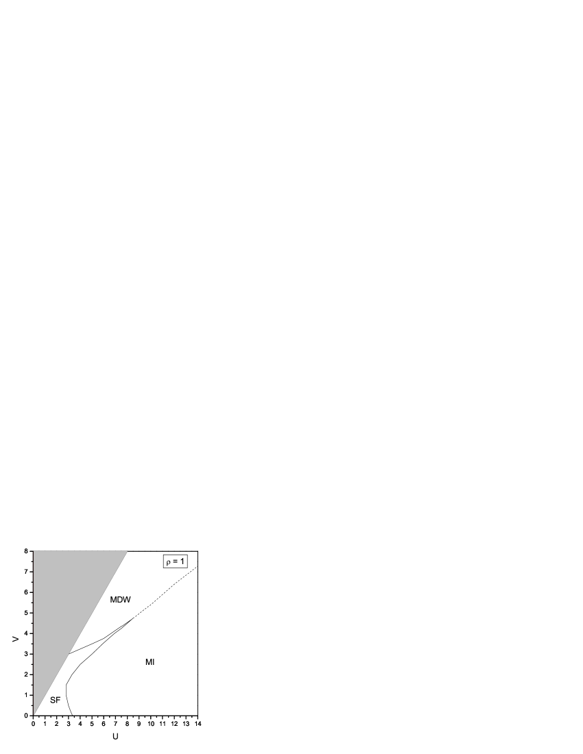
Figure 1: The FSDMRG phase diagram of the one-dimensional, extended Bose-Hubbard model for density $\rho=1$ showing SF, MI, and MDW phases. The two full lines indicate continuous transitions whereas the dashed line is a first-order boundary; these meet at a bicritical point. We do not consider the shaded region $V>U$.

The remaining part of this paper is organized as follows. Section II contains the details of our Finite-size Density-Matrix Renormalization Group (FSDMRG) calculation. Section III contains our results. We end with concluding remarks in Section IV.

II FSDMRG Calculations

The Finite-Size Density-Matrix Renormalization Group (FSDMRG) method has proven to be very useful in studies of one-dimensional quantum systems rvpai ; white ; rvpai_cnr . To make this paper self-contained we summarize the salient points of this method. Open boundary conditions are preferred for such calculations since the loss of accuracy with increasing system size is much less than in the case of periodic boundary conditions. The conventional FSDMRG method consists of the following two steps:

1. The infinite-system density-matrix renormalization group method (DMRG), where we start with a system with four sites, add two sites at each step of the iteration, and continue till we obtain a system with the desired number $L$ of sites ( in most of our calculations we use $L\simeq 100$ but, in some representative cases, we have gone up to $L=200$).

2. The finite-system method in which the system size $L$ is held fixed, but the energy of a target state is improved iteratively by a sweeping procedure, described below, till convergence is obtained.

For a model like Eq. (1) we first construct the Hamiltonian matrix of the superblock configuration ${\bf B}^{\ell}_{1}\bullet\bullet~{}{\bf B}^{r}_{1}$, where ${\bf B}^{\ell}_{1}$ and ${\bf B}^{r}_{1}$ represent left- and right-block Hamiltonians, respectively, and each one of the $\bullet$ represents a single-site Hamiltonian. In the first step of the DMRG iteration both ${\bf B}^{\ell}_{1}$ and ${\bf B}^{r}_{1}$ also represent single sites, so, at this step, we have a four-site chain. We now diagonalize the Hamiltonian matrix of the superblock and obtain the energy and the eigenfunction of a target state. In our study the target state is the ground state of the system of size $L$ with either $N=L$ or $N=L\pm 1$ bosons. The latter is required for obtaining the gap in the energy spectrum. We now divide the superblock into two equal halves, the left and the right parts, which are treated, respectively, as the system and the universe. The density matrix for this system, namely, ${\bf B}^{\ell}_{2}\equiv{\bf B}^{\ell}_{1}~{}\bullet$, is calculated from the target state. If we write the target state as $\mid\psi\rangle=\sum_{i,j}\psi_{i,j}\mid i\rangle\mid j\rangle$, where $\mid i\rangle$ and $\mid j\rangle$ are, respectively, the basis states of the system and the universe, then the density matrix for the system has elements $\rho_{i,i^{\prime}}=\sum_{j}\psi_{i,j}\psi_{i^{\prime},j}$. The eigenvalues of this density matrix measure the weight of each of its eigenstates in the target state. The optimal states for describing the system are the ones with the largest eigenvalues of the associated density matrix. In this first step of the DMRG the superblock, and hence the dimension of the density matrix, is small, so all the states can be retained. However, in subsequent steps, when the sizes of the superblocks and density matrices increase, only the most significant states are retained, say the ones corresponding to the largest $M$ eigenvalues of the density matrix (in our studies we choose $M=128$). We then obtain the effective Hamiltonian for the system ${\bf B}^{\ell}_{2}$ in the basis of the significant eigenstates of the density matrix; this is used in turn as the left block for the next DMRG iteration. In the same manner we obtain the effective Hamiltonian for the right block, i.e., ${\bf B}^{r}_{2}\equiv\bullet{\bf B}^{r}_{1}$. In the next step of the DMRG we construct the Hamiltonian matrix for the superblock ${\bf B}^{\ell}_{2}\bullet\bullet~{}{\bf B}^{r}_{2}$, so the size of the system increases from $L=4$ to $L=6$. For a system of size $L$, we continue, as in the first step, by diagonalizing the Hamiltonian matrix for the configuration ${\bf B}^{\ell}_{\frac{L}{2}-1}\bullet\bullet{\bf B}^{r}_{\frac{L}{2}-1}$ and setting ${\bf B}^{\ell}_{\frac{L}{2}}\equiv{\bf B}^{\ell}_{\frac{L}{2}-1}\bullet$ and ${\bf B}^{r}_{\frac{L}{2}}\equiv\bullet{\bf B}^{r}_{\frac{L}{2}-1}$ in the next step of the DMRG iteration. Thus at each step of the DMRG iteration the left and right blocks increase in length by one site and the total length $L$ of the chain increases by $2$.

In the infinite-system DMRG method outlined above the left- and right-block bases are not optimized in the following sense: The DMRG estimate for the target-state energy, at the step when the length of the system is $L$, is not as close to the exact value of the target-state energy for this system size as it can be. It has been found that the FSDMRG method overcomes this problem white . In this method we first use the infinite-system DMRG iterations to build up the system to a certain desired size $L$. The $L$-site superblock configuration is now given by ${\bf B}^{\ell}_{\frac{L}{2}-1}\bullet~{}\bullet~{}{\bf B}^{r}_{\frac{L}{2}-1}$. In the next step of the FSDMRG method, the superblock configuration ${\bf B}^{\ell}_{\frac{L}{2}}~{}\bullet~{}\bullet~{}{\bf B}^{r}_{\frac{L}{2}-2}$, which clearly keeps the system size fixed at $L$, is used. This step is called sweeping in the right direction since it increases (decreases) the size of the left (right) block by one site. For this superblock the system is ${\bf B}^{\ell}_{\frac{L}{2}}\bullet$, the universe is $\bullet{\bf B}^{r}_{\frac{L}{2}-2}$, the associated density matrix can be found, and from its most significant states the new effective Hamiltonian for the left block, with $(\frac{L}{2}+1)$ sites, is obtained. We sweep again, in this way, to obtain a left block with $(\frac{L}{2}+2)$ sites and so on till the left block has $(L-3)$ sites and the right block has 1 site so that, along with the two sites in between these blocks, the system still has size $L$; or, if a preassigned convergence criterion for the target-state energy is satisfied, this sweeping can be terminated earlier. Note that, in these sweeping steps, for the right block we need ${\bf B}^{r}_{1}$ to ${\bf B}^{r}_{L-3}$, which we have already obtained in earlier steps of the infinite-system DMRG. Next we sweep leftward: the size of the left (right) block decreases (increases) by one site at each step. Furthermore, in each of the right- and left- sweeping steps, the energy of the target state decreases systematically till it converges (we use a six-figure convergence criterion in our calculations).

We use a slightly modified form of the FSDMRG method in which we sweep, as described above, at every step of the DMRG scheme and not only in the one that corresponds to the largest value of $L$. This helps in obtaining accurate $\beta$ functions which we use to obtain critical exponents (see below) at continuous transitions. Furthermore, since the superfluid phase in models such as Eq. (1), in $d=1$ and at $T=0$, is critical and has a correlation length that diverges with the system size $L$, finite-size effects must be removed by using finite-size scaling as we show below. For this purpose, the energies and correlation functions, obtained from a DMRG calculation, should have converged properly for each system size $L$. It is important, therefore, that we use the FSDMRG method as opposed to the infinite-system DMRG method especially in the vicinities of continuous phase transitions. We find that convergence, to a specified accuracy for the target-state energy, is faster in the MI phase than in the SF phase. Figure (2) shows, at a representative point in the SF phase of Fig. (1), how the percentage disagreement between DMRG and FSDMRG ground-state energies increases with $L$ in our calculations.

Figure 2: The percentage difference between the ground state energies $\Delta E_{L}=(E^{DMRG}_{L}-E^{FSDMRG}_{L})/E^{FSDMRG}_{L}$ obtained by DMRG and FSDMRG methods, for a representative point in the SF phase of Fig (1), plotted as a function of $L$.

Since the bases of left- and right-block Hamiltonians are truncated by neglecting the eigenstates of the density matrix corresponding to small eigenvalues, this leads to truncation errors. If we retain $M$ states, the density-matrix weight of the discarded states is $P_{M}=\sum_{\alpha=1}^{M}(1-\omega_{\alpha})$, where $\omega_{\alpha}$ are the eigenvalues of density matrix. $P_{M}$ provides a convenient measure of the truncation errors. We find that these errors depend on the order-parameter correlation length in a phase. For a fixed $M$, we find very small truncation errors in the MI and MDW phases; these grow as the MI-SF and MDW-SF transitions are approached; and the truncation errors are largest in the SF phase. In our calculations we choose $M$ such that the truncation error is always less than $5\times 10^{-6}$; we find that $M=128$ suffices.

The number of possible states per site in the Bose-Hubbard model is infinite since there can be any number of bosons on a site. In a practical DMRG calculation we must restrict the number $n_{max}$ of states or bosons allowed per site. The smaller the interaction parameters $U$ and $V$, the larger must $n_{max}$ be. As in earlier calculations rvpai ; kuhner ; rvpai_cnr on related models, we find that $n_{max}=4$ is sufficient for the values of $U$ and $V$ considered here; we have checked in representative cases that our results do not change significantly if $n_{max}=5$.

In summary, then, our FSDMRG procedure gives us the energy $E_{L}(N)$ for the ground state of model (1) and the associated eigenstate $\mid\psi_{0LN}\rangle$. Given these we can calculate the energy gaps, order parameters, and correlation functions that characterize all the phases of this model and thence the phase diagram. We discuss this in Section III.

III Results

The single-particle energy gap $G_{L}$ for a system of size $L$, the order parameter for the MDW phase, and the correlation functions that characterize SF and MDW phases in model (1) can be defined in a straightforward manner in terms of the energies and wavefunctions mentioned in the previous Section. The energy gap is

$$G_{L}=E_{L}(N+1)+E_{L}(N-1)-2E_{L}(N),$$ (3)

where $E_{L}(N)$ is the ground-state energy for a system of size $L$ with $N$ bosons; since we are interested in studying the case $\rho=1$, we increase the number of bosons by 2 at every DMRG step in which 2 sites are added to the system (Sec. II) so that $\rho=N/L=1$. We expect, and show explicitly below, that this gap is positive in both MI and MDW phases, which are incompressible insulators, but it vanishes in the SF phase, which is compressible.

The correlation function that characterizes the SF phase is

$$\Gamma_{L}^{SF}(r)\equiv\langle\psi_{0LN}|a_{0}^{\dagger}a_{r}|\psi_{0LN}\rangle,$$ (4)

where $|\psi_{0LN}\rangle$ is the ground-state wavefunction of the system with size $L$ and $N$ bosons. The associated correlation length can be obtained from the second moment of this correlation function, namely,

$$\xi^{SF}_{L}\equiv\left[\frac{\sum_{r}r^{2}\Gamma_{L}^{SF}(r)}{\sum_{r}\Gamma_{L}^{SF}(r)}\right]^{1/2}.$$ (5)

Note that $\xi^{SF}_{L}$ is the correlation length for SF ordering in a system of size $L$; it remains finite so long as $L<\infty$.

The MDW phase can be differentiated from the MI phase by using the order parameter for the MDW phase

$$M_{MDW}=\frac{1}{L}\sum_{i}(-1)^{i}\langle\psi_{0LN}|(\hat{n}_{i}-\rho)|\psi_{0LN}\rangle,$$ (6)

and the associated correlation function

$$\Gamma_{L}^{MDW}(r)\equiv\langle\psi_{0LN}|(\hat{n}_{0}-\rho)(\hat{n}_{r}-\rho)|\psi_{0LN}\rangle;$$ (7)

the correlation length for MDW ordering $\xi^{MDW}_{L}$ can be defined as in Eq. (5) but with $\Gamma_{L}^{MDW}$ instead of $\Gamma_{L}^{SF}$.

It is useful first to discuss the case $V=0$. Here we reproduce the well-understood SF-MI transition. In $d=1$ the appearance of the SF phase is signaled by the divergence of the correlation length $\xi^{SF}_{L\to\infty}$. For a finite system $\xi^{SF}_{L}$ is finite and we must extrapolate to the $L\rightarrow\infty$ limit, which is best done by using finite-size scaling. In the critical region the correlation length

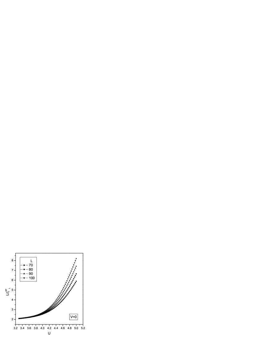
Figure 3: $L/\xi_{L}^{SF}$ plotted as a function of $U$ for different system sizes and $V=0$ in model (1). The coalescence of different curve for $U\simeq 3.4$ shows a Kosterlitz-Thouless-type SF-MI transition.

$$[\xi^{SF}_{L}]^{-1}\approx L^{-1}f(L/\xi^{SF}_{\infty}),$$ (8)

where the scaling function $f(x)\sim x,\,x\to 0$. Thus plots of $L/\xi^{SF}_{L}$ versus $U$, for different system sizes $L$, consist of curves that intersect at the critical point at which the correlation length for $L=\infty$ diverges. Such plots are given in Fig. (3) for $V=0$. Curves for different values of $L$ coalesce for $U\leq U_{c}\simeq 3.4$ indicating the existence of a critical SF phase, with a diverging correlation length, i.e., a power-law decay of correlations, for all $0\leq U\leq U_{c}$. The single-particle gap $G_{L}$ scales as the inverse of this correlation length and is, therefore, zero for $L=\infty$ for $0\leq U\leq U_{c}$. For $U>U_{c}$ we have an MI phase with a finite correlation length and a nonzero gap. Figure (3) also suggests that the SF-MI transition here is of the KT type. We can quantify this by calculating the $\beta$ function at this transition via the Roomany-Wyld (RW) approximants rvpai ; roomany ; barber

$$\beta_{LL^{\prime}}=\frac{1-\ln(\xi_{L}^{SF}/\xi_{L^{\prime}}^{SF})/\ln(L/L^{\prime})}{(\xi_{L}^{SF}\xi_{L^{\prime}}^{SF}/\xi^{\prime}_{L}{\xi^{\prime}}_{L^{\prime}})^{1/2}},$$ (9)

where $L$ and $L^{\prime}$ denote two system sizes and $\xi^{\prime}_{L}\equiv d\xi_{L}^{SF}/dU$. For a KT transition the correlation length $\xi_{\rm{KT}}\sim\exp(c/(U-U_{c})^{\sigma})$ and $\beta\sim(U-U_{c})^{1+\sigma}$, with $\sigma=1/2$.

Figure 4: The $\beta$ function for the MI-SF transition for $V=0$ obtained by using RW approximants [Eq. (9)] with $L=98$ and $L^{\prime}=100$. The full line is a fit to the form $\beta(U)=c(U-U_{c})^{(1+\sigma)}$; we get $c=0.37\pm 0.01$, $U_{c}=3.35\pm 0.02$ and $\sigma=0.48\pm 0.05$.

In Fig. (4) we show the $\beta$ function for the SF-MI transition for $V=0$. To obtain this $\beta$ function we use $L=98$ and $L^{\prime}=100$ in Eq. (9). Our fit to the data of Fig. (4) yields $U_{c}=3.35\pm 0.02$ and $\sigma=0.48\pm 0.05$ which are consistent with the values reported earlier rvpai ; kuhner . If we fit our data (here and below) over a fixed region of $(U-U_{c})/U_{c}$, then our nonlinear least-squares programme yields smaller errors. The conservative error bars we quote here reflect the range over which our fitted values for $U_{c}$, $\sigma$, etc., vary when we change the region of $(U-U_{c})/U_{c}$ over which we fit our data, namely, $0.001<|U-U_{c}|/U_{c}<0.2$ or $0.001<|U-U_{c}|/U_{c}<0.35$.

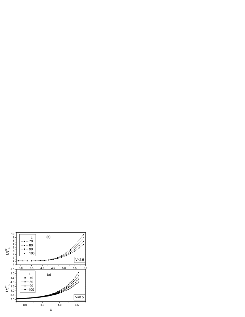
Figure 5: $L/\xi_{L}^{SF}$ plotted as a function of $U$ for different system sizes and for (a) $V=0.5$ and (b) $V=2.5$ in model (1). The coalescence of different curve for $U<3.0$ in (a) and $U<4.2$ in (b) show KT-type SF-MI transitions.

Initially the nearest-neighbor interaction $V$ suppresses the SF phase relative to the MI phase, but at larger values of $V$ this trend is reversed leading to a reentrant SF [Fig. (1)]. Figure (5a) shows a plot of $L/\xi_{L}^{SF}$ versus $U$ for $V=0.5$; by comparing this with Fig. (3) we see that $U_{c}(V=0.5)<U_{c}(V=0)$. Curves for different values of $L$ coalesce for $U\leq U_{c}(V=0.5)\simeq 3.0$ indicating a power-law SF phase, as for $V=0$, and a KT-type MI-SF transition. Again we use RW approximants to obtain the $\beta$ function shown in Fig. (6) and our numerical fit yields $U_{c}=2.95\pm 0.02$ and $\sigma=0.53\pm 0.05$. Eventually the MI-SF phase boundary in Fig. (1) turns back; a representative plot of $L/\xi_{L}^{SF}$ versus $L$, for $V=2.5$, illustrates this [Fig. (5b)]; we find $U_{c}(V=2.5)\simeq 4.2$. This reentrance of the SF phase, with increasing $V$, was not resolved by the study of Ref. [niyaz, ].

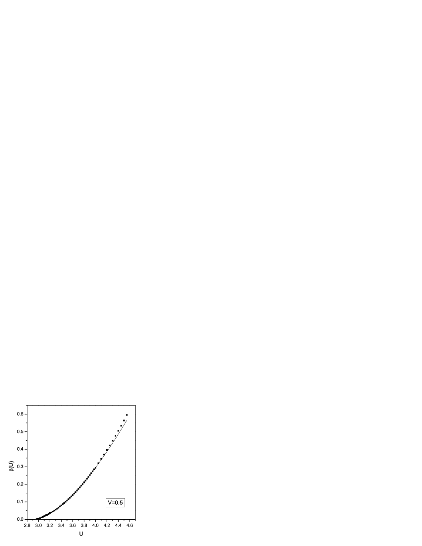
Figure 6: The $\beta$ function of the MI-SF transition for $V=0.5$, obtained by using the RW approximants with $L=98$ and $L^{\prime}=100$ as in Fig. (4). The full line is a fit to the form $\beta(U)=c(U-U_{c})^{(1+\sigma)}$; we get $c=0.27\pm 0.01$, $U_{c}=2.95\pm 0.02$ and $\sigma=0.53\pm 0.05$.

For sufficiently large values of $V$ we can have an MDW phase and an SF-MDW transition, at small values of $U$, and an MI-MDW transition at large values of $U$ as shown in the phase diagram of Fig. (1). In Fig. (7) we plot the MDW order parameter $M_{MDW}$ as a function of $1/L$ for $U=6$ and values of $V$ ranging from $V=3.0$ to $5.3$ in steps of $0.1$. We see that $M_{MDW}$ goes to zero for $V<V_{c}(U=6)\simeq 3.9$ whereas it is nonzero for higher values of $V$.

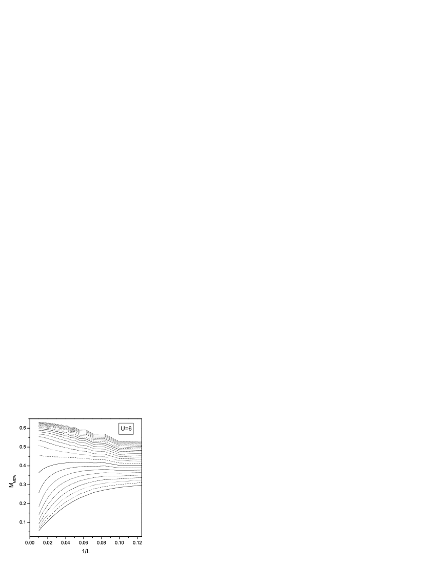
Figure 7: The MDW order parameter $M_{MDW}$ versus $1/L$ for $U=6$ and different values of $V$ starting from $3.0$ below to $5.3$ above in steps of $0.1$.

To determine the universality classes of the MI-SF and SF-MDW transitions we plot in Fig. 8 both the order parameter $M_{MDW}$ and $L/\xi^{SF}_{L}$ as functions of $V$ for $U=6$. The different curves for $L/\xi^{SF}_{L}$ coalesce in the region $3.5\lesssim U\lesssim 3.9$ indicating an SF phase sandwiched between MI and MDW phases. Both SF-MI and SF-MDW transitions are continuous. To confirm this we have also obtained plots of the ground-state energy $E_{0}\equiv\lim_{L\to\infty}E_{L}(N)$ as a function of $V$ for fixed $U$. In Fig. (9) we plot $E_{0}$ and $dE_{0}/dV$ versus $V$; this plot shows no discontinuity at the SF-MI and SF-MDW transitions (as it does at the first-order MI-MDW transition discussed below for $U=12$).

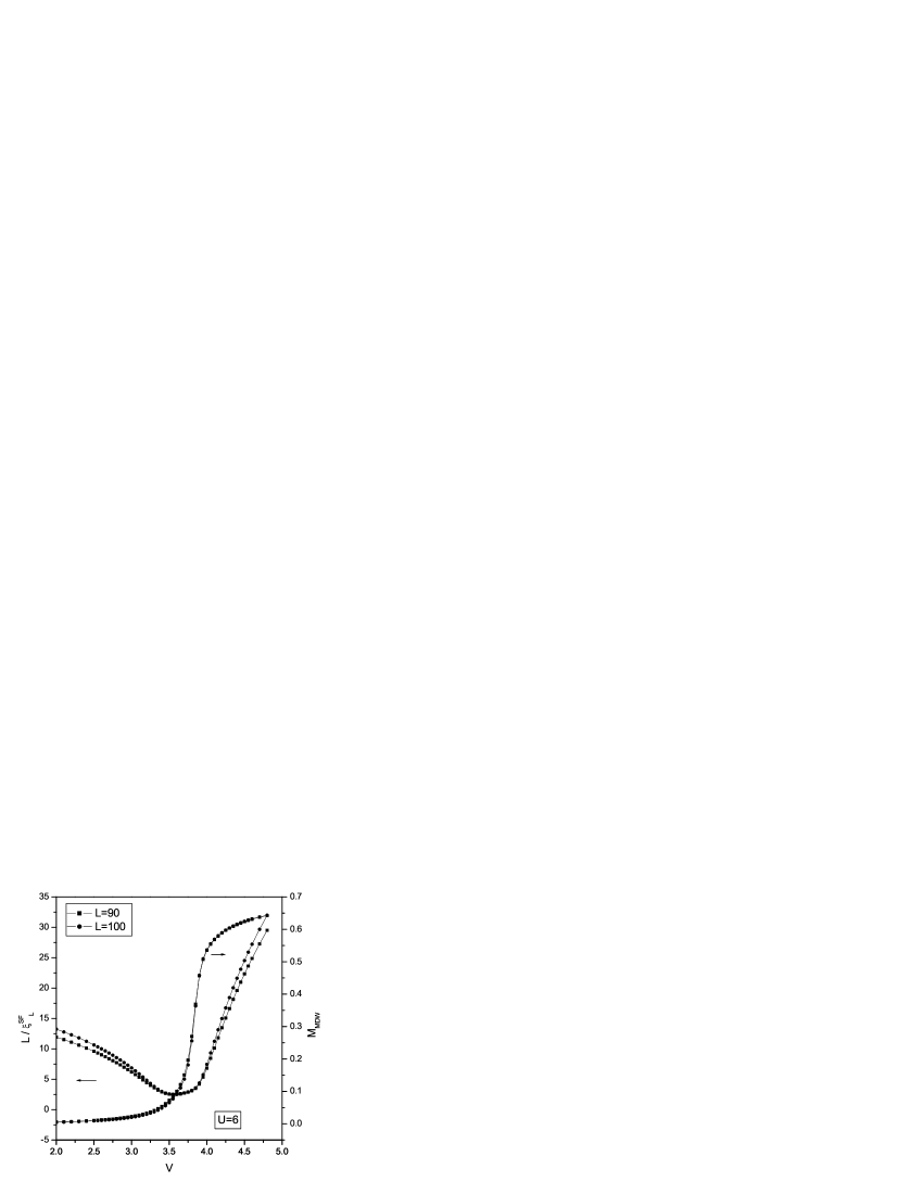
Figure 8: Plots of $L/\xi^{SF}_{L}$ and $M_{MDW}$ versus $V$ for $U=6$ and $L=90$ and $100$. The coalescence of different curves of $L/\xi^{SF}_{L}$, for $3.5<V<3.9$, shows an SF phase sandwiched between MI and MDW phases; for $3.9\lesssim V$ we obtain the MDW phase with $M_{MDW}>0$.

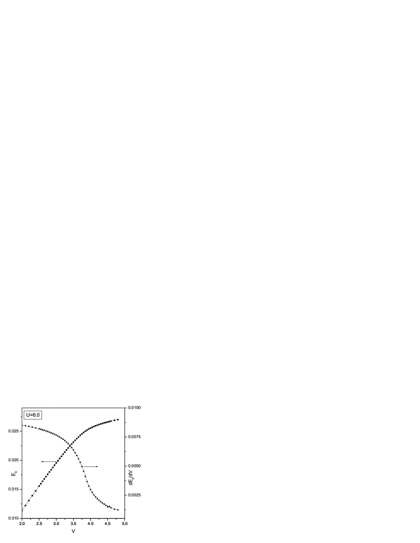
Figure 9: Plots of the ground-state energy $E_{0}$ and its derivative $dE_{0}/dV$ versus $V$ for $U=6$. There is no visible discontinuity in $dE_{0}/dV$ so both MI-SF and SF-MDW transitions are continuous.

To determine the universality classes of these SF-MI and SF-MDW transitions we have obtained $\beta$ functions, via RW approximants for $\xi^{SF}_{L}$, in Fig. (10) for $U=6.0$. For the MI-SF transition, we get $V_{c}=3.59\pm 0.05$ and $\sigma=0.47\pm 0.05$; and, for the SF-MDW transition, $V_{c}=3.78\pm 0.05$ and $\sigma=0.49\pm 0.05$. Thus both of these transitions are of the KT type. However, in addition, the MDW-SF transition also has an Ising character (two-dimensional) since the MDW phase has a doubly degenerate ground state as mentioned above. To extract such Ising-model exponents, we use the form $M_{MDW}\sim(V-V_{c})^{\beta_{MDW}}$ as $V\downarrow V_{c}$, where $\beta_{MDW}$ is the MDW order-parameter exponent. For $U=6$ our fit yield $V_{c}=3.87\pm 0.05$ and $\beta_{MDW}=0.12\pm 0.01$ (Fig. 11) in good agreement with the two-dimensional, Ising order parameter exponent. Note that the value of $V_{c}$ obtained from this fit for $M_{MDW}$ is within error bars of that obtained from the $\beta$ function for the SF-MDW transition. Thus, within our calculation we cannot resolve a supersolid phase which has long-range SF correlations and MDW ordering.

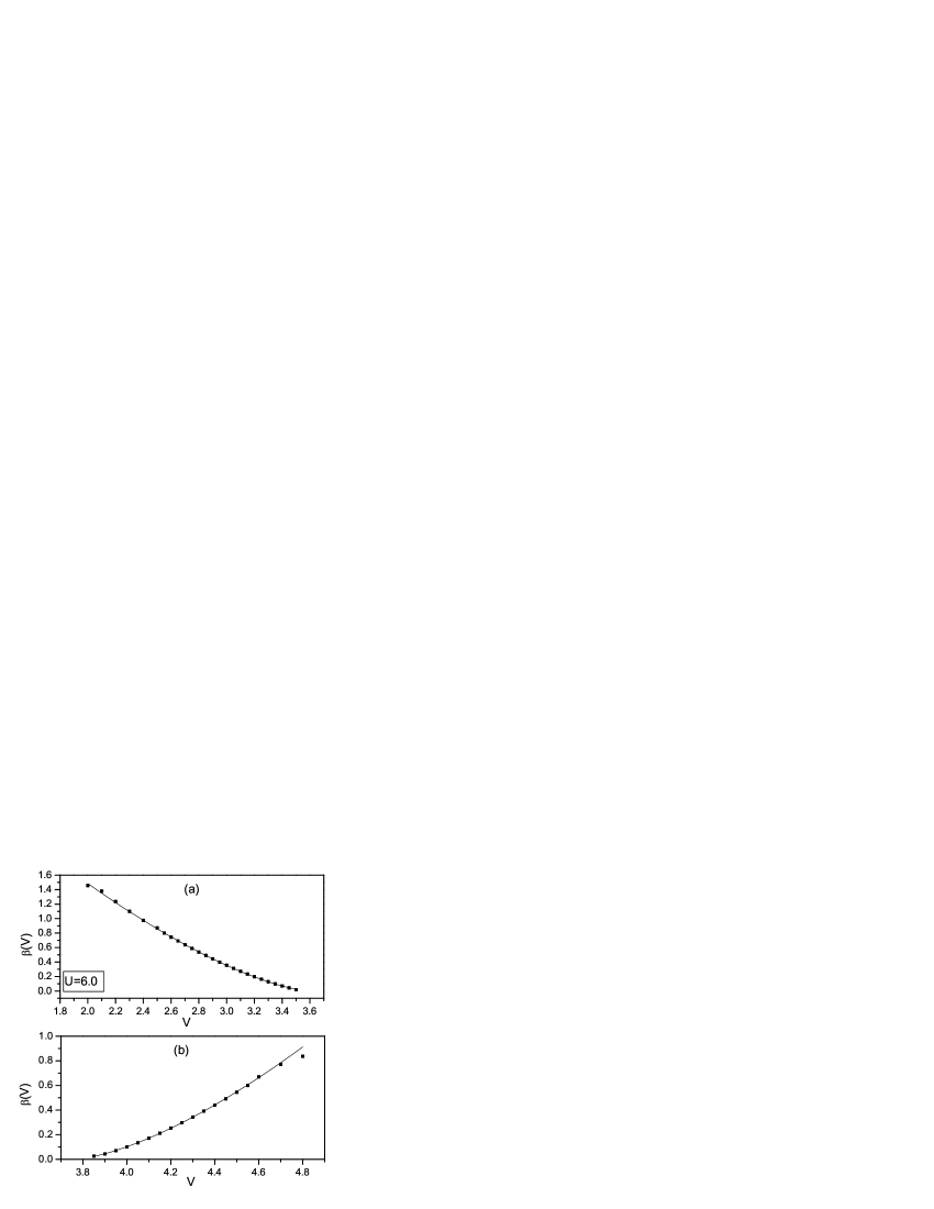
Figure 10: The $\beta$ functions for MI-SF (a) and MDW-SF (b) transition for $U=6$, obtained by using RW approximants with $L=98$ and $L^{\prime}=100$. The full line is a fit to the form $\beta(U)=c(U-U_{c})^{(1+\sigma)}$. For the MI-SF transition (a) we get $c=0.76\pm 0.01$, $U_{c}=3.59\pm 0.05$ and $\sigma=0.47\pm 0.05$ and for the MDW-SF transition (b) we get $c=0.86\pm 0.01$, $U_{c}=3.78\pm 0.05$ and $\sigma=0.49\pm 0.05$.

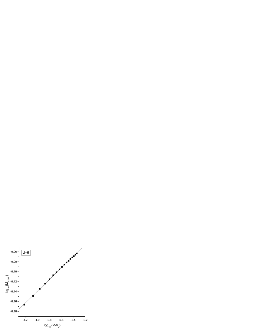
Figure 11: A log-log plot (base 10) of the MDW order parameter $M_{MDW}$ versus $V-V_{c}$ for $U=6$. The straight line is a fit to the form $M_{MDW}\sim(V-V_{c})^{\beta_{MDW}}$, $V\downarrow V_{c}$. Our fit yields $V_{c}=3.87\pm 0.05$ and $\beta_{MDW}=0.12\pm 0.01$.

From the phase diagram of Fig. (1) we see that, for sufficiently large values of $U$, there is no SF phase and only a direct, first-order MI-MDW transition. This direct transition shows up clearly in Fig. 12 where we plot $L/\xi_{L}^{SF}$ and $M_{MDW}$ versus $V$ for $U=12$: Curves of $L/\xi_{L}^{SF}$, for different values of $L$, do not merge at any point, so we can conclude that no power-law SF phase intervenes between MI and MDW phases. Furthermore, the sharp jump in $M_{MDW}$ at $V\simeq 6.3$ indicates that we have a first-order MI-MDW transition. This is corroborated by the plots of the ground-state energy $E_{0}$ and its derivative $dE/dV$ given in Fig. 13 for $U=12$; the discontinuity of $dE/dV$ at $V\simeq 6.3$ indicates the first-order nature of the transition.

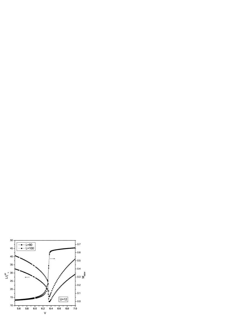
Figure 12: Plots of $L/\xi_{L}^{SF}$ and $M_{MDW}$ versus $V$ for $U=12$ and different system sizes $L$. Note that the curves for $L/\xi_{L}$ do not meet at any point; however, $M_{MDW}$ jumps at the first-order, MI-MDW transition at $V\simeq 6.3$.

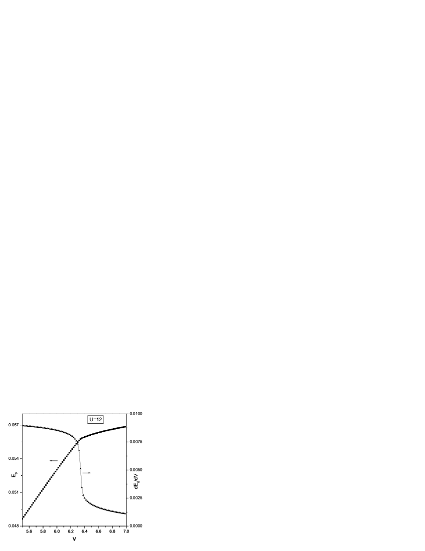
Figure 13: The ground-state energy $E_{0}$ and its derivative $dE_{0}/dV$ versus $V$ for $U=12.0$; the jump in $dE_{0}/dV$ at $V\simeq 6.3$ shows that the MI-MDW transition is first order.

The only feature of the phase diagram of Fig. (1) that remains unexplored now is the region in which the continuous MI-SF and SF-MDW phase boundaries meet the first-order MI-MDW boundary. The simplest topology possible here is that these meet at one bicritical point. Our data are not inconsistent with such a topology. Figure (14) shows, via plots of $L/\xi^{SF}_{L}$ versus $V$, for different values of $L$ and $U$, how the extent of the SF phase (the region over which the curves of $L/\xi^{SF}_{L}$ coalesce) shrinks as we approach the bicritical point. Similarly Fig. (15) shows how the jump in $M_{MDW}$ across the MI-MDW first-order transition decreases as we approach the bicritical point. To confirm that this is indeed the topology of the phase diagram in the region where the MI-SF, SF-MDW, and MI-MDW phase boundaries meet, we must obtain the critical exponents in the vicinity of the bicritical point. This is beyond the accuracy of our calculation at the moment. Nor can we rule out completely more complicated topologies of phase diagrams in which very closely spaced tricrital points and critical endpoints are used to link the three phase boundaries we have studied above.

Figure 14: Plots of $L/\xi_{L}^{SF}$ versus $V$ for different values of $U$ and different system sizes $L(80,90,100)$. The region over which curves for different values of $L$ coalesce decreases as we go from $U=8$ to $U=8.5$; and there is no coalescence for $U=9$. This shows how the SF phase shrinks as we approach the bicritical point.

Figure 15: The MDW order parameter $M_{MDW}$ plotted versus $V/V_{c}$ for different values of $U$ across the MI-MDW first-order transition. The jump in $M_{MDW}$ at the first-order phase boundary decreases as we approach the bicritical point at ($U,V)=(8.5\pm 0.05,4.75\pm 0.05)$.

IV Conclusions

We have carried out an extensive study of the one-dimensional, extended Bose-Hubbard model (1) by using the FSDMRG method. Our study yields ground-state energies, single-particle gaps, the MDW order parameter, and SF correlation functions and correlation lengths. By studying these we obtain an accurate phase diagram [Fig. (1)] for this model. This shows continuous MI-SF and SF-MDW transitions meeting the first-order MI-MDW boundary at a bicritical point.

We have looked for, but not found, a supersolid (SS) phase which, in the context of the lattice model we study here, would exhibit power-law superfluid correlations, as in the SF phase, and a nonzero order parameter $M_{MDW}$, as in the MDW phase. It is likely frey that further than nearest-neighbor interactions will be required to stabilize the SS phase as we will explore elsewhere.

We hope our detailed study of model (1) will stimulate experimental studies. A recent experimental study stoferle has shown that it is possible, by a suitable choice of confining potentials in optical lattices, to obtain a physical realization of the one-dimensional Bose-Hubbard models. It would be interesting to see how nearest-neighbor interactions, like $V$, can be obtained in such lattices. If this can be done, the rich phase diagram of Fig. (1) can be explored experimentally.

- (1) M. Ma, B. I. Halperin, and P. A. Lee, Phys. Rev. B 34 3136 (1989); P. Nisamaneephong, L. Zhang, and M. Ma, Phys. Rev. Lett. 71 3830 (1993).
- (2) M. P. A. Fisher, P. B. Weichman, G. Grinstein and D. S. Fisher, Phys. Rev. B 40 546 (1989).
- (3) W. Krauth, M. Caffarel, and J. P. Bouchaud, Phys. Rev. B 45 3137 (1992).
- (4) K. Sheshadri, H. R. Krishnamurthy, R. Pandit, and T. V. Ramakrishnan, Europhys. Lett. 22 257 (1993); Phys. Rev. Lett. 75 4075 (1995).
- (5) T. V. Ramakrishnan, Ordering Disorder: Prospect and Retrospect in Condensed Matter Physics, eds. V. Srivastava, A. K. Bhatnagar and D. G. Naugle AIP Conference Proceedings 286 38 (1994) and references therein.
- (6) L. Amico and V. Penna, Phys. Rev. Lett. 80 2189 (1998).
- (7) R. V. Pai, R. Pandit, H. R. Krishnamurthy and S. Ramasesha, Phys. Rev. Lett. 76 2937 (1996).
- (8) R. Baltin and K. H. Wagenblast, Europhys. Lett. 39 7 (1997).
- (9) T. D. Kühner and H. Monien, Phys. Rev. B 58 R14741 (1998), T. D. Kühner, S. R. White and H. Monien H, Phys. Rev. B 61 12474 (2000).
- (10) V. A. Kashurnikov and B. V. Svistunov, Phys. Rev. B. 53 11776 (1996).
- (11) G. G. Batrouni, R. T. Scalettar, G. T. Zimanyi and A. P. Kampf, Phys. Rev. Lett. 74 2527 (1995); P. Niyaz, R. T. Scalettar, C. Y. Fong and G. G. Batrouni, Phys. Rev. B. 44 7143 (1991).
- (12) W. Krauth, N. Trivedi, and D. Ceperley, Phys. Rev. Lett. 67 2307 (1991); N. Trivedi and M. Makivic, Phys. Rev. Lett. 74 1039 (1995).
- (13) M. Wallin, E. S. Sorensen, S. M. Girvin, and A. P. Young, Phys. Rev. B 49 12115 (1994).
- (14) S. Zhang, N. Kawashima, J. Carlson, and J. E. Gubernatis, Phys. Rev. Lett. 74 1500 (1995).
- (15) M. H. W. Chan, K. I. Blum, S. Q. Murphy, G. K. S. Wong, and J. D. Reppy, Phys. Rev. Lett. 61 1950 (1988).
- (16) E. Chow, P. Delsing and D. B. Haviland, Phys. Rev. Lett 81 204 (1998).
- (17) A. van Oudenaarden, and J. E. Mooij, Phys. Rev. Lett. 76 4947 (1996); A. van Oudenaarden, B. van Leeuwen, M. P. M. Robbens and J. E. Mooij, Phys. Rev. B 57 11684 (1998).
- (18) D. B. Haviland, Y. Liu, and A. M. Goldman, Phys. Rev. Lett. 62 2180 (1989).
- (19) D. R. Nelson and V. M. Vinokur, Phys. Rev. B 48 13060 (1993).
- (20) M. Greiner, O. Mandel, T. Esslinger, T. W. Hänsch and L. Bloch Nature (London) 415 39 (2002).
- (21) D. Jaksch, C. Bruder, J. I. Cirac, C. W. Gardiner and P. Zoller, Phys. Rev. Lett. 81 3108 (1998).
- (22) E. Kim and M. H. W. Chan, Nature (London) 427 225 (2004).
- (23) J. M. Kosterlitz and D. J. Thouless, J. Phys. C 6, 1181 (1973).
- (24) R. J. Baxter, Exactly Solved Models in Statistical Mechanics, (Academic-Press, New York, 1982).
- (25) S. R. White, Phys. Rev. Lett. 69 2863 (1992); Phys. Rev. B. 48 10345 (1993).
- (26) P. Niyaz, R. T. Scalettar, C. Y. Fong and G. G. Batrouni, Phys. Rev. B. 50 362 (1994).
- (27) E. Jeckelmann, Phys. Rev. Lett. 89 236401 (2002).
- (28) R. V. Pai and R. Pandit, Proc. Indian Academy of Sciences (Chemical Sciences) 115 721 (2003).
- (29) H. H. Roomany and H. W. Wyld, Phys. Rev. D 21 3341 (1980).
- (30) M. N. Barber, Phase Transition and Critical Phenomena, eds. C. Domb C. and J. L. Lebowitz, 8 (Academic, New York) 145 (1990).
- (31) E. Frey and L. Balents, Phys. Rev. B 55 1050 (1997).
- (32) T. Stöferle, H. Moritz, C. Schori, M. Köhl and T. Esslinger, Phys. Rev. Lett. 92 130403 (2004).