]June 30 , 2004

Signatures of spin-charge separation in scanning probe microscopy

Abstract

We analyze the effect of an auxiliary scatterer, such as the potential of a scanning tip, on the conductance of an interacting one-dimensional electron system. We find that the differential conductance for tunneling into the end of a semi-infinite quantum wire reflects the separation of the elementary excitations into spin and charge modes. The separation is revealed as a specific pattern in the dependence of the conductance on bias and on the position of the scatterer.

Interaction between electrons has a profound effect on the properties of one-dimensional electron systems. Basic notions of Fermi liquid theory are no longer applicable, as is manifested, e.g., in the absence of well-defined fermionic quasiparticles related to the non-interacting state. Instead, the low-energy physics of these systems is described by the concept of a Luttinger liquid haldane .

One consequence of the inter-electron interaction is the separation of elementary excitations into two branches with different velocities, corresponding to spin and charge excitations. This spin-charge separation is apparent already within the random-phase approximation treatment of the interaction. The relation between the bare electron degrees of freedom and the elementary excitations of a Luttinger liquid, manifested in the suppression of the electron density of states at low energies review , requires more sophisticated techniques such as bosonization haldane .

The suppression of the density of states was demonstrated in several tunneling experiments bockrath ; yao . In contrast, the separation into spin and charge modes has proved harder to observe. The simplest idea, to measure the charge- and spin-density response functions, is problematic because coupling to the spin mode is difficult. Another approach is provided by electron tunneling experiments, either into a nearby two-dimensional electron gas (2DEG) altland ; si , or into a second one-dimensional system ophir ; yaroslav ; zulicke ; balents . The latter experiment was recently carried out by Auslaender et al. in quantum wires grown in a GaAs heterostructure ophir ; yaroslav . In these experiments, the differential conductance was measured as a function of voltage and applied magnetic field. Patterns of oscillations in the measured conductance, arising from finite size effects, showed modulations which provide evidence for spin-charge separation in the two wires yaroslav . Another possibility is to use scanning tunneling microscopy (STM) to measure the local density of states, close to the edge of the system eggert1 , in a finite system eggert2 , or next to an impurity kivelson . A difficulty in STM experiments is the need to maintain a small distance between the wire and the tip, necessary for electron tunneling. This is possible in carbon nanotubes; in recent experiments lemay , however, interaction between the electrons was suppressed by the metallic substrate, and the results were adequately interpreted in terms of non-interacting electrons.

A scanning tip may also be placed further away from the wire, thus prohibiting tunneling, but still creating a local potential, which scatters electrons. The conductance of the system may then be measured as a function of tip position. This scanning probe microscopy (SPM) technique was successfully used for imaging the flow of electrons through a quantum point contact in a 2DEG topinka . Similar techniques were also used to image other systems, including confined electrons in a 2DEG crook , multichannel one-dimensional wires ihn , and quantum dots in nanotubes woodside .

In this Letter, we analyze the use of SPM in one dimension. We consider electrons tunneling into a semi-infinite one-dimensional system through a fixed tunnel junction at its end. The scanning tip is used to create a weak potential scatterer along the wire at a distance $x_{0}$ away from its end. The tunneling conductance is then calculated as a function of tip position $x_{0}$. Note the difference from the STM setup (Ref. eggert1 ; kivelson ; eggert2 ) in which the tunneling occurs at the tip position.

We find that the tunneling conductance exhibits oscillations as a function of the applied voltage $V$ and the position $x_{0}$ of the scatterer. The nature of these oscillations depends on the strength of the electron-electron interaction. At moderate or weak interaction, spin-charge separation is readily identifiable as a beating pattern, which allows one to extract the velocities of spin and charge modes. Notably, this information can be extracted from the voltage dependence alone, which may be useful in some experimental setups with a fixed position of the scatterer. At a strong interaction, the dominant contribution oscillates only as a function of $x_{0}$, with wavevector $2k_{F}$ (here $k_{F}$ is the electron Fermi wavevector).

To analyze the effect of an auxiliary scatterer on the current $I$ of electrons which tunnel into the end of a one-dimensional wire, we express the current,

$$I\propto\int d\epsilon\,[n_{F}(\epsilon)-n_{F}(\epsilon+eV)]\,\nu_{\text{lead}}(\epsilon+eV)\,\nu(\epsilon),$$ (1)

in terms of the densities of states $\nu_{\text{lead}}(\epsilon)$ and $\nu(\epsilon)$ of the lead and semi-infinite wire, respectively. Assuming $\nu_{\text{lead}}(\epsilon)$ is essentially energy-independent, the differential conductance $dI/dV$ provides a direct measure of the tunneling density of states at the edge of the wire. The latter is given by

$$\nu(\epsilon)=\frac{1}{4\pi(ik_{F})^{2}}\textrm{Im}\sum_{s}\left.\frac{\partial^{2}}{\partial x\partial x^{\prime}}G^{R}_{s}(x,x^{\prime},\epsilon)\right|_{x=x^{\prime}=0},$$ (2)

where $G_{s}^{R}(x,x^{\prime},\epsilon)$ is the retarded Green function,

$$G_{s}^{R}(x,x^{\prime},\epsilon)=-i\int_{0}^{\infty}dt\,e^{i\epsilon t}\left\langle\left\{\psi_{s}(x,t),\psi_{s}^{\dagger}(x^{\prime},0)\right\}\right\rangle.$$ (3)

Here, we have taken the edge of the wire at $x=0$, and assumed Dirichlet boundary condition, $\psi(0)=0$. We calculate $\nu(\epsilon)$ in the presence of a weak scatterer at $x_{0}$, as a perturbation to the known result for an ideal semi-infinite Luttinger liquid kane-fisher .

Following the standard Luttinger liquid derivation, we bosonize the fermionic operators,

$$\psi_{s}(x)=\frac{1}{\sqrt{2\pi a}}F_{s}\left(e^{-ik_{F}x+i\Phi_{-,s}(x)}-e^{ik_{F}x+i\Phi_{+,s}(x)}\right).$$ (4)

Here, $\Phi_{+,s}$ ($\Phi_{-,s}$) are the bosonic fields corresponding to the right (left) movers, $F_{s}$ is the Klein factor, and $a$ is a short-distance cutoff. The fields $\Phi_{\pm,s}$ are decoupled into charge ($\rho$) and spin ($\sigma$) modes, as well as into their symmetric and anti-symmetric combinations $\vartheta$ and $\varphi$,

$$\Phi_{\pm,s}(x)=\frac{1}{\sqrt{2}}\{\vartheta_{\rho}(x)\pm\varphi_{\rho}(x)+s[\vartheta_{\sigma}(x)\pm\varphi_{\sigma}(x)]\}.$$ (5)

At the barrier, the fields obey the boundary condition $\partial_{x}\vartheta_{\rho}(0)=\partial_{x}\vartheta_{\sigma}(0)=0$, corresponding to the vanishing of the current at the origin. The beauty of the Luttinger liquid formalism is that in terms of the bosonic variables, the Hamiltonian becomes quadratic,

$$H_{0}=\sum_{\nu=\rho,\sigma}\frac{v_{\nu}}{2\pi}\int dx\left[g_{\nu}(\partial_{x}\vartheta_{\nu})^{2}+\frac{1}{g_{\nu}}(\partial_{x}\varphi_{\nu})^{2}\right],$$ (6)

where $v_{\rho}$ ($v_{\sigma}$) is the velocity of the charge (spin) mode, and $g_{\rho}$, $g_{\sigma}$ are the Luttinger liquid parameters. Here, we neglect the interaction in the spin channel. This simplification is possible if the $2k_{F}$ component of the inter-electron interaction potential is weak, or the energy $\epsilon$ is small, as the interaction term is irrelevant under the renormalization flow. In addition, in both cases $g_{\sigma}=1$.

To calculate the tunneling density of states $\nu(\epsilon)$ in perturbation theory, Eqs. (2)–(3) are expressed in terms of time-ordered (and anti-time ordered) Green functions. Using the bosonization formula, Eq. (4), the tunneling density of states is then expressed as

$$\nu(\epsilon)=-\frac{1}{\pi}\sum_{s}\mathrm{Im}\int_{0}^{\infty}dt\,e^{i\epsilon t}\left[\mathcal{G}_{s}(t)-\bar{\mathcal{G}}_{s}(t)\right].$$ (7)

Here, $\mathcal{G}_{s}(t)$ is the time-ordered Green function,

$$\mathcal{G}_{s}(t)=$$

$$-\frac{i}{2\pi a}\left\langle\hat{T}e^{i\left[\vartheta_{\rho}(0,t)+s\vartheta_{\sigma}(0,t)\right]/\sqrt{2}}e^{-i\left[\vartheta_{\rho}(0,0)+s\vartheta_{\sigma}(0,0)\right]/\sqrt{2}}\right\rangle,$$

where $\hat{T}$ is the time-ordering operator. A similar expression holds for the anti-time ordered function $\bar{\mathcal{G}}$.

In absence of the scatterer, the average in Eq. (Signatures of spin-charge separation in scanning probe microscopy) is calculated using the relation $\langle e^{A}e^{B}\rangle_{0}=e^{\langle AB+A^{2}/2+B^{2}/2\rangle_{0}}$ (valid for $A$ and $B$ linear in the fields). Next, the correlation functions are calculated by expressing the fields in terms of the eigenmodes of $H_{0}$,

$$\varphi_{\nu}(x,t)=i\sqrt{g_{\nu}}\!\int_{0}^{\infty}\!\frac{dp}{2\pi}\,c_{p}\sin px\left(a_{p,\nu}e^{-iv_{\nu}pt}\!-\!a^{\dagger}_{p,\nu}e^{iv_{\nu}pt}\right)\!,$$ (9)

$$\vartheta_{\nu}(x,t)=\frac{1}{\sqrt{g_{\nu}}}\!\int_{0}^{\infty}\frac{dp}{2\pi}c_{p}\cos px\left(a_{p,\nu}e^{-iv_{\nu}pt}\!+\!a^{\dagger}_{p,\nu}e^{iv_{\nu}pt}\right)\!,$$ (10)

where $c_{p}=e^{-ap/2}\sqrt{2\pi/p}$. We then have (at $T=0$)

$$\mathcal{G}_{s}^{(0)}(t>0)=-\frac{i}{2\pi a}\prod_{\nu=\rho,\sigma}\left(\frac{a}{a+iv_{\nu}t}\right)^{1/2g_{\nu}},$$ (11)

leading to the known power law dependence of the edge tunneling density of states kane-fisher ,

$$\nu^{(0)}(\epsilon)=\frac{1}{\pi\Gamma\left(\frac{1}{2g}+\frac{1}{2}\right)\sqrt{v_{\sigma}v_{\rho}}}\left(\frac{\epsilon a}{v_{\rho}}\right)^{1/2g-1/2}\,.$$ (12)

Here, we have set $g_{\rho}=g$ and $g_{\sigma}=1$.

The leading correction to $\nu(\epsilon)$ due to an obstacle placed at $x=x_{0}$, is caused by the electron backscattering from it. The backscattering term in the Hamiltonian, which is the one relevant to the calculation, is given by

$$H_{1}=-\frac{U}{2\pi a}\sum_{s}\left(ie^{2ik_{F}x_{0}+i\sqrt{2}\left[\varphi_{\rho}(x_{0})+s\varphi_{\sigma}(x_{0})\right]}+\text{h.c.}\right),$$ (13)

where $U$ is the $2k_{F}$ component of the potential created by the scatterer. We assume $U$ is small, and treat it perturbatively. (The opposite limit of a strong scatterer corresponds to the problem of resonant tunneling through a double barrier, previously studied in detail gornyi ; this limit is not suitable for SPM measurements.)

To linear order in the scatterer strength $U$, one expands the scattering matrix implicit in the definition of the time-ordered Green function (both in the numerator and in the denominator). The correction to the Green function (Signatures of spin-charge separation in scanning probe microscopy) is then given by

$$\mathcal{G}_{s}^{(1)}(t)=-\frac{1}{2\pi a}\int_{-\infty}^{\infty}dt^{\prime}\left\langle\hat{T}e^{i\left[\vartheta_{\rho}(0,t)+s\vartheta_{\sigma}(0,t)\right]/\sqrt{2}}e^{-i\left[\vartheta_{\rho}(0,0)+s\vartheta_{\sigma}(0,0)\right]/\sqrt{2}}\left[H_{1}(t^{\prime})-\left\langle H_{1}(t^{\prime})\right\rangle_{0}\right]\right\rangle_{0}.$$ (14)

Using $\langle e^{A}e^{B}e^{C}\rangle_{0}=e^{\langle AB+AC+BC+(A^{2}+B^{2}+C^{2})/2\rangle_{0}}$, the first order correction to the Green function is

$$\mathcal{G}_{s}^{(1)}(t>0)=-\frac{iU}{(2\pi a)^{2}}\sum_{\pm}\pm e^{\pm 2ik_{F}x_{0}}\left(\frac{a^{2}}{a^{2}+4x_{0}^{2}}\right)^{(g_{\rho}+g_{\sigma})/4}$$

$$\times\int_{-\infty}^{\infty}dt^{\prime}\prod_{\nu=\rho,\sigma}\left(\frac{a}{a+iv_{\nu}t}\right)^{1/2g_{\nu}}\left[\left(\frac{a-ix_{0}\mathrm{sgn}(t-t^{\prime})+iv_{\nu}|t-t^{\prime}|}{a+ix_{0}\mathrm{sgn}(t-t^{\prime})+iv_{\nu}|t-t^{\prime}|}\right)^{\mp 1/2}\left(\frac{a+ix_{0}\mathrm{sgn}(t^{\prime})+iv_{\nu}|t^{\prime}|}{a-ix_{0}\mathrm{sgn}(t^{\prime})+iv_{\nu}|t^{\prime}|}\right)^{\pm 1/2}-1\right].$$

The calculation of the tunneling density of states, Eq. (7), thus involves integrations over $t$ and $t^{\prime}$, along contours which pass several branch cuts in the complex $t$ and $t^{\prime}$ planes. Here, we consider the contribution arising from these branch cuts assuming they are well separated, so that the contribution of each branch cut may be accounted for independently. The conditions for the validity of this approximation are

$$\frac{\epsilon x_{0}}{v_{\rho}}\gg 1,\qquad\frac{\epsilon x_{0}}{v_{\sigma}}\gg 1,\qquad\frac{\epsilon x_{0}}{v_{\sigma}}-\frac{\epsilon x_{0}}{v_{\rho}}\gg 1.\vspace{0.2cm}$$ (16)

The last of these three conditions leads to a separation of the contributions of the charge and spin modes. Because of it, the results are non-perturbative in the interaction strength, even in the limit of weak interaction ($1-g\ll 1$).

The contribution to the density of states induced by the scatterer is divided in two parts. The first one comes from the branch cuts at $t^{\prime}=x_{0}/v_{\mu}$ and $t-t^{\prime}=x_{0}/v_{\nu}$, where the velocities $v_{\mu}$ and $v_{\nu}$ each take the value of $v_{\rho}$ or $v_{\sigma}$. Setting $g_{\rho}=g$ and $g_{\sigma}=1$, this contribution is

$$\delta\nu_{1}(\epsilon)=\frac{1}{\pi^{2}}\,\frac{v_{\rho}+v_{\sigma}}{v_{\rho}-v_{\sigma}}\,\frac{U/v_{\rho}}{\sqrt{v_{\rho}v_{\sigma}}}\,\frac{v_{\rho}}{\epsilon x_{0}}\left(\frac{a}{2x_{0}}\right)^{1/2g+g/2-1}$$

$$\!\!\!\times\sum_{\mu,\nu=\rho,\sigma}C_{\mu\nu}\cos\left[2k_{F}x_{0}+\epsilon x_{0}\left(\frac{1}{v_{\mu}}+\frac{1}{v_{\nu}}\right)+\phi_{\mu\nu}\right],$$

where $C_{\rho\rho}=1$, $C_{\sigma\sigma}=\left(v_{\sigma}/v_{\rho}\right)^{1/2g-1/2}$,

$$C_{\rho\sigma}=C_{\sigma\rho}=\left(\frac{2v_{\sigma}}{v_{\rho}+v_{\sigma}}\right)^{1/2g}\left(\frac{2v_{\rho}}{v_{\rho}+v_{\sigma}}\right)^{1/2},\vspace{0.2cm}$$

and $\phi_{\mu\nu}=(1-1/g)\pi/4+(\delta_{\mu\rho}+\delta_{\nu\rho})\pi/2$. Equation (Signatures of spin-charge separation in scanning probe microscopy) contains terms oscillating with the position of the scatterer, $x_{0}$, with three different wavevectors: $2(k_{F}+\epsilon/v_{\rho})$, $2(k_{F}+\epsilon/v_{\sigma})$, and $2k_{F}+\epsilon/v_{\rho}+\epsilon/v_{\sigma}$. Physically, these terms arise from processes involving a right-moving excitation (either spin or charge) traveling from the edge of the system, then scattering at $x_{0}$ into a left-moving excitation (again, either spin or charge) and returning to the origin. Note the possibility of mixing the spin and charge excitations in such processes, leading to the oscillatory term that involves both velocities.

The second contribution arises from the branch cuts at $t=0$ and $t^{\prime}=\pm x_{0}/v_{\nu}$. For this contribution, we find

$$\delta\nu_{2}(\epsilon)=-\frac{2^{1/2g-1/2}}{\pi\Gamma\left(\frac{1}{2g}-\frac{1}{2}\right)}\,\frac{U/v_{\rho}}{\sqrt{v_{\rho}v_{\sigma}}}$$

$$\times \left(\frac{v_{\rho}}{\epsilon x_{0}}\right)^{3/2-1/2g}\left(\frac{a}{2x_{0}}\right)^{1/2g+g/2-1}\cos(2k_{F}x_{0}).$$

The resulting oscillation is independent of energy. Motivated by the weakly interacting limit in the spinless case, this contribution may be understood as arising from changes to the Friedel oscillations introduced by the scatterer. Note that $\delta\nu_{2}$ decays as $x_{0}^{-g/2-1/2}$, the same power as the decay with position of the Friedel oscillations in the electron density (in the absence of the scatterer) egger .

To linear order in $U$, the tunneling density of states is thus a sum of a smooth term, $\nu^{(0)}$, and oscillating terms, $\delta\nu=\delta\nu_{1}+\delta\nu_{2}$, given by Eqs. (12), (Signatures of spin-charge separation in scanning probe microscopy), and (Signatures of spin-charge separation in scanning probe microscopy). The behavior of the oscillating terms depends on the strength of the electron-electron interaction. When $g\ll 1$, corresponding to a strong repulsive interaction, $\delta\nu_{1}$ rapidly decays with $x_{0}$ and $\delta\nu_{2}$ is the dominating term; it does not reveal spin-charge separation. In contrast, for a weaker interaction the oscillations in $\delta\nu_{1}$ and $\delta\nu_{2}$ decay with $x_{0}$ with similar power laws (to linear order in $1-g$, we have $\delta\nu_{1}\propto x_{0}^{-1}$ and $\delta\nu_{2}\propto x_{0}^{-1+(1-g)/2}$). While the decay of $\delta\nu_{1}$ with $x_{0}$ is still a bit faster than that of $\delta\nu_{2}$, the latter term contains a small factor $\Gamma^{-1}(1/2g-1/2)\approx(1-g)/2$. As a result, for a broad range of $x_{0}$ the main contribution comes from $\delta\nu_{1}$. In addition, in this weakly interacting limit, the prefactors in Eq. (Signatures of spin-charge separation in scanning probe microscopy) may be approximated by $C_{\rho\sigma}\approx C_{\sigma\sigma}\approx C_{\rho\rho}=1$, to obtain

$$\delta\nu_{1}(\epsilon) \propto \left[1+\sin\left(\frac{\epsilon x_{0}}{v_{\sigma}}-\frac{\epsilon x_{0}}{v_{\rho}}\right)\right]$$

$$\times \sin\left(2k_{F}x_{0}+\frac{\epsilon x_{0}}{v_{\sigma}}+\frac{\epsilon x_{0}}{v_{\rho}}+\phi_{\sigma\sigma}\right).$$

The different oscillations in $\delta\nu_{1}$ thus form a beating pattern. Experimentally, this may provide a tool for the observation of spin-charge separation.

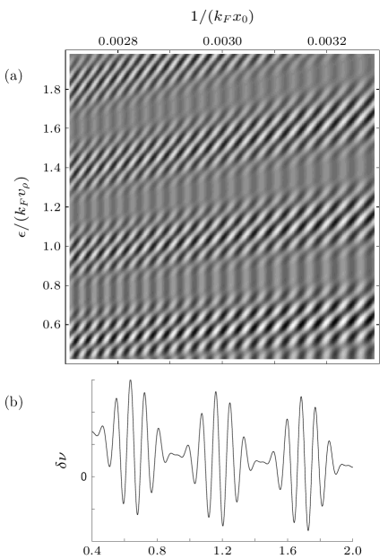
Figure 1: The oscillatory part of the density of states, see Eqs. (Signatures of spin-charge separation in scanning probe microscopy)–(Signatures of spin-charge separation in scanning probe microscopy), in arbitrary units. The parameters used are $g=0.8$ and $v_{\rho}/v_{\sigma}=1.4$. (a) Density plot as a function of $\epsilon$ and $1/x_{0}$. The main feature of the moiré pattern, i.e., fast oscillations appearing as slanted bright and dark regions with a slowly modulating amplitude, is captured by Eq. (Signatures of spin-charge separation in scanning probe microscopy). The contribution of Eq. (Signatures of spin-charge separation in scanning probe microscopy) appears as fainter vertical lines in the regions where the amplitude of the main oscillations is small. (b) Energy dependence at $k_{F}x_{0}=300$.

To illustrate these ideas further, we plot $\delta\nu$ in Fig. 1, using $g=0.8$ and $v_{\rho}/v_{\sigma}=1.4$. This choice of parameters corresponds to a relatively weak interaction, for which the assumptions leading to Eq. (Signatures of spin-charge separation in scanning probe microscopy) are valid (with these parameters, $C_{\sigma\sigma}=0.959$ and $C_{\rho\sigma}=0.964$). The moiré pattern expressed by Eq. (Signatures of spin-charge separation in scanning probe microscopy) is clearly visible in Fig. 1(a). This pattern may then be used to obtain the spin and charge mode velocities.

A measurement of $\nu(\epsilon)$ may probe spin-charge separation even in an experiment with a fixed (and maybe unknown) value of $x_{0}$. Indeed, Eq. (Signatures of spin-charge separation in scanning probe microscopy) shows that the number of fast oscillations of $\delta\nu_{1}(\epsilon)$ fitting between two adjacent minima of the slow amplitude modulation is $(v_{\rho}+v_{\sigma})/(v_{\rho}-v_{\sigma})$. For example, in Fig. 1(b) there are 6 such oscillations, corresponding to $v_{\rho}/v_{\sigma}=1.4$.

The SPM method considered here has connections with the STM technique studied in Refs. eggert1 ; eggert2 ; kivelson . The differences between the two methods arise from the different role of the scanning tip: In STM it is used to measure the local density of states rather than for creating a scattering potential for the electrons. In both cases, the measured differential conductivity exhibits oscillations as a function of tip position, which contain information about the spin and charge velocities. The difference in setup, however, affects the details of these oscillations and their dependence on the Luttinger liquid parameters. In particular, the SPM setup does not give rise to long wavelength oscillations of the type predicted for STM eggert1 .

In conclusion, the theory presented in this Letter suggests a way to study spin-charge separation in a quantum wire by means of a scanning probe measurement. The clearest manifestation of the separation is in the beating pattern of the differential conductance as a function of applied bias, see Fig. 1. The SPM method may be experimentally useful as it only requires contacting a single wire at its ends, unlike STM or momentum conserving tunneling. Finally, we note that our results, obtained at $T=0$, also hold at finite temperature, provided the distance between the tunneling point and the position of the probe is shorter than the thermal length $v_{\sigma}/T$.

We thank Rafi de Picciotto, Shahal Ilani, and Amir Yacoby for useful discussions. This work was supported by NSF grants DMR-02-37296 and EIA-02-10736.

References

- (1)
- (2) F. D. M. Haldane, J. Phys. C: Solid State Phys. 14, 2585 (1981).
- (3) For a review see, e.g., M. P. A. Fisher and L. I. Glazman, in Mesoscopic Electron Transport, edited by L. L. Sohn, L. P. Kouwenhoven, and G. Schön (Kluwer Academic Publishers, Dordrecht, The Netherlands, 1997), p. 331.
- (4) M. Bockrath et al., Nature 397, 598 (1999).
- (5) Z. Yao, H. W. Ch. Postma, L. Balents, and C. Dekker, Nature 402, 273 (1999).
- (6) A. Altland, C. H. W. Barnes, F. W. J. Hekking, and A. J. Schofield, Phys. Rev. Lett. 83, 1203 (1999).
- (7) S. A. Grigera, A. J. Schofield, S. Rabello, and Q. Si, Phys. Rev. B 69, 245109 (2004).
- (8) O. M. Auslaender et al., Science 295, 825 (2002).
- (9) Y. Tserkovnyak, B. I. Halperin, O. M. Auslaender, and A. Yacoby, Phys. Rev. Lett. 89, 136805 (2002); Phys. Rev. B 68, 125312 (2003).
- (10) U. Zülicke and M. Governale, Phys. Rev. B 65, 205304 (2002).
- (11) D. Carpentier, C. Peça, and L. Balents, Phys. Rev. B 66, 153304 (2002).
- (12) S. Eggert, Phys. Rev. Lett. 84, 4413 (2000).
- (13) F. Anfuso and S. Eggert, Phys. Rev. B 68, 241301 (2003).
- (14) S. A. Kivelson et al., Rev. Mod. Phys. 75, 1201 (2003), Sec. III.
- (15) S. G. Lemay et al., Nature 412, 617 (2001).
- (16) M. A. Topinka et al., Science 289, 2323 (2000); M. A. Topinka et al., Nature 410, 183 (2001).
- (17) R. Crook et al., Phys. Rev. Lett. 91, 246803 (2003).
- (18) T. Ihn et al., Physica E 12, 691 (2002).
- (19) M. T. Woodside and P. L. McEuen, Science 296, 1098 (2002).
- (20) C. L. Kane and M. P. A. Fisher, Phys. Rev. Lett. 68, 1220 (1992).
- (21) See D. G. Polyakov and I. V. Gornyi, Phys. Rev. B 68, 035421 (2003), and references therein.
- (22) R. Egger and H. Grabert, Phys. Rev. Lett. 75, 3505 (1995).