POWER-LAW SPIN CORRELATIONS IN PYROCHLORE ANTIFERROMAGNETS

Abstract

The ground state ensemble of the highly frustrated pyrochlore-lattice antiferromagnet can be mapped to a coarse-grained “polarization” field satisfying a zero-divergence condition From this it follows that the correlations of this field, as well as the actual spin correlations, decay with separation like a dipole-dipole interaction ($1/|R|^{3}$). Furthermore, a lattice version of the derivation gives an approximate formula for spin correlations, with several features that agree well with simulations and neutron-diffraction measurements of diffuse scattering, in particular the pinch-point (pseudo-dipolar) singularities at reciprocal lattice vectors. This system is compared to others in which constraints also imply diffraction singularities, and other possible applications of the coarse-grained polarization are discussed.

I introduction

Highly frustrated antiferromagnets are characterized by a very large number of essentially degenerate states, such that in a range of temperatures much smaller than the spin interaction scale they have strong local correlations, yet fail to order ramirez : diffuse scattering is the obvious probe of such a state. In this paper, I make the point that the classical ground-state ensemble can entail constraints that ensure a generic power-law decay of correlations: a picture of theses state as “liquid-like” (i.e. featureless) is thus imcomplete.

We consider specifically the pyrochlore lattice, consisting of corner-sharing tetrahedra, partly because of its simplicity as a model [high (cubic) symmetry and nearest-neighbor interactions], but most importantly because it is the magnetic lattice in many real systems: the B-site spinels lee00 ; lee02 , two families of pyrochlores represented by $\rm CsNiCrF_{6}$ harris94 ; harris97a , and the oxides $\rm Y_{2}Mn_{2}O_{7}$ Y2Mo2O7 , and even the transition-metal lattice in “frustrated itinerant” antiferro- or ferrimagnetic Laves phases, such as $\rm Y_{1-x}Sc_{x}Mn_{2}$ shi93 ; ballou . Ferroelectric degrees of freedom (water ice bernal-pauling ; youngblood ) and charge order (in magnetite an56 ) are also equivalent to pyrochlore systems.

Different pyrochlores show a wide variety of magnetic behaviors at low temperatures: apart from long-range order, these include lattice distortions lee00 ; tcherny , “spin-ice” behavior harris97b ; ramirez-spinice ; Si99 ; Bra01a ; Bra01b , paramagnetism (in $\rm Tb_{2}Ti_{2}O_{7}$) down to low temperatures, Tb2Ti2O7 or spin glass freezing (in $\rm Y_{2}Mo_{2}O_{7}$ even when structural disorder is quite small Y2Mo2O7 . However, most of these have a cooperative paramagnet regime at higher temperatures – but still quite low compared to the interaction scale $J$ – demonstrating that they have a large set of nearly degenerate (and accessible) states. The present paper addresses this phase, as it would be extrapolated to zero temperature.

In the remainder of this section, I review the lattice and the ground states of a pyrochlore antiferromagnet, and survey three situations in which it can be modeled by the ensembles used in this paper. Then (Sec. II the mapping of the low-temperature states of the Ising model to the “diamond ice” model is to construct a coarse-grained polarization field, which functions somewhat like an order parameter for this model, and this is used to predict some unusual features of the magnetic diffuse scattering. Sec. III presents another version of the derivation, which not only gets the long-wavelength behavior (corresponding to the neighborhoods of special points in the Brillouin zone) but provides an approximation for the entire zone. I also discuss (Sec. IV) other situations in which local constraints in a ground state produce diffraction singularities, and speculate on other questions that can be addressed using the insight that the polarization field contains the important long-wavelength degrees of freedom.

A parallel paper moessner-dipolar contains many of the same results.

I.1 Pyrochlore lattice and Hamiltonian

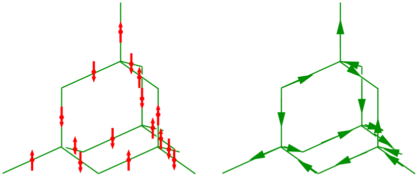
Figure 1: (a) Ising ground state on fragment of pyrochlore lattice; spins are shown on edges of a diamond lattice. (b). The corrsponding ice-model arrows between the diamond vertices.

The pyrochlore lattice consists of corner-sharing tetrahedra arranged in cubic (fcc) symmetry. Its key property is that the sites are the bond midpoints of a diamond lattice. [See Fig. 1; other figures emphasizing the tetrahedra are in Refs. tcherny, or moessner98a, ; moessner98b, .] For future use, we define vectors pointing towards the four corners of a tetrahedron,

$$\ {\bf u}_{1,2,3}\equiv[{\textstyle{1\over 4}},-{\textstyle{1\over 4}},-{\textstyle{1\over 4}}]\quad$$

$${\bf u}_{4}\equiv[{\textstyle{1\over 4}},{\textstyle{1\over 4}},{\textstyle{1\over 4}}]\qquad+\text{cyclic perms}.$$ (1)

In the diamond lattice, every even-to-odd bond vector is a ${\bf u}_{m}$.

The basic results derived in this paper are transferable to other lattices in which the spins sit on the bonds of a bipartite lattice, and with antiferromagnetic interactions among all spins on bonds sharing a common endpoint,such that their sum is constrained to a fixed value. Besides the pyrochlore lattice, this class includes the kagomé lattice, the two-dimensional “checkerboard” lattice, moessner98a ; moessner98b , the “sandwich” lattice modeling SCGO and consisting of two kagomé layers linked by an additional triangular layer of spins, broholm-SCGO ; henley-HFM00 ; kawamura and the garnet lattice petrenko .

The spin Hamiltonian, having only nearest-neighbor antiferromagnetic exchange, can be cast as a sum of squares:

$${\cal H}_{\rm spin}={J_{\rm spin}}\sum_{\langle ij\rangle}{\bf s}_{i}\cdot{\bf s}_{j}+{\rm const}=\frac{{J_{\rm spin}}}{2}\sum_{\alpha}{\bf L}_{\alpha}^{2},$$ (2)

where the total spin of four sites in a tetrahedron is

$${\bf L}_{\alpha}\equiv\sum_{i\in\alpha}{\bf s}_{i}$$ (3)

where $\alpha$ labels each diamond site and “$i\in\alpha$” runs over the surrounding four spins. For simplicity, I will mostly treat the case with Ising spins $t_{i}$. (There is little loss of generality, in view of Sec. I.2, below.)

$${\cal H}={\textstyle{1\over 2}}J\sum_{\alpha}L_{\alpha}^{2}=J\sum_{\langle ij\rangle}t_{i}t_{j}+{\rm const}.$$ (4)

From (4) it is evident that any state with

$$L_{\alpha}=0.$$ (5)

is a classical ground state; these are massively degenerate. The frustration of the pyrochlore Ising model, and the extensive ground state entropy implied by (5), were recognized very early an56 .

I.2 Temperature regimes and validity of Ising model

Here I discuss the three different situations in which realistic models can be treated under this paper’s scheme. [Readers who are content with a treatment of an Ising toy model, and do not immediately demand any connection to experiment, may skip to Sec. II where the central result is derived.]

First, it is possible that spin anisotropies (additional to (2)) reduce the ground state manifold to the Ising states. If the lattice is to remain cubic, the preferred axis cannot be the same for each spin, but instead is $\hat{\bf u}_{m(i)}$, where $\hat{\bf u}_{m}=4{\bf u}_{m}/\sqrt{3}$ is the unit vector of (1), and $m(i)$ labels the direction of the diamond-lattice bond on which spin $i$ sits. Assuming the spins are strongly aligned, one puts ${\bf s}_{i}=t_{i}\hat{\bf u}_{m(i)}$ and the Hamiltonian reduces to (4) with $J=-{J_{\rm spin}}/3$, since $\hat{\bf u}_{m}\cdot\hat{\bf u}_{m^{\prime}}=-1/3$ for $m\neq m^{\prime}$, and $m(i)\neq m(j)$ for nearest neighbors. This is the “spin-ice” model harris97b ; ramirez-spinice .

The other two situations correspond to isotropic Heisenberg models in the large-$S$ semiclassical regime (where $S$ is the spin length). This is necessary to guarantee that (5) is a good starting point for specifying the ground states. One can identify a succession of energy scales in the pure nearest-neighbor Heisenberg antiferromagnet, corresonding to successive breakings of the grond state degeneracy as more effects are considered.

The largest scale is $E_{J}\sim zJS^{2}$ where $z$ is the coordination number; this is the scale of the mean-field (classcial) part of the exchange energy, and of the Curie-Weiss constant. At temperatures $T\ll E_{J}$, it is reasonable to approximate the spin ensemble by a subset of the ground-state ensemble.

The spin-wave spectrum $\{\omega_{j}\}$ depends upon which state we linearized around. Thus, the total spin-wave zero-point energy (to harmonic order, $\sum_{j}{\textstyle{1\over 2}}\hbar\omega_{j}$) partially breaks the ground-state degeneracy, favoring collinear states,  shen82 ; hen89 . This is expressed quantitatively by an effective Hamiltonian oja ; larhen90 ; henley-HFM00 , with coupling constant $\sim E_{\rm coll}$, where the next largest scale is $E_{\rm coll}\sim JS\ll E_{J}$. (Even when $S$ is not so large, e.g. $S=5/2$ as with real spins, the coefficient of $JS$ is commonly less than $1/10$ so the inequality is valid.) In lattices other than pyrochlore, one finds a similar regime in which a discrete subset of the classical ground states (e.g. coplanar states, ritchey ; chubukov in the kagomé case) gets selected by the harmonic zero-point energy.

Finer treatment of the spin-wave fluctuations produces an even smaller energy scale $E_{\rm disc}$ for selection among the discrete states. In the kagomé case, chubukov ; chan ; this is due to anharmonic terms in the Holstein-Primakoff expansion, so that $E_{\rm disc}\propto S^{2/3}\ll S$. In the pyrochlore case, besides the anharmonic terms, $E_{\rm disc}$ does include contributions of $O(JS)$ from the harmonic terms. pyro-Heff . However, these terms only partly break the degeneracy, and the coefficients are small, so we can still assume $E_{\rm disc}\ll E_{\rm coll}$.

Thus, the second regime in which the Ising theory models the correlations is $E_{\rm disc}<T<E_{\rm coll}$. One expects a symmetry breaking to long-range collinear order, in which a global axis ${\hat{\bf n}}$ is spontaneously adopted and each spin is given by ${\bf s}_{i}=t_{i}{\hat{\bf n}}$, with $t_{i}=\pm 1$, plus small fluctuations. This phase is a kind of “spin nematic” chancole91 . The energy terms distinguishing different Ising states are unimportant since $T>E_{\rm disc}$, hence the spin ensemble is roughly the ground states of (4), as claimed.

Of course, in the real world there is another energy scale $E_{\rm pert}$ for perturbations of the pure Heisenberg Hamiltonian, representing the magnitude further-neighbor exchange and dipole couplings, as well as lattice distortions, and disorder, which cause a transition or freezing into some other state at sufficiently low temperature, so the regime of the spin nematic-like phase is really ${\rm max}(E_{\rm disc},E_{\rm pert})<T<E_{\rm coll}$.

Finally, the third situation is when $E_{\rm coll}\ll T\ll E_{J}$. This ensemble is well modeled by the low-$T$ limit of the classical Heisenberg model. It turns out (Sec. II.4, below) that the key notion of “polarization” does extend to the Heisenberg spin case. I have mostly neglected that case in this paper because, at my level of approximation, the results look identical; it would merely obscure the notation by adding spin-component indices everywhere.

II Coarse-graining, Fourier mode fluctuations, and long-range correlations

In this section, I present the steps leading to power-law correlations using the framework of a continuum theory, in the ideas appear more transparently.

II.1 Ice mapping and local polarization

In fact the pyrochlore (Ising) ground states map 1-to-1 onto those of the well-known diamond-lattice ice model an56 ; liebmann86 , in which the degrees of freedom are arrows along the lattice bonds. In the map, every tetrahedron center becomes a vertex of the diamond lattice, while the spin sites map to bond centers of the diamond lattice. Each spin $t_{i}=+1(-1)$ maps to an arrow pointing along the corresponding diamond lattice edge, in the positive (negative) sense from the even to the odd vertex. This well-known mapping  an56 ; liebmann86 ; Hen92 is also used to model the “spin ice” system Dy₂Ti₂O₇ (and also Ho₂Ti₂O₇), wherein local $\langle 111\rangle$ anisotropy plus ferromagnetism makes a highly frustrated Ising model harris97b ; ramirez-spinice ; Si99 ; Bra01a .) The ground state condition – net spin of every tetrahedron is zero – maps to the “ice rule” the numbers of incoming and outgoing arrows are equal at every vertex  bernal-pauling .

The key object in this paper is the ice polarization field. On a diamond-lattice bond a polarization $t_{i}{\bf u}_{m(i)}$ can be defined, aligned from the even to odd diamond-lattice vertex if the spin is up, oppositely if it is down; here $m(i)$ is the local 3-fold axis of site $i$. On every diamond vertex, we define the mean of this polarization over the surrounding tetrahedron of spins:

$${\bf P}({\bf R}_{\alpha})\equiv\sum_{i\in\alpha}t_{i}{\bf u}_{m(i)}.$$ (6)

The six possible ground-state configurations of that tetrahedron correspond to ${\bf P}({\bf R}_{\alpha})=(\pm 1,0,0)$, $(0,\pm 1,0),$ or $(0,0,\pm 1)$.

Finally, the coarse-grained arrow field ${\bf P}({\bf r})$ is the coarse-grained polarization averaged over some larger neighborhood and assumed to vary smoothly.

II.2 Effective free energy and correlations

The ground-state entropy density is a function of the average polarization. A subensemble of states in which ${\bf P}$ is large (which can be forced by boundary conditions) has relatively little freedom for rearrangements of the spins or arrows; indeed, for a saturated polarization such as ${\bf P}=(1,0,0)$ the ensemble consists of a single microstate. Thus it is very plausible that the entropy density has a maximum for zero polarization. Therefore, to lowest order, the total free energy (arising entirely from entropy), as a function of coarse-grained ${\bf P}({\bf r})$, has the form

$$F_{\rm tot}(\{{\bf P}({\bf r})\})/T=v_{\rm cell}^{-1}\int d^{3}{\bf r}{\textstyle{1\over 2}}\kappa|{\bf P}({\bf r})|^{2},$$ (7)

where $v_{\rm cell}=a^{3}/4$ is the volume of a primitive unit cell. The “stiffness” $\kappa$ is dimensionless, as appropriate since it is purely entropic in origin.

Corresponding to the condition (5), i.e. the ice rule, ${\bf P}({\bf r})$ satisfies a divergence constraint

$$\nabla\cdot{\bf P}({\bf r})=0$$ (8)

like a magnetic field without monopoles. Eqs. (7) and (8) look, respectively, like the field energy of a magnetic (or electric) field, and its divergence constraint, in the absence of monopoles (or charges). These equations, together, signify that that the probability distribution of the (long-wavelength portion of) the polarization field is the (constrained) Gaussian distribution

$${\rm Prob}(\{{\bf P}({\bf r})\})\propto e^{-F(\{{\bf P}({\bf r})\})/T}\prod_{\bf r}\delta(\nabla\cdot{\bf P}({\bf r}))$$ (9)

Fourier transforming (7) simply gives $F_{\rm tot}=\sum_{\bf k}{\textstyle{1\over 2}}\kappa|{\bf P}({\bf k})|^{2}$, so a naive use of equipartition would give $\langle P_{\mu}(-{\bf k})P_{\nu}({\bf k})\rangle=(1/{\kappa})\delta_{\mu\nu}$. But the divergence constraint (8) imposes

$${\bf k}\cdot{\bf P}({\bf k})=0$$ (10)

in Fourier space. Thus the correct result has the longitudinal fluctuations projected out:

$$\langle P_{\mu}(-{\bf k})P_{\nu}({\bf k})\rangle=\frac{1}{\kappa}\Bigl{(}\delta_{\mu\nu}-\frac{k_{\mu}k_{\nu}}{|{\bf k}|^{2}}\Bigr{)},$$ (11)

Fourier transforming (11) back to direct space gives

$$\langle P_{\mu}(0)P_{\nu}({\bf r})\rangle\cong\frac{4\pi}{\kappa}\Bigl{[}\delta({\bf r})+\frac{1}{r^{3}}(\delta_{\mu\nu}-3\hat{r}_{\mu}\hat{r}_{\nu})\Bigr{]}$$ (12)

at large separations ${\bf r}$ (where $\hat{\bf r}\equiv{\bf r}/|{\bf r}|.$) Correlations have the spatial dependence of a dipole-dipole interaction, which is a power law. Models that exhibit such correlations – including the pyrochlore system, so often described as “liquid-like”, – are thus, in a sense, in a critical state. [The generalization of (12) for $d$-dimensional real space. would be a $1/r^{d}$ decay.]

This criticality was first appreciated in the ice model itself, being detected originally in a simulation stillinger . A functional form with a dipolar singularity like (11) was produced by a clever random-walk approximation to a series expansion villain . The universal explanation, made here, that dipolar correlations arise from (7) with the divergence condition, was first put forward to explain experiments on two-dimensional ice-like systems youngblood .

Ref. huse-dimer, have also presented an ansatz equivalent to (9), derived the dipolar correlations, and confirmed them by simulations, for the dimer covering of a simple cubic lattice. [See their eq. (3).] The $1/|{\bf r}|^{3}$ decay has also been obtained analytically and numerically in Ref. hermele, , for the pyrochlore model of this present paper.

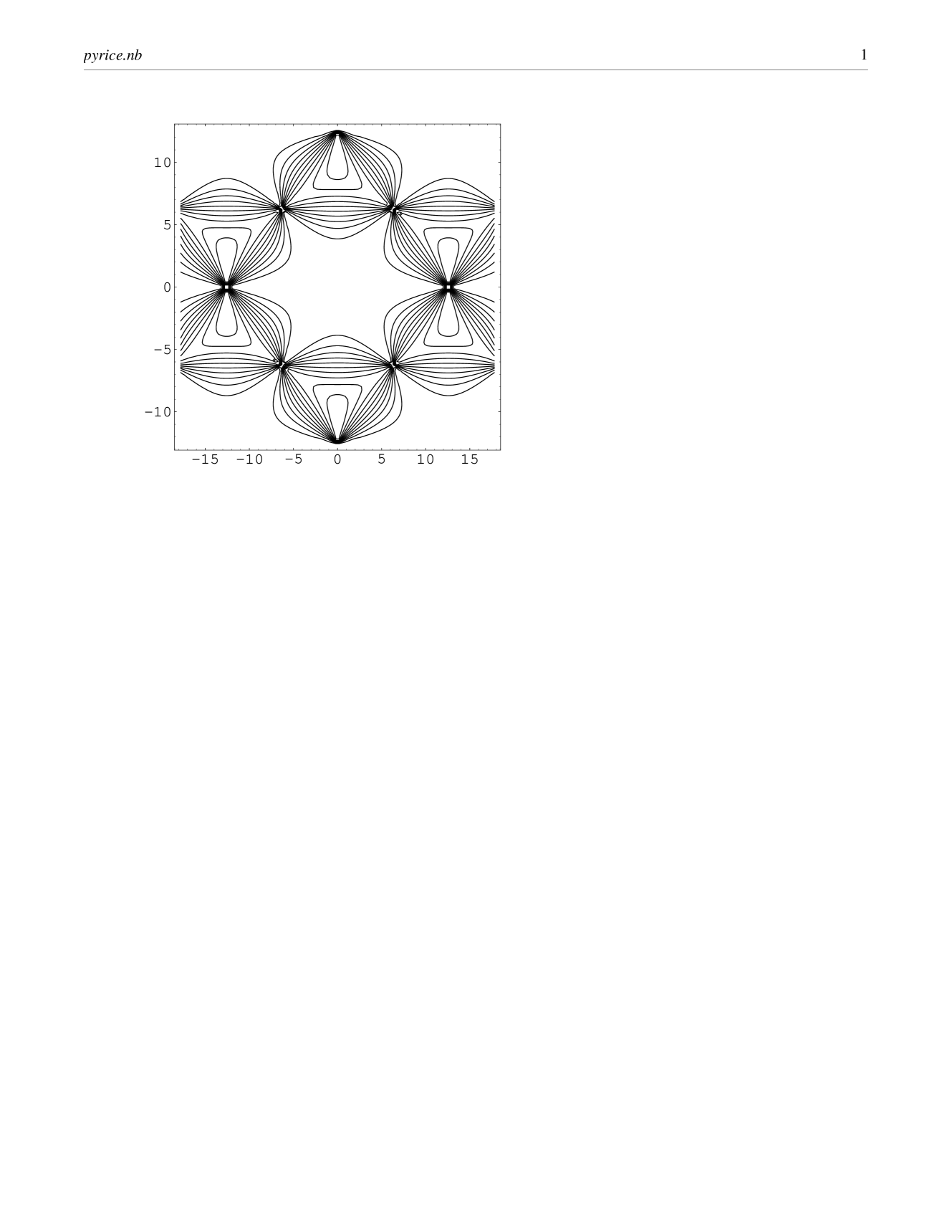
Figure 2: Calculated structure factor in the plane normal to $[1\bar{1}0]$. (The figure is the same slice as shown in Refs. zinhar95, and harris95, .)

Ref. moessner98b, , Sec. II D 1, recognized that the ground-state constraint in the Heisenberg pyrochlore antiferromagnet (5) entails long-range correlations, but in the absence of the polarization concept, the argument’s form is diffuse, and it was not possible to predict an explicit functional form. An interesting heuristic argument was made there to justify the empirical fact of the “bowtie” shape (see Fig. 2) taken by the diffuse scattering: in other words, that it takes a scaling form in terms of $q_{x}/q_{\perp}$.

II.3 Diffraction consequences

II.3.1 Spin structure factor

There is a linear relationship between the actual Ising spins and the ice arrows: specifically, the map (6), from spins to the the diamond-vertex polarization is actually invertible:

$$t({\bf R}\pm{\textstyle{1\over 2}}{\bf u}_{m})=4{\bf u}_{m}\cdot{\bf P}({\bf R}),$$ (13)

where we take the $+$ or $-$ signs for even and odd vertices ${\bf R}$, respectively. Thus it is not surprising that the pseudodipolar correlations (12) of the latter imply similar $1/r^{3}$ correlations for the former. However, the coefficients relating these (namely, the $\{{\bf u}_{m}\}$ vectors) are staggered in sign.

To see this, first Fourier transform (13), using the fact that

$${\bf u}_{m,x}={\textstyle{1\over 4}}e^{{\textstyle{1\over 2}}i{\bf K}_{200}\cdot({\bf u}_{m}-{\bf u}_{4})},$$ (14)

similarly $uu_{m,y}$ with ${\bf K}_{020}$, etc. When this is inserted into the formula for ${\tilde{t}}({\bf k})$ [similar to (23)], the staggering contained in the ${\bf u}_{m}$ factors shifts the argument by the reciprocal space vector ${\bf K}_{200}$ so that ${\tilde{t}}({\bf K}_{200}+{\bf q})\propto P_{x}({\bf q})$, etc. Consequently, the singularities of the spin structure factor in reciprocal space are pseudo-dipolar in form, just like (15), but occur at nonzero reciprocal lattice vectors ${\bf K}$ rather than at ${\bf q}=0$.

Let ${\tilde{t}}({\bf k})$ be the Fourier transform of the spins. The structure factor (i.e. the neutron diffraction intensity. modulo polarization factors) has pseudo-dipolar singularities

$${\langle|{\tilde{t}}({\bf K}_{200}+{\bf q})|^{2}\rangle}\propto\frac{q_{\perp}^{2}}{q_{\parallel}^{2}+q_{\perp}^{2}}$$ (15)

Here ${\bf K}_{200}\equiv[2\pi/a](2,0,0)$ is a reciprocal lattice vector; and ${\bf q}_{\parallel}\equiv q_{x}$ and $q_{\perp}^{2}\equiv q_{y}^{2}+q_{z}^{2}$. Near ${\bf K}_{111}\equiv 2\pi(1,1,1)$, the same form holds with ${\bf q}_{\parallel}$ and ${\bf q}_{\perp}$ being the components of ${\bf q}$ parallel and perpendicular to the $(111)$ direction.

The elastic constant $\kappa$ must be determined from Monte Carlo simulations. Yet, without knowing it, we can still make the nontrivial prediction that the diffuse scattering has quantitative the same strength near ${\bf K}_{111}$ as it does near ${\bf K}_{200}$. In an isotropic Heisenberg model, these pseudodipolar singularities can be distinguished from true dipolar singularities in neutron scattering experiments, since they are independent of spin direction. They can be seen in only one spatial direction around each reciprocal lattice point.

The functional form (15) has nodes which we expect (correctly) are a consequence of symmetry and therefore extend throughout reciprocal space, beyond the small-${\bf q}$ limit in which (15) was derived. For example, (15) indicates that

$${\langle|{\tilde{t}}(k_{x},0,0)|^{2}\rangle}\equiv 0$$ (16)

for wavevectors anywhere along the entire (100) axis. Similarly the structure factor is zero along the (111) axis near ${\bf K}_{111}$ from (15) Since ${\bf k}=(000)$ is the intersection of seven distinct axes, along each of which the structure factor must vanish, we deduce that the diffuse scattering vanishes near the origin as

$$\langle|t({\bf k})|^{2}\rangle\propto(k_{x}^{2}k_{y}^{4}+{\text{5 permutations}})-6k_{x}^{2}k_{y}^{2}k_{z}^{2}.$$ (17)

Indeed, experiments and all simulations on pyrochlore antiferromagnets find quite small diffraction throughout the first Brillouin zone.

II.3.2 Derivation of nodal lines

It is possible to confirm (16) without using coarse-graining, by sharpening an argument made in Sec. II D of Ref. moessner98b, . (I have written the steps in detail, so it will be clear whether they do or do not carry through for other lattices.)

Partition the pyrochlore lattice sites into (100) planes labeled by $x$, and define ${t_{\rm plane}}(x)\equiv\sum_{x_{i}=x}t_{i}$. Then consider, for example, the tetrahedra with centers at $x=0$: each such tetrahedron includes a pair of spins with $x_{i}=-{\textstyle{1\over 4}}$ and another pair with $x_{i}=+{\textstyle{1\over 4}}$. By the ground-state constraint (5) the sum of one pair is the negative of the sum of the other pair. Since every spin with $x_{i}=\pm{\textstyle{1\over 4}}$ belongs to exactly one such tetrahedron, this implies ${t_{\rm plane}}(-{\textstyle{1\over 4}})=-{t_{\rm plane}}({\textstyle{1\over 4}})$; and by Bravais lattice periodicity, ${t_{\rm plane}}({\textstyle{1\over 4}}+{\textstyle{1\over 2}}n)=(-1)^{2}{t_{\rm plane}}({\textstyle{1\over 4}})$. Since all spins have $x_{i}={\textstyle{1\over 4}}+{\textstyle{1\over 2}}n$ for some $n$,

$${\tilde{t}}(k_{x},0,0)\propto\sum_{n}e^{-ik_{x}({\textstyle{1\over 4}}+{\textstyle{1\over 2}}n)}(-1)^{n}{t_{\rm plane}}({\textstyle{1\over 4}})$$ (18)

which cancels, except for a possible Bragg peak when $k_{x}$ is a multiple of $2\pi$. However, in the maximum entropy state that we assumed in Sec. II.2, the average spin in one of these planes – which is proportional to the mean polarization $P_{x}$ – is zero, so ${\tilde{t}}(k_{x},0,0)=0$ for all $k_{x}$.

A similar, but more complicated, argument works for a $\{111\}$ direction. Let $\xi_{i}\equiv{\bf r}_{i}\cdot\frac{1}{\sqrt{3}}(1,1,1)$ be the projection of site $i$ on the $(111)$ axis, and redefine ${t_{\rm plane}}(\xi)$ as the spin sum over the spin plane with $\xi_{i}=\xi$. Each tetrahedron with $\xi=0$ includes three spins in the $\xi=-1/4\sqrt{3}$ plane and one spin in the $\xi=\sqrt{3}/4$ plane, and every spin in either plane belongs to a unique tetrahedron; consequently ${t_{\rm plane}}(-1/4\sqrt{3})=-{t_{\rm plane}}(+\sqrt{3}/4)$, even though one plane has three times as many spins as the other. Furthermore these unequal planes are equally spaced, so ${t_{\rm plane}}(\sqrt{3}/4+n/\sqrt{3})=(-1)^{n}{t_{\rm plane}}(\sqrt{3}/4)$ and the rest of the argument follows as before.

II.3.3 Alternate derivation of nodal lines

There is an alternate way to see that diffuse intensity must be small near the zone center. Let ${\bf P}^{+}({\bf k})$ be Fourier transform of the discrete polarization on (say) even diamond sites, defined like (24). On the one hand, the Fourier transform of the constraint (5) at odd vertices

$$4{\bf G}(-{\bf k})\cdot{\bf P}({\bf k})=0$$ (19)

where

$${\bf G}({\bf k})=\sum_{m=1}^{4}e^{i{\bf k}\cdot{\bf u}_{m}}{\bf u}_{m}\approx{\textstyle{1\over 4}}i{\bf k}$$ (20)

at small wavevectors. On the other hand, we can start from (13) and take its Fourier transform – this time, not taking advantage of (14); the result is

$${\tilde{t}}({\bf k})=4{\bf G}({\textstyle{1\over 2}}{\bf k})\cdot{\tilde{{\bf P}}}({\bf k}).$$ (21)

Near ${\bf k}=0$, comparing (21) and (19) and recalling that ${\bf G}(-{\textstyle{1\over 2}}{\bf k})\approx-{\textstyle{1\over 2}}{\bf G}({\bf k})$, we conclude that ${\tilde{t}}({\bf k})\approx 0$, as I asserted earlier. Furthermore, whenever ${\bf k}$ is along a $\{100\}$ or a $\{111\}$ symmetry axis, ${\bf G}({\bf k})$ is parallel to that same axis by symmetry (for all ${\bf k}$), hence structure factor (16) is null all along those axes.

II.4 Generalization to Heisenberg spins

In the case of isotropic $n=3$ component spins, we can reiterate all the coarse-graining arguments of Sec. II in terms of the Heisenberg spin components. Polarization components are defined as in (6) but now for each Cartesian spin component, so the polarization field is now a tensor carrying not only space but also spin indices: $({\bf P}_{\alpha})_{\beta\mu}\equiv\sum_{i\in\alpha}({\bf s}_{i})_{\beta}({\bf u}_{m(i)})_{\mu}$. As in the Ising case, it is easy to convince oneself that the entropy density is maximum when ${\bf P}=0$. Hence we expect that (7) remains valid, except that each $|{\bf P}({\bf r})|^{2}$ is now interpreted as a tensor norm (sum of squares of all tensor elements). Finally, (8) now becomes three equations, one for each spin-space component.

The basis of this paper – and the signatures implied in the diffuse diffraction – extends even to Heisenberg pyrochlore antiferromagnets in a magnetic field ${\bf H}$. The replacement ${\cal H}\to{\cal H}-{\bf H}\cdot\sum_{i}{\bf s}_{i}$ is equivalent to substituting

$${\bf L}_{\alpha}\to{\bf L}_{\alpha}-{\bf H}/2{J_{\rm spin}}$$ (22)

in (4). In the case of vector spins (but not Ising spins!), one achieves a ground state by satisfying ${\bf L}_{\alpha}={\bf H}/2{J_{\rm spin}}$ on every tetrahedron. Simply replacing $\delta{\bf s}_{i}\equiv{\bf s}_{i}-{\bf H}/8$ in the definition of ${\bf P}({\bf r})$ (i.e subtracting off the mean spin expectation), provides a polarization appropriate to this ground state, which should exhibit the same sort of long-range correlations (but with an $|{\bf H}|$ dependence.)

III Lattice approximation

The continuum theory presented in Sec. II can only predict the shape of singularities at special points in reciprocal space. For a better comparison to experiments, a theory of the diffuse scattering throughout reciprocal space is desirable. Of course, whereas the result (12) is universal across a class of models as enumerated in Sec. II.1 and Sec. IV.3.1, the detailed shape of the scattering calculated here is specific to the pyrochlore lattice.

The derivation depends on lattice Fourier transforms. This unfortunately forces the introduction, for this section, a new indexing $t({\bf R}+{\textstyle{1\over 2}}{\bf u}_{m})$ and $L({\bf R})$ for the same objects $t_{i}$ and $L_{\alpha}$ defined previously, where ${\bf R}$ designate the diamond sites; the even sites ${\bf R}$ form an fcc Bravais lattice and we let $N$ be the number of primitive unit cells. Thus each pyrochlore site ${\bf r}_{i}$ is written ${\bf R}+{\textstyle{1\over 2}}{\bf u}_{m}$; the surrounding odd diamond vertices are at ${\bf R}+{\bf u}_{m}$.

$${\tilde{t}}_{m}({\bf k})=\frac{1}{\sqrt{N}}\sum_{\bf R}e^{-i{\bf k}\cdot({\bf R}+{\textstyle{1\over 2}}{\bf u}_{m})}t({\bf R}+{\textstyle{1\over 2}}{\bf u}_{m}).$$ (23)

The definition (3) is rewritten $L({\bf R})=\sum_{m=1}^{4}t({\bf R}\pm{\textstyle{1\over 2}}{\bf u}_{m}))$ taking $+$ and $-$ when ${\bf R}$ is an even or odd diamond vertex, respectively. Thus the Fourier transform of (3), restricted to even or odd vertices as indicated by the “$\pm$”, is

$$\tilde{L}^{\pm}({\bf k})=\frac{1}{\sqrt{N}}\sum_{m=1}^{4}e^{\pm{\textstyle{1\over 2}}i{\bf k}\cdot{\bf u}_{m}}{\tilde{t}}_{m}$$ (24)

III.1 Derivation of fluctuations

The simplest way to describe the approximation is first to imagine a distribution of spins

$${\rm Prob}(\{t_{i}\})\propto e^{-\sum_{i}\frac{t_{i}^{2}}{2t_{0}^{2}}}\exp(-{\beta_{\rm eff}}{\cal H}),$$ (25)

where ${\cal H}$ is given by (4), and ${\beta_{\rm eff}}$ ought to be the inverse temperature. The Gaussian factor in (26) may be viewed, in the Bayesian spirit of the maximum-likelihood approach, as a trivial a priori independent distribution before we account for any spin interaction. The second factor enforces spin correlations; here ${\cal H}(\{t_{i}\})$ is the Hamiltonian (4) for Ising spins, except that now $t_{i}$ is allowed to take any real value.

Adopting the limit ${\beta_{\rm eff}}\to\infty$, (25) reduces to

$${\rm Prob}(\{t_{i}\})\propto e^{-\sum_{i}\frac{t_{i}^{2}}{2t_{0}^{2}}}\prod_{\alpha}\delta(L_{\alpha})$$ (26)

The second factor in (26) imposes the ground state constraints (5) around every tetrahedron, both even and odd.

III.1.1 Ising spin correlations

Our goal is to evaluate $\langle t_{i}t_{j}\rangle$, and this is not hard to do using the Fourier transform (23). We must first rewrite $\prod_{\alpha}\delta(L_{\alpha})\propto\prod_{\bf k}\delta(L^{+}({\bf k}))\delta(L^{-}({\bf k}))$ in (26), and re-express this in terms of $\{{\tilde{t}}_{m}({\bf k})\}$.

Since different wavevectors decouple, it will be convenient to view ${\tilde{t}}_{m}({\bf k})$ as a complex 4-component vector. Then the even and odd vertex constraints take the form of orthogonality conditions:

$${\tilde{L}}^{\pm}({\bf k})\equiv\sum_{m=1}^{4}e^{\pm{\textstyle{1\over 2}}i{\bf k}\cdot{\bf u}_{m}}{\tilde{t}}_{m}({\bf k})\equiv(E^{\pm}({\bf k},{\tilde{t}}({\bf k}))=0$$ (27)

The coefficients are

$$E^{\pm}_{m}({\bf k})\equiv e^{\mp{\textstyle{1\over 2}}i{\bf k}\cdot{\bf u}_{m}}$$ (28)

so $E^{-}_{m}\equiv(E^{+}_{m})^{*}.$ The inner product is defined by

$$(A,B)\equiv\sum_{m=1}^{4}A_{m}^{*}B_{m}.$$ (29)

So, the distribution (26) can be rewritten in Fourier space as

$$\prod_{\bf k}\left[e^{-\frac{1}{2t_{0}^{2}}\sum_{m}^{4}|{\tilde{t}}_{m}({\bf k})|^{2}}\delta((E^{+}({\bf k}),{\tilde{t}})\delta((E^{-}({\bf k}),{\tilde{t}})\right].$$ (30)

Thus, for each ${\bf k}$ in (30), we now have a Gaussian distribution over a four-dimensional space, with two constraints reducing it to a two-dimensional subspace.

Our object is to obtain correlations of the form $\langle{\tilde{t}}_{l}(-{\bf k}){\tilde{t}}_{m}({\bf k})\rangle$. The result will essentiallly be the projector $\Pi$ into the subspace satisfying (27). If we define the $4\times 2$ matrix $E$, the columns of which are $E^{+}$ and $E^{-}$, then $4\times 4$ projection matrix for the (desired) space orthogonal to $E^{+}$ and $E^{-}$ is $\Pi\equiv I-E(E^{\dagger}E)^{-1}E^{\dagger}$. In fact

$$(E^{\dagger}E)=4\pmatrix{1&H\cr H^{*}&1},$$ (31)

$$(E^{\dagger}E)^{-1}=\frac{1}{4}(1-|H|^{2})^{-1}\pmatrix{1&-H^{*}\cr-H&1}$$ (32)

where the ${\bf k}$ argument in $E$ and $H$ was suppressed; here

$$H({\bf k})\equiv\frac{1}{4}\sum_{m}e^{i{\bf k}\cdot{\bf u}_{m}}=\cos\frac{k_{x}}{4}\cos\frac{k_{y}}{4}\cos\frac{k_{z}}{4}$$

$$-i\sin\frac{k_{x}}{4}\sin\frac{k_{y}}{4}\sin\frac{k_{z}}{4}.$$ (33)

[$H(-{\bf k})\equiv H({\bf k})^{*}$, $|H({\bf k})|^{2}=\frac{1}{4}(1+\cos\frac{k_{y}}{2}\cos\frac{k_{z}}{2}+\cos\frac{k_{x}}{2}\cos\frac{k_{z}}{2}+\cos\frac{k_{x}}{2}\cos\frac{k_{y}}{2})$. The final result is

$$\langle{\tilde{t}}_{l}(-{\bf k}){\tilde{t}}_{m}({\bf k})\rangle=t_{0}^{2}\left\{\delta_{lm}-[E(E^{\dagger}E)^{-1}E^{\dagger}]_{lm}\right\}$$ (34)

where $E$ and $(E^{\dagger}E)^{-1}$ are implicitly functions of ${\bf k}$ and are defined by (28) and (32).

Since ${\rm Tr}\Pi=2$, we must have $t_{0}^{2}=2$ to satisfy the normalization condition $\langle t_{i}^{2}\rangle=1$.

III.1.2 Spin structure factor

The structure factor, as measured in neutron diffraction, combines the four sublattice contributions. Write the Fourier transform of all the spins as ${\tilde{t}}({\bf k})\equiv\frac{1}{\sqrt{N}}\sum_{m}\sum_{\bf R}e^{-i{\bf k}\cdot({\bf R}+{\textstyle{1\over 2}}{\bf u}_{m})}t({\bf R}+{\textstyle{1\over 2}}{\bf u}_{m})=(M,\tilde{t}({\bf k}))$, where we used the 4-vector inner product and

$$M\equiv(1,1,1,1)$$ (35)

The structure factor is then a projection of (34) onto the $M$ vector, thus

$$\langle|{\tilde{t}}({\bf k})|^{2}\rangle=t_{0}^{2}M^{T}[I-E(E^{\dagger}E)^{-1}E^{\dagger}]M.$$ (36)

In the case of spin ice, the mapping of the Ising spins $\{t_{i}\}$ to the real spins is different (it is staggered). In this case, $M_{\beta m}=(\hat{{\bf u}}_{m})_{\beta}$. The pinch-point singularities will appear, but at different places (including the origin), because in this case the spins are the local polarizations. In this case, the scattering around the origin is no longer suppressed.

In either the antiferromagnet or the spin-ice case, there will be extinctions of the expected singularity at points where $(E^{\pm},M)$ happens to cancel.

Considering the form of (34), singularities in the spin fluctuations may (but do not necessarily) occur when the $2\times 2$ matrix $(E^{\dagger}E)$ is singular. In view of (32), this occurs when $|H({\bf k})|^{2}=1$. But that is precisely the defining condition for the fcc reciprocal lattice vectors ${\bf K}$. [This was derived by a different route in Sec. II.3.1.]

Indeed, $E^{+}({\bf K}_{200})=i(-1,-1,1,1)$ and $E^{+}({\bf K}_{111})=\frac{1+i}{\sqrt{2}}(-1,1,1,1)$. We see $E^{+}({\bf K})$ is proportional to a real four-vector. [That generically happens at a point in three-dimensional ${\bf k}$-space, since there are three independent phase relationships to be satisfied among the components $\{E^{+}_{m}\}$.] Then $E^{+}$ is proportional to $E^{-}$, and the rank of $E({\bf K})$ is reduced from two to one at these points, confirming that $E({\bf K})$ is singular.

The special lines in reciprocal space on which diffraction is zero, are those where the 4-vector of coefficients (35), relating the physical spin to the four sublattice spins ${\tilde{t}}_{m}({\bf k})$, happens to be orthogonal to both of the vectors in the null space of the $4\times 4$ matrix (34).

III.2 Finite temperature

In the approximations of Sec. II and Sec. III.1, where the tetrahedron constraint was imposed rigorously, we were forced to project out the corresponding fluctuation modes. It is possible to extend the approximation so as to permit small fluctuations of the tetrahedron magnetizations, as must be excited at $T>0$, starting from (25). Now, no projection is required, since a large coefficient ${\beta_{\rm eff}}$ tends to suppress those fluctuations, and so this ${\beta_{\rm eff}}<\infty$ case is actuallly more straightforward. [This subsection is essentially a streamlining of Ref. yoshida, , as converted to my notations.]

The Hamiltonian in (25) is a quadratic form in the $t_{i}$’s. Fourier transforming(4), and putting it into the 4-vector notation with (27), we get

$${\cal H}={\textstyle{1\over 2}}J\sum_{\bf k}\left[|L^{+}({\bf k})|^{2}+|L^{-}({\bf k})|^{2}\right]={\textstyle{1\over 2}}J({\tilde{t}},E^{\dagger}E{\tilde{t}}).$$ (37)

Thus, (25) becomes ${\rm Prob}(\{{\tilde{t}}_{m}\})\propto\exp(-{\textstyle{1\over 2}}({\tilde{t}},\lambda{\tilde{t}})$, where

$$\Lambda\equiv\frac{1}{t_{0}^{2}}I+{\beta_{\rm eff}}E^{\dagger}E.$$ (38)

and (34) gets replaced by

$$\langle t_{l}(-{\bf k})t_{m}({\bf k})\rangle=(\Lambda^{-1})_{lm}.$$ (39)

The matrix $E^{\dagger}E$ has rank two. It can be seen that, as ${\beta_{\rm eff}}\to\infty$, (39) indeed reduces to the projector (34).

The consequence of ${\beta_{\rm eff}}<\infty$ for correlations is that, in reciprocal space the pseudodipolar singularities (15), get rounded by the substitution

$${\bf q}^{2}\to{\bf q}^{2}+\xi^{-2}$$ (40)

in the denominator, where $\xi\sim{\beta_{\rm eff}}^{1/2}$ is a a correlation length. In real space, the power-law decays (12) acquire an $\exp(-r/\xi)$ factor that cuts them off, as noted in Ref. garanin, .

III.3 Other analytic approximations

Three prior treatments of the diffuse scattering in the pyrochlore arrived at a mathematical form more or less identical to (25), but with different formulas for the coefficients in these equations as a function if temperature. Thus, of course, their result is (39); however, they did not note the pseudodipolar (or, in the spin-ice case, literally dipolar) correlations which are implicit in these formulas at the $T=0$ limit.

The diffuse scattering problem was first addressed by Reimers reimers92b for Heisenberg, or in general $n$-component vector spins.) That derivation is based on mean field theory (Ornstein-Zernike correlations), which ought to be valid in the critical regime $T\to{T_{c}^{\rm MF}}$, where ${T_{c}^{\rm MF}}=J/n$. However, that is invalid in the pyrochlore case, since the real critical temperature is driven to zero. Even so, the ${\bf k}$ dependence of the result (eq. (15) of Ref. reimers92b, ), for the limit $T\to{T_{c}^{\rm MF}}$, is exactly of the form (25), with $1/t_{0}^{2}=3(T/{T_{c}^{\rm MF}}-1)$ and ${\beta_{\rm eff}}=1/T$.

Canals and Garanin garanin ; canals-garanin considered the classical pyrochlore antiferromagnet with $n$-component unit spins, in the large-$n$ limit which is tractable analytically. This is, in effect, like the “spherical model” approximation for finite-$n$, in that a constraint $|{\bf s}_{i}|=1$ on every spin is replaced by one on all $N$ spins, $\sum_{i}|{\bf s}_{i}|^{2}=N$. As they noted in Ref. garanin, , Sec. III, the $n=\infty$ limit is completely described by Gaussian approximations. Their result for small temperatures can be reduced to (25) with $1/t_{0}^{2}=n/3$ and ${\beta_{\rm eff}}=1/T$; this reduces to (26) as $T\to 0$.

Finally, Yoshida et al yoshida use an elaborate cluster-variational method to derive a sensible formula for the temperature-dependent diffuse scattering for the Ising ($n=1$) pyrochlore antiferromagnet (specifically, spin ice). Their result, taking the lowest-order finite temperature correction, amounts to (25) with $t_{0}^{2}=2$ and ${\beta_{\rm eff}}J=\frac{3}{16}e^{2J/T}$, which in the zero-temperature limit reduces to (26). [Note that $J_{\rm eff}/3$ of Ref. yoshida, is my $J$. My $E^{\pm m}$ are essentially linear combinations of the 4-vectors $c$ and $s$ of their eq. (B-3).]

Until now, I have only mentioned approximations which involve the connectivity of the sites and which can incorporate the long-range nature of the constraint. Some other approximations, intended mainly to model the bulk susceptibility, are based on a single isolated tetrahedron  harris95 ; moessner-berlinsky ; garcia-huber . Apart from the restriction that this tetrahedron has zero net spin, these approaches necessarily miss the long-range constraint and hence give a poor picture of the long-range correlations.

III.4 Comparison to diffraction in experiment and simulation

Several pyrochlore systems show the same characteristic diffuse scattering features: (i) the entire first Brillouin zone has a very low intensity (ii) intensity is zero along $\{100\}$ abd $\{111\}$ axes; (iii) there is a pinch-point singularity of form (15) at ${\bf K}_{200}$ and also ${\bf K}_{111}$ reciprocal lattice vectors. It should be noted that, since there are four spin sites per unit cell, the diffuse scattering is not periodic with the Brillouin zone.

Experimentally, such features were seen in an itinerant Laves phase (Ref. ballou, , Fig. 3); in the pyrochlore CsNiCrF₆” (Ref. harris97a, , Fig. 4); and most recently in the spinel ZnCrO₄ (Ref. lee02, , Fig. 3(a,b)), in the higher-temperature regime above a structural transition. In simulations, such patterns appeared in Fig. 2 of Ref. zinhar95, , Fig. 4 of  Ref. harris97a, , and in Ref. moessner98b, . For comparison, spin-1/2 results from exact diaagonalization are shown in Ref. canals98, , Fig. 4; they are qualitatively similar, but less sharp.

Images of analytic large-$n$ calculations of Garanin and Canals can also be compared: Ref. canals-garanin, , Fig. 4 (which is the kagomé system) and Ref. Can00, , Fig. 6.

Ref. moessner-kagice, , in their Fig. 5, plot diffuse scattering from simulation of a two-dimensional spin problem equivalent to the honeycomb dimer covering. (This is a plane of spins in the “kagomé -ice” phase, whereby an external field applied to a “spin-ice” pyrochlore system causes $\{111\}$ planes to decouple). The pinch-points (called “bowties” by those authors) are prominently visible, which are diagnostic of pseudodipolar correlations on real space.

The structure factor (15) has a local maximum at $q+x=0$, if we vary $q_{x}$ along a line ${\bf q}_{\perp}={\rm const}$, offset slightly from the $q_{x}$-axis. The same behavior is found around ${\bf K}_{111}$ and, of course, all other symmery-equivalent reciprocal lattice vectors: the structure factor has maxima in the plane perpendicular to the radial direction in reciprocal space. The union of these planar facets forms the same shape (a cuboctahedron) as the boundary of the FCC lattice’s first Brillouin boundary, but doubled in all three directions. Indeed, in a plane of reciprocal space from a single crystal of Y_1-xSc_xMn₂, the diffuse scattering is concentrated near the lines where this plane cuts the Brillouin zone faces ballou .

Powder diffraction data from pyrochlores showed a characteristic maximum  reimers92b which was seen experimentally harris94 , and in simulation reimers92a . This is consistent with the fact that the (doubled) Brillouin zone boundary (where diffraction is maximum along any ray in reciprocal space) is roughly a sphere. (Note that powder averaging, in the vicinity of ${\bf K}_{200}$, amounts to integrating (15) over $q_{y}$ and $q_{z}$, which yields a weakly cusped function ${\rm Const}-2\pi q_{x}^{2}\ln q_{x}$.)

IV Discussion

In summary, it was found that a polarization can be defined in pyrochlore antiferromagnets which – in a ground state – exactly satisfies a divergence condition. The coarse-grained version of this is analogous to an order parameter, in being the natural variable to describe large-scale properties. The correlations were found (Sec. II) to have a pseudo-dipolar form which – since this is a pure power law – implies an infinite correlation length. These behaviors were repeated in a lattice-based derivation (Sec. III. In the rest of this section, I discuss other problems to which these findings or approaches could be extended or related.

IV.1 Implications for diffraction experiments

The argument of this paper suggests that the analytis of diffraction experiments ought to focus more on the characteristic features, such as pinch points, identified in Sec. II.3.1 and Sec. III.1.2. Deviations from the predictions at those places are sensitive measures of the extent to which the tetrahedron constraint is violated in the actual ensemble. Thus, it is suggested to analyze these experiments so as to extract the correlation length $\xi$, and to check how well the diffraction is suppressed along the predicted nodal lines. [A correlation length was extracted in Ref. zinhar95, from simulations, however in this case it was actually the finite size cutoff.]

Deviations in the overall pattern from the shape predicted in Sec. III.1.2 (which are consistent with simulations moessner-dipolar ) are likely to reflect additional terms in the Hamiltonian, as in Ref. lee02, .

Ref. lee02, have fitted the diffuse intensity as the Fourier transform, not of a single tetrahedron, but a single loop of 6 spins. However, contrary to the speculation in that paper, this does not necessarily indicate a physical state built from such hexagons. To explain this, I will outline an alternative, equally systematic way of fitting the diffuse diffraction data.

The constraint (4) implies a similar constraint on the matrix of correlation functions. Then one can express any valid correlation function using a basis of linearly independent, orthogonal functions in real space satisfying this constraint, in the spirit of e.g. spherical harmonics. The first of these terms is the same correlation that derives from the ring of six. The form observed lee02 is, from this viewpoint, the simplest possible shape, as one might expect at higher temperatures when all the other terms are damped out. To produce a pinch point, an infinite number of such functions would be needed, corresponding to a large spatial extent.

IV.2 Dynamics

It is well known that violations of the tetrahedron constraint (due to disorder, or thermal excitation) map to electric charges (in the language where ${\bf P}({\bf r})$ is an “electric field.” A defect in which three arrows point outwards has a “charge” of $Q=+1$, or $Q=-1$ if three point inwards FN-Gausslaw ; in general, $Q=L_{\alpha}/2$. These “charges” can only be created in opposite pairs; such a pair feels an (entropic) effective interaction which behaves (at coarse-grained distances) exactly like a Coulomb interaction. At $T>0$, the interaction would be screened in the usual fashion, and the screening length is the correlation length mentioned in Subsec. IV.1.

Apart from these defects, the total (classical) spin is constrained to be exactly zero. [The total magnetization is ${\textstyle{1\over 2}}\sum_{\alpha}{{\bf L}_{\alpha}}=0$ by (5).] Hence, the defects are central to any theory of the magnetic relaxation, as observed by inelastic neutron diffraction, or in AC susceptibility measurements snyder03 ; snyder-dilution .

To sharpen this point, note that within the ground states, there is no local move that produces another valid state: an entire loop must be updated at once stillinger . But the movement of a charge along a loop leaves behind the same change and thus implements this nonlocal “flip” operation.

The interpretation of relaxation experiments ought to be cast in terms of the diffusion and recombination of pseudo “electric charges”. The relaxation rate of the real magnetization is proportional to the drift mobility of the “charges”. The theory of their behavior is isomorphic to an intrinsic semiconductor; the cost a $Q=\pm 1$ defect (in an Ising model) is $2J$, so $4J$ plays the role of the bandgap.

Nonmagnetic impurity sites snyder-dilution act like impurity levels in a semiconductor (exactly at midgap). In the Ising model, a tetrahedron with one missing site has a ground state with $L_{\alpha}=\pm 1$, corresponding to $Q=\pm 1/2$: it is as if a quenched charge of $-1/2$ has been placed there, with the possibility of binding a $+1$ charge to it. In a Heisenberg model, such a tetrahedron often still satisfies ${\bf L}_{\alpha}=0$ and the behavior is more subtle henley-HFM00 .

We could also make predictions for the dynamic neutron structure factor. The polarization ${\bf P}({\bf r})$ is a conserved quantity, so (in a classical model) it must diffuse. Thus

$$\frac{\partial{\bf P}}{\partial t}=-\nabla\cdot{\bf J}_{\bf P}=\Gamma\nabla^{2}{\bf P}$$ (41)

Hence, near a pinch point ${\bf K}$, this [classical] dynamics implies vanishing widths in the dynamic structure factor ${\cal S}({\bf K}+{\bf q},\omega)\sim\Gamma{\bf q}^{2}$. Dynamical conclusions were derived by Moessner and Chalker directly from an equation of motion in terms of ${\bf L}_{\alpha}$. [The consequence in a quantum model appears to be a gapless excitation with linear dispersion hermele .]

IV.3 Other models

IV.3.1 Other three-dimensional lattices

The polarization construction can be generalized to any model in which (i) “spins” sit on the edges of a bipartite graph, and (ii) around every vertex, the sums of the “spins” is the same; here “spin” degree might be structural as well as magnetic.

In three dimensions, the best examples (apart from the pyrochlore lattice) are antiferromagnets on the garnet lattice petrenko or dimer coverings on the simple cubic, bcc, and diamond lattices. Dimer coverings of the diamond lattice might realized by the ice model in which ions of difference valences sit on the even and odd diamond sites; they also correspond to the ground states of an Ising pyrochlore in an external field. This last system is most plausibly realized by a 1/4-occupancy lattice gas, with nearest-neighbor repulsion, representing a charge order problem. Alongside the dimer models are vertex models on the simple cubic or triangular lattice, in which each site has three inwards and three outwards arrows balents ; hermele .

IV.3.2 Two-dimensional models

In two dimensions, constraints such as (5) are encountered in several models, notably in two-dimensional ice (= six-vertex model), the triangular Ising antiferromagnet ground state, the square lattice dimer covering, and especially the kagomé Heisenberg antiferromagnet kagome ; huse ; kondev . To compare the last of these to the pyrochlore Ising ground states, it is fairest to consider the ground states of the three-state Potts model antiferromagnet on the kagomé lattice. In that system, as in the pyrochlore, one can predict the structure factor ${\langle|{\tilde{t}}({\bf k})|^{2}\rangle}=0$ along the lines through the origin and its first star of reciprocal lattice vectors; and here too the scattering tends to concentrate along a surface which is the Brillouin zone boundary, scaled up by a factor of 2.

Following the analogy to the pyrochlore, one would guess the scattering has a smooth maximum at the zone corner ${\bf Q}\equiv\{{2\over 3},{2\over 3}\}$ type points, but in this respect point the behavior differs from $d=3$. To understand that, consider that (8) is satisfied formally by writing

$${\bf P}({\bf r})=\nabla\times{\bf h}({\bf r})$$ (42)

where ${\bf h}({\bf r})$ is a “vector potential”. In $d=2$, there is no gauge freedom: for a given configuration $\{{\bf P}({\bf r})\}$, ${\bf h}({\bf r})$ is uniquely determined (apart from a constant), and can be visualized as parametrizing a (rough) interface in a $2+1$ dimensional space blote . Following standard “Kosterlitz-Thouless” (also known as “Coulomb-gas”) prescriptions, spin operators have a component which is a periodic function of the local ${\bf h}({\bf r})$. This implies correlations with a power-law proportional to $1/\kappa$, and the structure factor must have a power-law cusp at ${\bf Q}$ (which I will call a “zone corner singularity”) reflecting this quasi-long-range order huse . Ref. moessner-kagice, have noticed these “zone-corner singularities” in simulations; they also appear when one directly measures the fluctuations $\langle|h({\bf q})|^{2}\rangle$ of a discretely defined height field henley-height ; zeng .

In such “height models” it is also possible that the free energy favors a state with bounded fluctuations of ${\bf h}({\bf r})$, corresponding to long-range order of the spins. huse ; zeng . In the rare cases of a height model in $d=3$ (e.g. three-state Potts antiferromagnet on the simple cubic lattice), or in the ground state of a $d=2$ quantum system, this “locking” behavior is always expected, except in some quantum models which contain nontrivial Berry phases.

Ref. moessner-kagice, have calculated the asymptotic correlation function for the dimer coverings of a triangular lattice, a system which is realized in the “spin-ice” class of pyrochlore in a magnetic field oriented along $\langle 111\rangle$: see their eqs. (4.3)-(4.4). It should be noted that two-dimensional dimer models (which are solvable by the methods used for the Ising model, i.e. free fermions), have the peculiarity that the correlations arising from the “height” field ${\bf h}({\bf r})$ have exactly the same decay ($1/r^{2})$ as the pseudodipolar terms; the contributions can be distinguished because the first kind of correlation does not depend on the orientation of the vector ${\bf r}$ between sites, while the pseudo-dipolar kind does.

IV.3.3 Quantum models

For the $S=1/2$ case, there is believed to be no spin order canals98 . The theory of this paper is not literally applicable to small-$S$ auantum systems, since no wavefunction is possible in which every tetrahedron is simultaneously a singlet. Nevertheless, it is claimed canals-garanin that the diffraction from exact diagonalizations of the spin-1/2 case agrees well with formulas such as (36).

A pyrochlore Ising antiferromagnet, made into a quantum model by a small transverse ring exchange, has also defined the same coarse-grained field ${\bf P}({\bf r})$, which in their theory is called an “electric field” hermele . Out of their quantum-mechanical variables conjugate to ${\bf P}({\bf r})$ they construct a “magnetic field”; the resulting $U(1)$ gauge theory has gapless modes with $|{\bf k}|$ dispersion analogous to light waves, and correspondingly there are power law correlations (though with a different power law.) Ref. huse-dimer, also studied a model with a polarization (they call ${\bf P}({\bf r})$ the “magnetic” field) as a means to constructing quantum models with no long range order and fractionalized excitations.

Recently, interesting phenomena have been observed in certain (electron) conductors containing a pyrochlore sublattice fulde , which are speculated to be related to the frustration of this lattice. In particular, heavy fermion behavior is seen fulde in the spinel $\rm LiV_{2}O_{4}$, and unsual ferromagnetic behavior in pyrochlore $\rm Nd_{2}Mo_{2}O_{7}$ is ascribed to a Berry phase acquired by the fermions in a spin background nagaosa . Perhaps the coarse-grained polarization field can help in modeling the long-wavelength behavior of these systems.

There is also a speculation ihm that the low-temperature state of ice itself (neglecting the dipole couplings beyond the nearest neighbor!) is dominated by proton tunneling with nontrivial Berry phases. Even though this model is (probably) not relevant to real ice, its exotic ground state is of interest in its own right and the ${\bf P}({\bf r})$ field is likely to enter its decription.

IV.4 Diffraction singularities due to constraints

Local constraints produce diffraction singularities in other systems, specifically in the so-called “transition state” of certain metal alloys deridder . In an FCC lattice, let $({\bf R})=\pm 1$ represent two different chemical species. To model a state which has strong short-range order, assume a constraint resembling (5),

$$\sum_{m}s({\bf R}+{\bf u}_{m})=0,$$ (43)

where $\{{\bf R}+{\bf u}_{m}\}$ are the 12 nearest-neighbor sites. After Fourier transforming, we obtain

$$F({\bf k}){\tilde{s}}({\bf k})=0,$$ (44)

where $F({\bf k})\equiv\sum_{m}\exp(i{\bf k}\cdot{\bf u}_{m})$. It follows from (44) this that the diffuse scattering $\langle|{\tilde{s}}({\bf k})|^{2}\rangle$ is zero everywhere in reciprocal space, except that it diverges deridder along the two-dimensional surfaces defined by $F({\bf k})=0$. When these surfaces intersect the Ewald plane of an electron diffraction experiment, they produce well-known arcs observed in fcc metal alloys near ordering transitions  deridder . Similar behavior is seen in the $\rm Na_{22}Ba_{14}CaN_{6}$ structure, a triangular arrangement of rods each having an Ising degree of freedom with “antiferromagnetic” correlations tri-rods . Arcs are also seen in quasicrystals, where they are ascribed to the constraints of tiling space Ne95 ,

Eq. (44) is a sharper singularity than is found for the pyrochlore lattice in this paper. The fundamental reason is that the “spins” in (43) are on a primitive Bravais (FCC) lattice, so in a lattice of $N$ cells there are $N$ constraints and the same number of variables. In contrast, in the pyrochlore problem analyzed in the present paper, there are four sites per primitive cell and only two constraints. Consequently (44) gets replaced by the $4\times 2$ matrix equation (27). Just as (44) has its singular surfaces at ${\bf k}$ values where the number of constraints, so (27) has its pseudodipolar singularities at the points (reciprocal lattice vectors) at which the two equations are linearly dependent and reduce to one equation.

The above constraint-counting arguments have been phrased so as to make clear how they might be adapted to other systems. For example, the triangular Ising antiferromagnet (in zero field) is a highly frustrated system on a Bravais lattice, so one might naively expect stronger kinds of singularity in its diffuse scattering. However, in that case there is no equality constraint but instead $\sum_{i\in\alpha}t_{i}=\pm 1$, so the whole approach breaks down.

- (1) A. P. Ramirez, Annu. Rev. Mater. Sci 24, 453 (1994).
- (2) S. H. Lee, C. Broholm, T. H. Kim, W. Ratcliff II, and S. W. Cheong, Phys. Rev. Lett. 84, 3718 (2000).
- (3) S-H Lee, C. Broholm, W. Ratcliff, G. Gasparović, Q. Huang, T. H. Kim, and S.-W. Cheong, Nature 418, 856 (2002).
- (4) M. J. Harris, M. P. Zinkin, Z. Tun, B. M. Wanklyn, and I. P. Swainson Phys. Rev. Lett. 73, 189 (1994).
- (5) M. J. Harris, M. P. Zinkin, and T. Zeiske, Phys. Rev. B 56, 11786 (1997)
- (6) J. N. Reimers, J. E. Greedan, R. K. Kremer, E. Gmelin, and M. A. Subramanian, Phys. Rev. B 43, 3387 (1991); J. S. Gardner, B. D. Gaulin, S.-H. Lee, C. Broholm, N. P. Raju, and J. E. Greedan, Phys. Rev. Lett. 83, 211 (1999); C. H. Booth, J. S. Gardner, G. H. Kwei, R. H. Heffner, F. Bridges, and M. A. Subramanian, Phys. Rev. B 62, R755 (2000)
- (7) M. Shiga, K. Fujisawa, and H. Wada, J. Phys. Soc. Jpn. 62, 1329 (1993).
- (8) R. Ballou, E. Lelièvre-Berna, and B. Fåk, Phys. Rev. Lett. 76, 2125-8 (1996).
- (9) J. D. Bernal and R. H. Fowler, J. Chem. Phys. 1, 515 (1933); L. Pauling, J. Am. Chem. Soc. 57, 2680 (1935).
- (10) R. W. Youngblood and J. D. Axe, Phys. Rev. B 23, 232 (1981).
- (11) P. W. Anderson, Phys. Rev. 102, 1008 (1956).
- (12) O. Tchernyshyov, R. Moessner, and S. L. Sondhi, Phys. Rev. Lett. 88, 067203 (2002)
- (13) M. J. Harris, S. T. Bramwell, D. F. McMorrow, T. Zeiske, and K. W. Godfrey Phys. Rev. Lett. 79, 2554-7 (1997),
- (14) A. P. Ramirez, A. Hayashi, R. J. Cava, R. Siddharthan, and B. S. Shastry, Nature 399, 333-5 (1999).
- (15) R. Siddharthan, B. S. Shastry, A. P. Ramirez, A. Hayashi, R. J. Cava, and S. Rosenkranz, Phys. Rev. Lett. 83, 1854 (1999),
- (16) S. T. Bramwell and M. J. P. Gingras, Science 294, 1495 (2001).
- (17) S. T. Bramwell et al. M. J. Harris, B. C. den Hertog, M. J. P. Gingras, J. S. Gardner, D. F. McMorrow, A. R. Wildes, A. L. Cornelius, J. D. M. Champion, R. G. Melko, and T. Fennell, Phys. Rev. Lett. 87, 047205 (2001). see their Fig. 1.
- (18) J. S. Gardner, B. D. Gaulin, A. J. Berlinsky, P. Waldron, S. R. Dunsiger, N. P. Raju,and J. E. Greedan, Phys. Rev. B64, 224416 (2001)
- (19) R. Moessner and J. T. Chalker, Phys. Rev. Lett. 80, 2929 (1998).
- (20) R. Moessner and J. T. Chalker, Phys. Rev. B 58, 12049-12062 (1998)
- (21) S. V. Isakov, K. Gregor, R. Moessner, ad S. L. Sondhi, preprint, “Dipolar spin correlations in classical pyrochlore antiferromagnets.”
- (22) C. L. Henley, Can. J. Phys. 79, 1307 (2001).
- (23) S.-H. Lee, C. Broholm, G. Aeppli, T. G. Perring, B. Hessen, and A. Taylor Phys. Rev. Lett. 76, 4424 (1996).
- (24) T. Arimori and H. Kawamura, J. Phys. Soc. Jpn. 70, 3695 (2001).
- (25) O. A. Petrenko and D. McK. Paul, Phys. Rev. B 63, 024409 (2001)
- (26) C. L. Henley, J. Appl. Phys. 61, 3962 (1987).
- (27) B. E. Larson and C. L. Henley, unpublished, 1990. “Ground State Selection in Type III FCC Vector Antiferromagnets”
- (28) E. F. Shender, Sov. Phys. JETP 56, 178 (1982).
- (29) C. L. Henley, Phys. Rev. Lett. 62, 2056 (1989).
- (30) M. T. Heinilä and A. S. Oja, Phys. Rev. B 48, 16514 (1993).
- (31) I. Ritchey, P. Coleman and P. Chandra, Phys. Rev. B 47, 15342 (1993).
- (32) C.L. Henley and U. Hizi, unpublished.
- (33) C. L. Henley and E. P. Chan, J. Mag. Mag. Mater. 140-144, 1693 (1995); E. P. Chan, Ph. D. Thesis, Cornell University, 1994.
- (34) A. Chubukov, Phys. Rev. Lett., 69, 832 (1992).
- (35) R. Liebmann, Statistical Physics of Periodically Frustrated Ising Systems (Springer Lecture Notes on Physics No. 251, 1986).
- (36) C. L. Henley, Bull. Amer. Phys. Soc. 37, 441 (1992, APS March Meeting).
- (37) “Spin nematic” is defined as a state with a symmetry-breaking to preferred subspace of spin space while for all spins. [P. Chandra and P. Coleman Phys. Rev. Lett. 66, 100 (1991).]
- (38) F. H. Stillinger and M. A. Cotter, J. Chem. Phys. 58, 2532 (1973).
- (39) J. Villain and J. Schneider, in Physics and Chemistry of ice, ed. E. Whalley, S. J. Jones, and L. W. Gold (Royal Society of Canada, Ottawa, 1973); see also J. Villain, Sol. St. Comm. 10, 967 (1972).
- (40) Since the arrows in real ice are associated with real dipole moments, this entropic effect appears there as a modification of the dielectric constant: see J. F. Nagle, J. Chem. Phys. 61, 883 (1974); Chem. Phys. 43, 317 (1979).
- (41) R. Moessner and S. L. Sondhi, Phys. Rev. B68, 064411 (2003).
- (42) C. Zeng and C. L. Henley, Phys. Rev. B 55, 14935 (1997).
- (43) R. Raghavan, C. L. Henley, and S. L. Arouh, J. Stat. Phys. 86, 517 (1997); J. Kondev and C. L. Henley, Phys. Rev. B 52, 6628 (1995).
- (44) M. P. Zinkin and M. J. Harris, J. Mag. Mag. Mater. 140-144, 1803 (1995).
- (45) D. A. Huse, W. Krauth, R. Moessner, and S. L. Sondhi, Phys. Rev. Lett. 91, 167004 (2003).
- (46) J. N. Reimers, Phys. Rev. B 45, 7287 (1992).
- (47) D. A. Garanin and B. Canals, Phys. Rev. B59, 443(1999).
- (48) B. Canals and D. A. Garanin, Can. J. Phys. 79, 1323 (2001),
- (49) J. N. Reimers, Phys. Rev. B 46, 193 (1992).
- (50) S. Yoshida, K. Nemoto, and K. Wada, J. Phys Soc. Jpn. 71, 948 (2002)
- (51) M. J. Harris, M. P. Zinkin, Z. Tun, B. Wanklyn, and I. Swainson, J. Mag. Mag. Mater. 140-144, 1763 (1995)
- (52) R. Moessner and A. J. Berlinsky, Phys. Rev. Lett. 83, 3293 (1999)
- (53) A. J. Garcia-Adeva and D. L. Huber, Phys. Rev. Lett. 85, 4598 (2000).
- (54) B. Canals and C. Lacroix, Phys. Rev. Lett. 80, 2933 (1998).
- (55) B. Canals and C. Lacroix, Phys. Rev. B 61, 1149 (2000).
- (56) With this normalization of charge, each ice-arrow must carry a discrete flux of . By the same rule,the maximum-polarization state (which by (6) is ) carries a flux per unit area of across a plane. Hence, to satisfy Gauss’s law, we must use a coarse-grained polarization .
- (57) J. Snyder, B. G. Ueland, J. S. Slusky, H. Karunadasa, R. J. Cava, A. Mizel, and P. Schiffer, Phys Rev. Lett. 91, 107201 (2003).
- (58) J. Snyder, J. S. Slusky, R. J. Cava, and P. Schiffer, Phys. Rev. B66, 064432 (2002).
- (59) J. Kondev and C. L. Henley, Nuc. Phys. B 464, 540-575 (1996).
- (60) M. Hermele, M. P. A. Fisher, and L. Balents, Phys. Rev. B 69, 064404 (2004)..
- (61) L. Balents, M. P. A. Fisher, and S. M. Girvin, Phys. Rev. B 65, 224412 (2002).
- (62) R. De Ridder, G. van Tendeloo, and S. Amelinckx, Acta Crystallogr. A 32, 216 (1976). R. De Ridder, G. Van Tendeloo, D. van Dyck, and S. Amelinckx, Phys. Stat. Sol. 38, 663 (1976); Phys. Stat. Sol. 40, 669 (1977).
- (63) M. E. J. Newman, C. L. Henley, and M. Oxborrow, Philos. Mag. 71, 991 (1995), and references therein.
- (64) N.-G. Zhang, C. L. Henley, C. Rischel, and K. Lefmann, Phys. Rev. B 65, 064427 (2002).
- (65) D.A. Huse and A.D. Rutenberg, Phys. Rev. B 45, 7536 (1992).
- (66) J. Kondev and C. L. Henley, Nuc. Phys. B 464, 540 (1996).
- (67) H. W. J. Blöte and H. J. Hilhorst, J. Phys. A 15, L631 (1982); B. Nienhuis, H.J. Hilhorst, and H.W. Blöte, J. Phys. A 17, 3559 (1984).
- (68) J. Chalker, P. C. W. Holdsworth and E. F. Shender, Phys. Rev. Lett., 68, 855 (1992).
- (69) P. Fulde, J. Phys.: Condens. Matter 16, S591 (2004).
- (70) J. Ihm, J. Phys. A 29, L1 (1996).
- (71) Y. Taguchi, Y. Oohara, H. Yoshizawa, N. Nagaosa, and Y. Tokura, Science 291, 2573 (2001). S. Onoda and N. Nagaosa, Phys. Rev. Lett. 90, 196602 (2003).
- (72) U. Steinbrenner and A. Simon, Z. Kristallogr. 212, 428 (1997).