Dipolar spin correlations in classical pyrochlore magnets

Abstract

We study spin correlations for the highly frustrated classical pyrochlore lattice antiferromagnets with $O(N)$ symmetry in the limit $T\rightarrow 0$. We conjecture that a local constraint obeyed by the extensively degenerate ground states dictates a dipolar form for the asymptotic spin correlations, at all $N\neq 2$ for which the system is paramagnetic down to $T=0$. We verify this conjecture in the cases $N=1$ and $N=3$ by simulations and to all orders in the $1/N$ expansion about the solvable $N=\infty$ limit. Remarkably, the $N=\infty$ formulae are an excellent fit, at all distances, to the correlators at $N=3$ and even at $N=1$. Thus we obtain a simple analytical expression also for the correlations of the equivalent models of spin ice and cubic water ice, $I_{h}$.

Introduction: In frustrated magnets, magnetic order is strongly suppressed compared to expectations from simple mean-field theory. This gives rise to a cooperative paramagnetic, or spin liquid, regime, where the energy scale of interactions exceeds that set by the temperature, and nonetheless no long-range order ensues; if frustration is particularly severe, magnetic ordering can be absent altogether. A particular case in point is the pyrochlore lattice, where the absence of ordering for the Ising antiferromagnet was already argued in 1956pyrowa . The Ising model is of particular interest on account of its $T=0$ entropy and its equivalence to cubic ice $I_{h}$, and it has also been approximately realised experimentally in the titanate spin ice compoundsbramgingrev . There is strong evidence that the Heisenberg model on the pyrochlore lattice does not order down to $T=0$ villain ; reimersmc ; moecha and a general theory based on constraint counting indicates that this is so for all $O(N)$ magnets with $N>3$ although not for $N=2$, where thermal fluctuations lead to collinear ordering (“order by disorder”)fn-plane ; moecha .

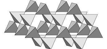
Figure 1: The pyrochlore lattice.

The absence of long range order does not mean the physics is trivial at low temperatures as the accessible states have non-trivial local constraints on them—hence cooperative paramagnet. For the thermodynamics it is possible to make do with small clusters, e.g. Pauling’s estimate of the entropy of ice works rather well and the thermodynamics of the Heisenberg pyrochlore magnet is well-described even by an approximation based on an isolated tetrahedronmoeberl . For the spin correlations however, the situation is presumably different. Indeed, Monte Carlo simulations of the Heisenberg magnet by Zinkin et al.zinkinmc have demonstrated the presence of sharp features in the structure factor in certain high symmetry directions (the “bow-ties” in Fig. 2), indicative of extended spin correlations. It is understood, qualitatively, that these are a direct consequence of the ground state constraint that each tetrahedron separately has vanishing total spinmoecha .

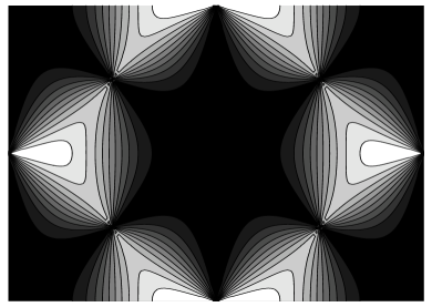
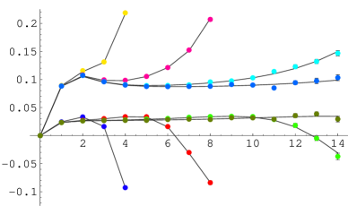
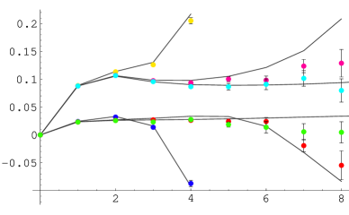
Figure 2: Top: The $[hhk]$ structure factor for $N=\infty$ [dark=low intensity; the x (y) axis corresponds to h (k)]. Middle: Ising correlations at $T=0$ (bottom: Heisenberg, at $T/J=0.005$) from Monte Carlo simulations, compared to $T=0$ large-$N$ correlations: $\langle S_{1}(x)S_{1}(0)\rangle$, for two inequivalent directions, $[101]$ and $[211]$, multiplied by the cube of the distance, $x^{3}$. The error bars are around $5\times 10^{-6}x^{3}$ ($5\times 10^{-5}x^{3}$). Different curves are for system sizes $L=8,16,32,48$ ($L=8,16,32$). There is no fitting parameter.

In this paper we provide a theory of the $T\rightarrow 0$ spin correlations of nearest neighbor $O(N)$ magnets on the pyrochlore lattice when they are paramagnetic down to $T=0$. This restriction excludes only the case $N=2$, but even there our results are probably applicable as we discuss below. Our work builds on two previous advances. The first is the recognitionyoungaxe3d ; clhu ; HKMS3ddimer ; hermele03 , generalizing work on two-dimensional iceyoungaxe , that $d=3$ models with binary degrees of freedom and a local “Gauss’s law” constraint should generally exhibit asymptotic dipolar correlations governed by a pure Maxwell action. This applies directly to our $N=1$ (Ising) case, while the underlying argument has been conjectured to apply also to Heisenberg spins by Henleyclhu . The second is the solution by Garanin and Canals of the $N=\infty$ limit canalsgaranin , in particular their numerical determination of the structure factor in the $N=\infty$ limit, which exhibits the same bow-ties observed by Zinkin et al.

In the following we (a) motivate how dipolar correlations arise in pyrochlore magnets from local constraints, (b) demonstrate their existence analytically in the $N=\infty$ limit and their persistence to all orders in the $1/N$ expansion, and (c) verify by simulation that the correlations at $N=3$ and $N=1$ are dipolar. We find that the correlations at $N=3$ are very well fitted by the $N=\infty$ formulae even without modifications at short distances. Remarkably we find that the $N=\infty$ formulae are probably even more accurate for $N=1$ where the relative and absolute error never exceed $2\%$ and $4.5\times 10^{-4}$, respectively even though this is not a conclusion that one would guess on the basis of the $1/N$ expansion! We close by noting the applicability of the ideas in the paper to related systems, which will be detailed in a separate publicationimswip , as well as their known limitations.

Local constraints and dipolar correlations: We consider the classical nearest neighbor antiferromagnet on the pyrochlore lattice, $H=J\sum_{\langle i,j\rangle}{\bf S}_{i}{\bf S}_{j}$, where the ${\bf S}_{i}$ are $N$-component spins of fixed length $N$. We set $J=1$ in the following. The pyrochlore lattice consists of corner sharing tetrahedra, and the Hamiltonian can be rewritten, up to a constant, as $H=(1/2)\sum_{\XBox}(\sum_{i\epsilon\XBox}{\bf S}_{i})^{2}$, where the sum in parentheses runs over all four spins at the corners of a given tetrahedron, $\XBox$, and the outer sum is over all tetrahedra. Hence, the ground states (minimum energy configurations) are such that for each tetrahedron and each spin component $\alpha$,

$$\sum_{i\in\XBox}S_{i}^{\alpha}=0.$$ (1)

This can be turned into a manifest conservation law on the dual – bipartite diamond – lattice, the sites of which are given by the centres of the tetrahedra while the spins sit at the midpoints of its bonds.

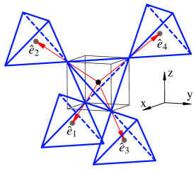
Figure 3: The centres of the tetrahedra define (the two sublattices of) the diamond lattice, denoted by black and grey dots. The orientation of the diamond bonds, and the four sublattices of the pyrochlore lattice, are defined by the vectors $\hat{e}_{\kappa}$

.

First, we orient each bond, $\kappa$, by defining a unit vector $\hat{e}_{\kappa}$, which points along the bond from one sublattice to the other, see Fig. 3. Next we define $N$ vector fields on each bond, ${\bf B}^{\alpha}_{\kappa}=S^{\alpha}_{\kappa}\hat{e}_{\kappa}$, where $S^{\alpha}_{\kappa}$ denotes the spin on bond $\kappa$. The ground state constraint (1) implies that each ${\bf B}^{\alpha}$ separately forms a set of solenoidal fields at $T=0$, $\nabla\cdot{\bf B}^{\alpha}=0$.

For $N=1$, spin flips connecting two ground states correspond to reversing the direction of a closed loop of “magnetic flux”, ${\bf B}$; evidently, ${\bf B}$ averages to zero over such a flippable cluster of spins. Upon coarse-graining, a high density of flippable clusters (and therefore a large number of ground states) translates into a small (well-averaged) coarse-grained ${\bf\tilde{B}}$. We now posit that this feature carries through to $N>1$, so that states with small values of ${\bf\tilde{B}^{\alpha}}$ will in general be (entropically) favoured. This is captured most simply by introducing a weight functional, $\rho$:

$$\rho[\{{\bf\tilde{B}}^{\alpha}({\bf x})\}]\propto\exp\left[-\frac{K}{2}\int d^{3}x\sum_{\alpha}({\bf\tilde{B}}^{\alpha})^{2}\right]$$ (2)

provided the solenoidal constraint is implemented, where $K$ is the stiffness constant. (If we solve the constaint by introducing a vector potential for each component, we are led to the Maxwell action.)

From this we can deduce the long distance correlators,

$$\langle\tilde{B}^{\alpha}_{i}({\bf x})\tilde{B}^{\beta}_{j}(0)\rangle\propto\delta_{\alpha\beta}{3x_{i}x_{j}-r^{2}\delta_{ij}\over r^{5}}$$ (3)

which are dipolar as advertised. The appropriate long-wavelenth formulae for the case $N=1$ have already been given in Ref. hermele03, .

This argument does not take into account thermal fluctuations out of the ground state manifold. These are gapped, and thus unimportant for $T\rightarrow 0$, for $N=1$. However, for continuous spins they endow each microscopic ground state with a non-trivial entropic weight, and are essential for even defining what is meant by a measure on the set of ground states. An analysis based on Maxwellian constraint counting implies that this weighting is sufficiently uniform to be innocuous for $N\geq 3$ so that the dipolar forms should hold. For $N=2$ this is not the case and the weighting leads to an order-by-disorder phase transition moecha ; fn-plane . However at this transition, the spins order collinearly but do not pick fixed orientations along their common axis. Hence, for the resulting collinear ensemble, the $N=1$ results can be applied, with the caveat that it has not been established whether a further phase transition will select a subset of collinear states at even lower temperatures.

While the arguments given above are based on the plausible ansatz (2), we now turn to establishing their actual correctness. The continuity of the physics for $N>3$ will allow us to tackle this in the $1/N$ expansion and we will supplement this with explicit simulation at small $N$.

$\bm{N}=\infty$: We start with the simple classical $O(N)$ model; its $N=\infty$ saddle pointmoshemoshe is, of course, the one discussed in Refs. canalsgaranin, . The partition function is given by $Z=\int{\cal D}\phi{\cal D}\lambda\exp[-{\cal S(\phi,\lambda)}]$, with the action defined as

$${\cal S(\phi,\lambda)} = \sum_{i,j}\sum_{\alpha=1}^{N}\frac{1}{2}\phi_{i}^{\alpha}A_{ij}\phi_{j}^{\alpha}+i\frac{\lambda_{i}}{2}\delta_{i,j}(\phi_{i}^{\alpha}\phi_{i}^{\alpha}-N)\ ,$$

where $A_{ij}$ is the interaction matrix divided by $T$.

The saddle point evaluation for $N=\infty$ is analogous to that of Refs. canalsgaranin, ; as we are not aware of an analytical treatment of the full pyrochlore correlations in the literature, we provide it here.

The Fourier transform of the interaction matrix is

$$2\left(\matrix{1&c_{xz}&c_{xy}&c_{yz}\cr c_{xz}&1&c_{\overline{yz}}&c_{\overline{xy}}\cr c_{xy}&c_{\overline{yz}}&1&c_{\overline{xz}}\cr c_{yz}&c_{\overline{xy}}&c_{\overline{xz}}&1}\right),$$ (4)

where $c_{ab}=\cos(\frac{{q_{a}}+{q_{b}}}{4})$ and $c_{\overline{ab}}=\cos(\frac{{q_{a}}-{q_{b}}}{4})$. The eigenvalues of the interaction matrix are reimersberlchi

$$\nu_{1,2}=0,\ \nu_{3,4}=2\pm\sqrt{1+Q},$$

where $Q=c_{xy}^{2}+c_{\overline{xy}}^{2}+c_{xz}^{2}+c_{\overline{xz}}^{2}+c_{yz}^{2}+c_{\overline{yz}}^{2}-3$.

These can be combined to give the spin correlatorscanalsgaranin . For the zero temperature case discussed here, only the modes with $\nu=0$ contribute. There are two independent correlators, namely those between spins on the same and between spins on different sublattices. We thus find the following spin correlators (we label four sublattices as shown in Fig. 3)

$$\langle S_{1}^{\alpha}({\bf q})S_{1}^{\beta}(-{\bf q})\rangle = \delta_{\alpha\beta}\frac{6-2c_{\overline{xy}}^{2}-2c_{\overline{xz}}^{2}-2c_{\overline{yz}}^{2}}{3-Q},$$

$$\langle S_{1}^{\alpha}({\bf q})S_{2}^{\beta}(-{\bf q})\rangle = \delta_{\alpha\beta}\frac{2\left(\cos(\frac{{q_{y}}}{2})c_{\overline{xz}}-c_{xz}\right)}{3-Q}\ .$$ (5)

From these one can calculate the correlators of ${\bf B}^{\alpha}=\sum_{\kappa}S^{\alpha}_{\kappa}\hat{e}_{\kappa}$ and verify that they have the small ${\bf q}$ forms,

$$\langle\tilde{B}^{\alpha}_{i}({\bf q})\tilde{B}^{\beta}_{j}({\bf q})\rangle\propto\delta_{\alpha\beta}(\delta_{ij}-\frac{q_{i}q_{j}}{q^{2}})$$ (6)

equivalent to the real space forms (3) noted earlier.

The structure factor in this limit is

$$S({\bf q})=4-\frac{8}{3-Q}\biggl{[}\left(c_{yz}+c_{\overline{yz}}\right){\sin^{2}\left(\frac{{q_{x}}}{4}\right)}$$ (7)

$$+ \left(c_{xz}+c_{\overline{xz}}\right){\sin^{2}\left(\frac{{q_{y}}}{4}\right)}+\left(c_{xy}+c_{\overline{xy}}\right){\sin^{2}\left(\frac{{q_{z}}}{4}\right)}\biggr{]}.$$

It has been customary to consider the structure factor of the pyrochlore antiferromagnets in the $[hhk]$ plane in reciprocal space, as it contains the high-symmetry directions $[100]$, $[110]$ and $[111]$. Here, the wavevector ${\bf q}=(q_{x},q_{x},q_{z})$, and Eq. 7 simplifies to

$$S_{[hhk]} = \frac{32{\left(\cos(\frac{{q_{x}}}{4})-\cos(\frac{{q_{z}}}{4})\right)}^{2}{\sin(\frac{{q_{x}}}{4})}^{2}}{5-\cos({q_{x}})-4\cos(\frac{{q_{x}}}{2})\cos(\frac{{q_{z}}}{2})}.$$ (8)

This is plotted in Fig. 2; the same plot has previously appeared in Ref. canalsgaranin, . We emphasize that it is the transverse, dipolar form of the correlators which gives rise to the bow tie structures.

$1/N$ expansion: To set up the $1/N$ expansion moshemoshe , we expand away from the saddle point by allowing the Lagrange multiplier field $\lambda$ to vary from its uniform saddle point value, $\tilde{\lambda}$: $\lambda_{i}=\tilde{\lambda}+\mu_{i}$. Integrating out the $\phi$’s removes the term linear in $\mu$; the quadratic term yields the propagator and higher order terms generate vertices. The quadratic term, $\sum_{ij}\mu_{i}\langle\phi_{i}\phi_{j}\rangle^{2}\mu_{j}\equiv\sum_{ij}\mu_{i}{\cal M}^{-1}_{ij}\mu_{j}$, implies a propagator $\langle\mu_{i}\mu_{j}\rangle={\cal M}_{ij}$. One can argue, and we have checked by explicit numerical computation, that $\langle\mu_{i}\mu_{j}\rangle$ decays inversely as the sixth power of the separation between $i$ and $j$. Hence its Fourier transforms, ${\cal M}_{\kappa\kappa^{\prime}}({\bf q})$, are continuous functions over the Brillouin zone. We note that the $N=\infty$ correlators of the spins $G^{0}_{\kappa\kappa^{\prime}}({\bf q})$ are discontinuous at ${\bf q}=0$ on account of their dipolar character.

We now briefly sketch the proof that the dipolar form on the spin correlations survives to all orders in the $1/N$ expansion; details will be presented in imswip . Consider the Dyson series for the spin correlator, $G$, at finite N:

$$G_{\kappa\kappa^{\prime}}({\bf q})=G^{0}_{\kappa\kappa^{\prime}}({\bf q})+G^{0}_{\kappa\kappa_{1}}({\bf q})\Sigma_{\kappa_{1}\kappa_{2}}({\bf q})G^{0}_{\kappa_{2}\kappa^{\prime}}({\bf q})+\cdots$$

where the self energy $\Sigma$ is the sum of the relevant graphs at all orders in $1/N$. For each graph that enters this sum one can show (I) that $\Sigma_{kl}({\bf q})$ is a continuous function of $q$ in the Brillouin zone, (II) that $\lim_{\bf q\rightarrow 0}\Sigma_{\kappa\kappa^{\prime}}({\bf q})=\sigma^{diag}$ for $\kappa=\kappa^{\prime}$ and $\sigma^{od}$ otherwise. (I) follows from the fact that in all such diagrams one integrates over an integrand that is bounded and at most discontinuous at isolated points, while (II) uses the action of lattice symmetries on $G^{0}$ and ${\cal M}$. Using these observations the leading small $q$ terms in the Dyson series lead to a simple geometric sum and one finds that

$$G_{\kappa\kappa^{\prime}}({\bf q})\propto G^{0}_{\kappa\kappa^{\prime}}({\bf q})$$ (9)

near ${\bf q}=0$. Consequently, the correlations are still dipolar at long distances. However, even in the most optimistic case we would not expect the series to converge beyond $N=3$, where long range order sets in due to order by disorder.

Comparison to Monte Carlo simulations: To the naked eye, the $N=\infty$ structure factor of Fig. 2 looks almost identical to the one obtained by Zinkin for Heisenberg spinszinkinmc and by us for Ising spinsimswip . For a more sensitive test we have compared the real-space expressions to Monte Carlo simulations for Ising and Heisenberg spins for different system sizes, shown in the same figure. We find that the error for Ising spins is very small indeed – the relative and absolute systematic error never seems to exceed $2\%$ and $4.5\times 10^{-4}$ respectively. The agreement for Heisenberg spins is somewhat worse. However, since the disagreement is of the size of the finite-temperature error bars, we cannot extrapolate down to $T\rightarrow 0$ reliably. In either case, one sees that the $N=\infty$ formulae we have derived work remarkably well quantitatively even without any further corrections—indeed, far better than one might have guessed at the outset—even at small distances, and they correctly capture finite-size effects.

Applicability to other models: As the Ising antiferromagnet on the pyrochlore lattice is isomorphic to (nearest-neighbour)enjgin spin ice, the results can straightforwardly be transcribed, and further carried over to cubic (water) ice $I_{h}$, which is again equivalentpyrowa . In the latter context the asymptotic form of the correlations is known youngaxe3d and the interest of our results is in the accuracy of our analytic forms at all distances. The analysis presented here straightforwardly generalises to other three dimensional cooperative paramagnets with conservation laws.

The present approach can also be applied to two-dimensional models with a conservation law. However, it breaks down for models with a discrete set of ground states. Technically, the effective height (two-dimensional gauge) field acquires a non-zero compactification radius in this case, which leads to the appearance of additional operators under coarse-graining. These are absent for $N=\infty$, and their appearance is non-perturbative in $N$. For the kagome magnet, for example, they arise for $N=2,3$, which is why the $\sqrt{3}\times\sqrt{3}$ correlations known to be present there were not found in Ref. canalsgaranin, . However, information gleaned from the present approach, such as a stiffness, can nonetheless usefully be fed into these models. Finally, we have shown that the present approach can also be applied to a class of paramagnetic models without a conservation law, for which so far very little has been known in terms of correlation functions. This, along with the more technical material, will be discussed elsewhereimswip .

Acknowledgements: We would like to thank Hans Hansson, Mike Hermele, Chris Henley, Anders Karlhede, Oleg Tchernyshyov and Kay Wiese for useful discussions. We are also grateful to David Huse and Werner Krauth for collaboration on closely related work. This work was in part supported by the Ministère de la Recherche et des Nouvelles Technologies with an ACI grant, by the NSF with grants DMR-9978074 and 0213706, and by the David and Lucile Packard Foundation.

References

- (1) P. W. Anderson, Phys. Rev. 102, 1008 (1956).
- (2) M. J. Harris et al., Phys. Rev. Lett. 79, 2554 (1997); A. P. Ramirez et al., Nature 399, 333 (1999).
- (3) J. Villain, Z. Phys. B 33, 31 (1979).
- (4) J. N. Reimers, Phys. Rev. B 45, 7287 (1992)
- (5) R. Moessner and J. T. Chalker, Phys. Rev. Lett. 80, 2929 (1998); Phys. Rev. B 58, 12049 (1998).
- (6) This is assuming the easy planes for all four sublattices coincide. For the case where they do not, see J. D. M. Champion and P. C. W. Holdsworth, J. Phys. Cond. Mat. 16, S665 (2004) and references therein.
- (7) R. Moessner and A. J. Berlinsky, Phys. Rev. Lett. 83, 3293 (1999)
- (8) M. P. Zinkin, M. J. Harris, and T. Zeiske, Phys. Rev. B 56, 11786 (1997)
- (9) R. W. Youngblood and J. D. Axe, Phys. Rev. B 23, 232 (1981).
- (10) C. L. Henley, unpublished.
- (11) D. A. Huse, W. Krauth, R. Moessner, and S. L. Sondhi, Phys. Rev. Lett. 91, 167004 (2003).
- (12) M. Hermele, M. P. A. Fisher, and L. Balents, Phys. Rev. B 69, 064404 (2004).
- (13) R. Youngblood, J. D. Axe, and B. M. McCoy, Phys. Rev. B 21, 5212 (1980).
- (14) D. A. Garanin and B. Canals, Phys. Rev. B 59, 443 (1999); B. Canals and D.A. Garanin, Can. J. Phys. 79, 1323 (2001).
- (15) S.V. Isakov et al., in preparation.
- (16) Our treatment follows the introduction to large- by M. Moshe and J. Zinn-Justin, Phys. Rep. 385, 69 (2003).
- (17) J. N. Reimers, A. J. Berlinsky, and A.C. Shi, Phys. Rev. B 43, 865 (1991).
- (18) For correlations in dipolar spin ice, see M. Enjalran and M. J. P. Gingras, cond-mat/0307151.