also at: ] Centro Interdipartimentale per lo Studio delle Dinamiche Complesse (CSDC), Università di Firenze, Istituto Nazionale per la Fisica della Materia (INFM), Unità di Ricerca di Firenze, and Istituto Nazionale di Fisica Nucleare (INFN), Sezione di Firenze, via G. Sansone 1, I-50019 Sesto Fiorentino (FI), Italy
also at: ] Centro Interdipartimentale per lo Studio delle Dinamiche Complesse (CSDC), Università di Firenze, Istituto Nazionale per la Fisica della Materia (INFM), Unità di Ricerca di Firenze, and Istituto Nazionale di Fisica Nucleare (INFN), Sezione di Firenze, via G. Sansone 1, I-50019 Sesto Fiorentino (FI), Italy
Topology and phase transitions: from an exactly solvable model to a relation between topology and thermodynamics
Abstract
The elsewhere surmised topological origin of phase transitions is given here new important evidence through the analytic study of an exactly solvable model for which both topology and thermodynamics are worked out. The model is a mean-field one with a -body interaction. It undergoes a second order phase transition for and a first order one for . This opens a completely new perspective for the understanding of the deep origin of first and second order phase transitions, respectively. In particular, a remarkable theoretical result consists of a new mathematical characterization of first order transitions. Moreover, we show that a “reduced” configuration space can be defined in terms of collective variables, such that the correspondence between phase transitions and topology changes becomes one-to-one, for this model. Finally, an unusual relationship is worked out between the microscopic description of a classical -body system and its macroscopic thermodynamic behaviour. This consists of a functional dependence of thermodynamic entropy upon the Morse indexes of the critical points (saddles) of the constant energy hypersurfaces of the microscopic -dimensional phase space. Thus phase space (and configuration space) topology is directly related to thermodynamics.
pacs:
05.70.Fh; 02.40.-k; 75.10.HkI Introduction
Thermodynamical phase transitions are certainly one of the main topics of statistical physics. A huge amount of work, both theoretical and experimental, has been done during the past decades leading to remarkable successes as is witnessed, for example, by the Renormalization Group theory of critical phenomena. However, there are still longstanding open problems about phase transitions; among them we can mention amorphous and disordered systems (like glasses and spin-glasses) undergoing “dynamical” transitions, or first-order phase transitions, which are still lacking a satisfactory theoretical understanding of their origin. Moreover, on the forefront of modern research in statistical physics, standard theoretical definitions and methods are challenged by the experimentally observed phase transitions occurring in small classical and quantum systems (nano and mesoscopic) like atomic and molecular clusters, polymers and proteins, Bose-Einstein condensates, droplets of quantum liquids, etc. Finally, in the mathematically rigorous background of phase transitions theory, neither in the Yang-Lee theory for the grandcanonical ensemble YL nor in the Ruelle, Sinai, Pirogov theory for the canonical ensemble RS , an a-priori mathematical distinction can be made among the potentials leading to first or second order phase transitions, respectively.
The present paper aims to contribute to the advancement of a recently proposed theoretical framework where the singular behaviours of thermodynamic observables at a phase transition are attributed to major topology changes in phase space and – equivalently – in configuration space cccp ; franzosi ; phi4 ; physrep ; xy . More precisely, in Ref. cccp ; franzosi ; phi4 ; physrep ; xy , it has been proposed that thermodynamic phase transitions could be a consequence of suitable topology changes of certain submanifolds of the configuration space defined by the potential energy function. The presence of such topological changes has been recently shown to be a necessary condition, under fairly general assumptions, for the presence of a phase transition theorem ; however, the converse is not true, and no rigorous results are available yet on the sufficient conditions. The analytical or numerical study of particular models thus remains crucial to get hints towards more general results (see also Refs. grinza ; kastner for recent results on one-dimensional systems, and Ref. ribeiro as to the fully connected spherical model).
In this perspective, we stress that the topological approach has been hitherto applied only to systems undergoing second-order phase transitions. Therefore tackling first order phase transitions in the topological framework is of great interest, because some new insight into the challenging problem of their origin can be obtained, and because this reinforces the working hypothesis that the topological approach could unify the treatment of the different kinds of phase transitions in view of encompassing also more “exotic” ones, like glassy transitions and the others mentioned above.
In this paper we first study a model which, according to the value of a parameter, has no transition or undergoes a first or a second order transition. Remarkably, for this model an exact analytical computation is possible of the Euler characteristic – that is a topological invariant – of those submanifolds of the configuration space whose topological changes are expected to be related to the phase transition. We find epl2003 that the phase transition is actually signaled by a discontinuity in the Euler characteristic and that the sign of the second derivative of indicates the order of the transition. Then, we study the topology of submanifolds of a “reduced” configuration space, i.e., the space of some collective variables: in this case we find a one-to-one correspondence between phase transitions and topology changes.
Finally, we derive a general result showing that an analytic estimate of another topological invariant of the same submanifolds can be worked out which allows to directly link topology and thermodynamic entropy.
II A key study
In this Section we present a study of the thermodynamical properties of the mean-field -Trigonometric Model (TM), as well as of the topological properties of its configuration space. A preliminary study of this model along these lines has already been reported in epl2003 ; there only the microcanonical thermodynamics was considered, while here we are going to discuss also the canonical thermodynamical properties. Being a model with long-range interactions which may undergo also first-order phase transitions, we expect canonical and microcanonical thermodynamic functions to be different, at least close to first-order transitions ruffobook .
The TM is defined by the Hamiltonian:
| (1) |
where are angular variables: , are the conjugated momenta, and the potential energy is given by
| (2) |
where is the coupling constant. In what follows only the potential energy part will be considered. This interaction energy is apparently of a mean-field nature, in that each degree of freedom interacts with all the others; moreover, the interactions are -body ones.
The TM is a generalization of the Trigonometric Model (TM) introduced by Madan and Keyes MK as a simple model for the Potential Energy Surface (PES) – the hypersurface defined by the potential energy as a function of the degrees of freedom – of simple liquids. The TM is a model for independent degrees of freedom with potential energy (2) with : .
It shares with Lennard-Jones like systems lj_sad the existence of a regular organization of the critical points of the potential energy above a given minimum (the elevation in energy of the critical points is proportional to their index) and a regular distribution of the minima in the configuration space (nearest-neighbor minima lie at a well defined Euclidean distance). The PES of the TM maintains the main features of the TM ktm , introducing however a more realistic feature, namely the interaction among the degrees of freedom (in the form of a -body interaction).
Using the relation
| (3) |
the configurational part of the Hamiltonian can be written as
| (4) | |||||
where and are collective variables, functions of :
| (5) | |||||
We observe also that the model has a symmetry group obtained by the transformations
| (6) |
If we think of as the angle between a unitary vector in a plane and the horizontal axis of this plane, we find that the first transformations are rotations in this plane of an angle and the second is the reflection with respect to the horizontal axis. This group is also called .
Let us now derive the thermodynamical properties of the TM.
II.1 Canonical thermodynamics
The partition function is
| (7) |
introducing -functions for the variables and ,
| (8) |
and using the integral representation of the -function, we obtain for
| (9) |
The last integral is easily computable using Eq. (5),
| (10) |
and can be written in term of the Bessel function
| (11) |
where , , and . The partition function can then be written as
| (12) |
and since the function is always positive, there are no problems in defining its logarithm.
We want now to perform a saddle-point evaluation of the integral, so we have to look for the minima of the exponent in the complex plane. We note that if that points do not lie on the imaginary axis of the planes, the free energy of the model would be imaginary. So we can safely rotate the integration path on the imaginary axis in the planes, which corresponds to the substitutions: and , then and , where is the modified Bessel-function:
| (13) |
In conclusion we obtain
| (14) |
where is the real function
| (15) |
In order to find the stationary points, we first determine the subspace defined by the equations
| (16) | |||
| (17) |
obtaining the relations
| (18) | |||||
| (19) |
thus we get
| (20) |
Now, using Eqs. (18,19), we can substitute and with and in Eq. (15), obtaining, in term of the complex number ,
| (21) |
and using the polar representation
| (22) |
The derivative with respect to leads to
| (23) |
so that there are solutions
| (24) |
Observing that we obtain
| (25) |
and we can restrict ourselves to . Finally, the derivative with respect to leads to the stationary points equation:
| (26) |
where the modified Bessel-function is defined by
| (27) |
For we have only the trivial solution , because the functions are always positive. By using an expansion for small one can show that this solution is a maximum for . So we can study only the case . We note that if there is a non trivial solution (i.e., ) of Eq. (26), calling the value of , we have
| (28) |
and the free energy and internal energy are, respectively,
| (29) | |||||
| (30) |
Let us now analyze the case . In this case the solutions are not present, so that we have only the solution
| (31) |
There is no phase transition, and using Eq. (30) we have
| (32) |
This is the free energy of trigonometric model that has been mentioned before.
For the solution is stable for high temperatures, but a non trivial solution of Eq. (26) appears at . The transition temperature is given by the condition
| (33) |
so that we obtain ; the transition is continuous, and the order parameter is . It is easy to show that and (e.g., by adding an external field of the form to the Hamiltonian and performing the limit ); then the vector is the mean magnetization of the spins represented by the . As is the modulus of the magnetization, for , when , the symmetry is broken.
When , the non trivial solution of Eq. (26) appears at a given but becomes stable only at , so that and are discontinuous at ; instead of the instability region , in the microcanonical ensemble a region where the specific heat is negative appears, as we shall see below. The symmetry is broken in the low temperature phase, so that can be used as an order parameter in revealing the symmetry breaking, even if it is not continuous at . The transition is then of first order, but keeps the symmetry structure of a second order one, i.e., in the low temperature phase there are pure states related by the symmetry group also in the case of the first order transition.
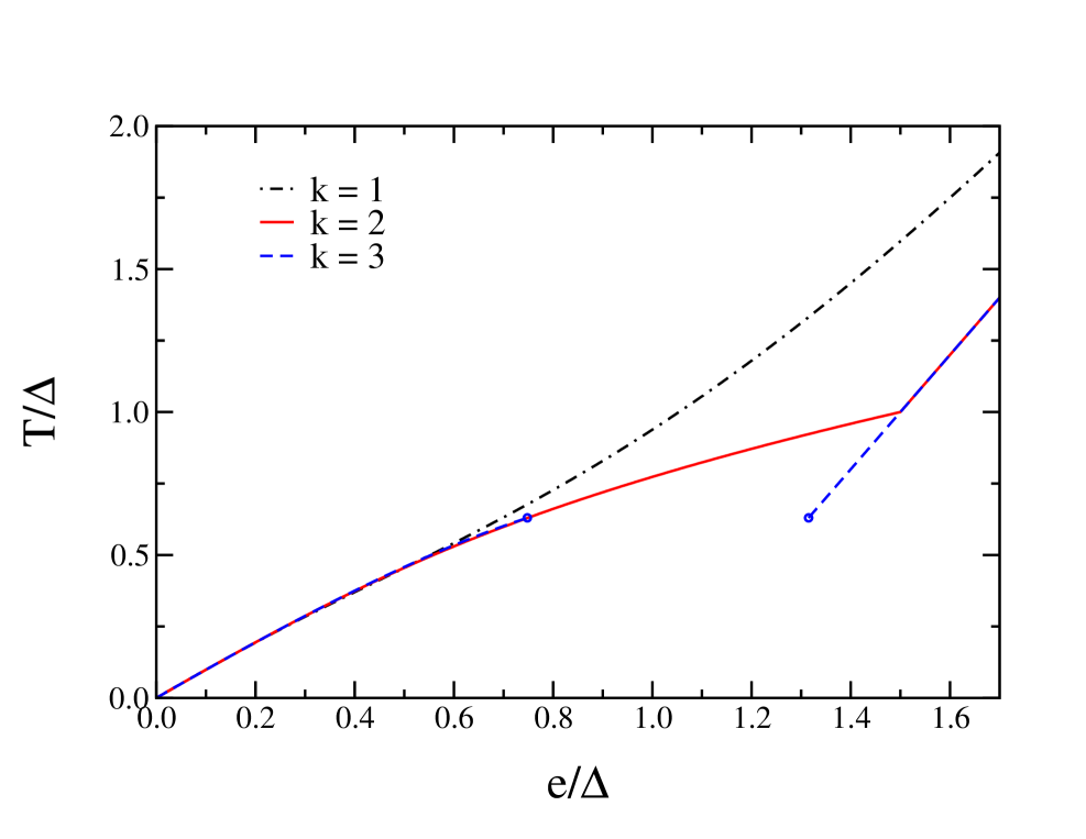
In Fig. 1 we report the caloric curve, i.e., the temperature as a function of the average energy (per degree of freedom) , for three values of , , 2 and 3. As previously discussed, the temperature is an analytic function of for ; for the system undergoes a second order phase transition at a critical temperature , that changes to first order for .
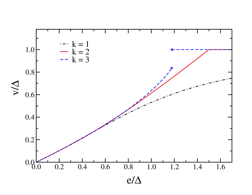
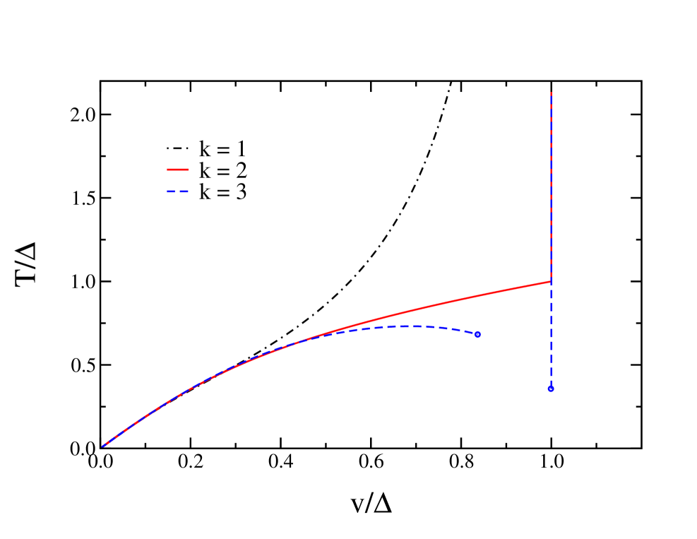
In Figs. 2 and 3 we report the average potential energy as a function of the average energy and the temperature as a function of , respectively. It is apparent that, for , the phase transition point always corresponds to .
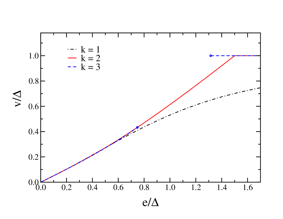
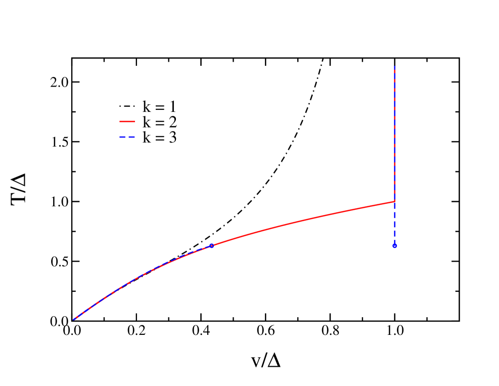
Another feature which shows up in Figs. 2 and 3 is that the average potential energy never exceeds the value , i.e., although the maximum of is equal to , the region is not thermodynamically accessible to the system. The reason for this is in the mean-field nature of the system and in the fact that we are working in the thermodynamic limit . According to Eqs. (4), the potential energy can be written as a function of the collective variables and defined in Eqs. (5), which are the components of the function whose statistical average is the order parameter, i.e., the “magnetization”. In the thermodynamic limit these functions become constants, whose value coincides with their statistical average, and since for , and from Eqs. (4) this implies for all .
As we shall see below, this fact remains true also in the microcanonical ensemble, which, however, is not equivalent to the canonical ensemble for the present model, due to the long-range nature of the interactions.
II.2 Microcanonical thermodynamics
As in other simple mean field models, also in the case of the TM it is possibile to perform a calculation of the microcanonical partition function, or microcanonical density of states in phase space, given by
| (34) |
The computation of is similar to that of in the canonical case, so that we will go through it with less detail.
Using the integral representation of the delta function, we get
| (35) |
Now, as we are looking for a saddle-point evaluation of the integral over , we can rotate the integration path on the imaginary axis in the complex- plane. This is justified because, as in the canonical case, the saddle-point is located on this axis. We can now perform the integration over the momenta and use the fact that , see Eq. (4), to obtain
| (36) | |||||
where and the constant gives only a constant contribution to the entropy per particle, i. e., it is at most of order . The last integral can be evaluated using again the integral representation of the delta function, and rotating then the integration path as previously discussed; it turns out to be:
having defined ; is a Bessel function as before. We can then write the density of states as
| (37) |
where , and
Then, using the saddle-point theorem, the entropy per particle, , is given by (=1):
| (38) |
To find the maximum of one can calculate analytically some derivatives of to obtain a one-dimensional problem that can be easily solved numerically with standard methods.
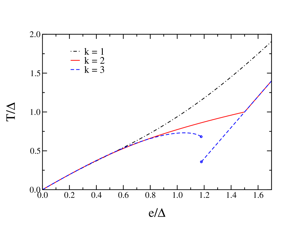
As already done in the case of the canonical ensemble, in Fig. 4 we report the microcanonical caloric curve, i.e., the temperature as a function of the energy (per degree of freedom) , for three values of , , 2 and 3. As in the canonical case, the temperature is an analytic function of for , while for =2 the system undergoes a second order phase transition at a certain energy value , that changes to first order for .
We note that, for , in a region of energies smaller than the critical energy of the first-order phase transition the curve has a negative slope, i.e., the system has a negative specific heat. The TM is then another physical model where this feature is found (see, e.g., Ref. ruffobook for other examples). This is not surprising at all since we are considering the microcanical thermodynamics of a system with long-range interactions; such a region is not present when we consider the canonical ensemble, as shown above; there, the region of negative specific heat corresponds to the region of instability of the non-trivial solution of the saddle-point equations.
In Figs. 5 and 6 we report the average microcanonical potential energy as a function of and the microcanonical temperature as a function of , respectively. It is apparent that, for , the phase transition point always corresponds to .
As in the canonical case, the average potential energy never exceeds the value , i.e., the region is not thermodynamically accessible to the system also in the microcanonical ensemble.
II.3 Topology of configuration space
In this Section we want to investigate the relation between the phase transitions occurring in the TM and the topology of its configuration space. Given the potential energy , the following submanifolds of configuration space are defined:
As varies from the minimum to the maximum allowed value of , the manifolds progressively cover the whole configuration space. These submanifolds, or their boundaries , are then a possible way to depict the potential energy landscape of the system. The topology of the ’s can be studied using Morse theory morse : whenever a critical value of – i.e., a value corresponding to one or more critical points, where the differential of vanishes – is crossed, the topology of the ’s change. It has been conjectured cccp ; physrep that some of these topology changes are the “deep” cause of the presence of a phase transition. The correspondence between major topology changes of the ’s and ’s and phase transitions has been checked in two particular models phi4 ; xy ; more recently, it has been proved theorem that a topology change is a necessary condition for a phase transition under rather general assumptions111Mean-field models with long-range interactions, like those to be analyzed in the present paper, do not rigorously fulfill the hypotheses of the theorem proved in theorem ; the fact that we do find a correspondence between the phase transition and a particular topology change also for these models, as already found in other models with long-range interactions, suggests that the theorem could be probably extended to a wider class of systems, which however would not necessarily include all the possible kinds of models with long-range, mean-field-like interactions (see also the discussion in Sec. IV)., but the sufficiency conditions are still lacking.
A natural way to characterize topology changes involves the computation of some topological invariants of the manifolds under investigation. One of such invariants is the Euler characteristic : in xy ; phi4 it was shown that the Euler characteristic of the submanifolds and/or of the shows a singularity in correspondence of the potential energy value at which the transition takes place: this seems then to signal a particularly “strong” topology change. Remarkably, the Euler characteristic of can be calculated analytically in our model. The general definition is nakahara :
| (39) |
where the Morse numbers are the number of critical points of index of the function that belong to the manifold . As already mentioned, the critical points (called saddles in other contexts, e.g., in the physics of glasses) are defined by the condition , and their index (otherwise called the order of the saddle) is defined as the number of negative eigenvalues of the Hessian matrix
| (40) |
To be valid, Eq. (39) requires that is a Morse function, i.e., that its critical points are nondegenerate: this means that all the eigenvalues of the Hessian are nonzero at a critical point and that the critical points themselves are isolated.
To determine the critical points we have then to solve the system
| (41) |
that is, inserting Eq. (4) in the equations above,
| (42) |
where we defined . From Eq. (4) we have
| (43) |
then all the critical points with have energy . We note that they correspond to vanishing magnetization. Let us now consider all the critical points with . Then Eq. (42) becomes
| (44) |
and its solutions are
| (45) |
where . Since in Eq. (42) appears to the -th power, in the case Eqs. (42) and (44) coincide. This means that the solutions given in Eq. (45) are all the critical points, regardless of their energy, in the case and all the critical points but those with energy in the case . The critical point is then characterized by the set . To determine the unknown constant we have to substitute Eq. (45) in the self-consistency equation
| (46) |
If we introduce the quantity defined by
| (47) |
which means
| (48) |
we have from Eq. (46)
| (49) | |||
| (50) |
where . Then the choice of the set is not sufficient to specify the set , because the constant can assume some different values. This fact is connected with the symmetry structure of the potential energy surface: the different values of correspond to the symmetry-related critical points under the group .
We can then state that all the critical points with – whose energy – have the form
| (51) |
The Hessian matrix is given by
| (52) | |||||
In the thermodynamic limit it becomes diagonal
| (53) |
One can not a priori neglect the contribution of the off-diagonal terms to the eigenvalues of , but we have numerically checked that their contribution change at most the sign of only one eigenvalue over : we note that in the case of the mean-field model this result has been proven explicitly xy . Neglecting the off-diagonal contributions, the eigenvalues of the Hessian calculated in the critical point are obtained substituting Eq. (51) in Eq. (53):
| (54) |
so the index of the critical point is simply the number of in the set ; we can identify the quantity given by Eq. (47) with the fractional index of the critical point . Then, from Eq. (4), (49) and (50) we get a relation between the fractional index and the potential energy at each critical point :
| (55) |
Moreover, the number of critical points of given index is simply the number of way in which one can choose times 1 among the , see Eq. (51), multiplied for a constant that takes into account the degeneracy introduced by Eq. (50).
We have then completely characterized the critical points with . Now we are going to argue that, in order to compute the Euler characteristic of the manifolds , we can neglect the critical points with , thus showing that the knowledge of the critical points considered so far is sufficient. The critical points with are degenerate: the Hessian vanishes at these points. This means that the potential energy is no longer a proper Morse function when , and we could use its critical points to compute the Euler characteristic of the manifolds only when . To overcome this difficulty we reason as follows. Morse functions are dense in the space of smooth functions: this means, in practice, that if a function is not a Morse function, any small perturbation will make it a proper Morse function MorseCairns , and we can consider, as our Morse function, the function , i.e., the potential energy plus a linear term which can made as small as we want:
| (56) |
where . The perturbation changes only slightly the critical points with , but completely removes the points with for any , no matter how small. All the critical points of this function are given by the solutions of the equations
| (57) |
which are only a slight deformation of Eqs. (44), so that provided all the ’s are very small the numerical values of critical points and critical levels will essentially coincide with those computed so far, in the case but assuming .
The fractional index of the critical points is a well defined monotonic function of their potential energy , given by Eq. (55), and the number of critical points of a given index is . Then the Morse indexes of the manifold are given by if and 0 otherwise, and the Euler characteristic is
| (58) |
using the relation .
In Fig. 7 we plot , that, from Eq. (58), is given by:
| (59) |
It has to be stressed that is a purely topological quantity, being related only to the properties of the potential energy surface defined by , and, in particular, to the energy distribution of its saddle points. From Fig. 7 we can see that there is an evident signature of the phase transition in the analytic properties of . First, we observe that the region is never reached by the system, as discussed before and showed in Figs. 5 and 6 as to the microcanonical case, and in Figs. 2 and 3 as to the canonical case; this region is characterized by . The main observations are that: for =1, where there is no phase transition, the function is analytic; for =2, when we observe a second order phase transition, the first derivative of is discontinuous at , and its second derivative is negative around the singular point. for the first derivative of is also discontinuous at the transition point , but its second derivative is positive around . In this case a first order transition takes place. Therefore the investigation of the potential energy topology, via , allows us to establish not only the location but also the order of the phase transitions, without introducing any statistical measure.
The previous results suggest us to conjecture that there is a relation between the thermodynamic entropy of the system and the topological properties of the potential energy landscape, as probed by . We recall that the presence of a first order transition with a discontinuity in the energy is generally related gallavotti to a region of negative specific heat, i.e., of positive second derivative of the entropy. Thus, it seems that at least around the transition point the thermodynamic entropy and are closely related: more precisely, it seems that the jump in the second derivative of is determined by the jump in the second derivative of . Then it should be possible to write
| (60) |
where is analytic (or, at least, ) around the transition point.
In Sec. III we explain how such a link between thermodynamics and topology could be obtained. But before doing so we show a different way of looking at the topology of the submanifolds of configuration space defined by the potential energy.
II.4 Topology of the order parameter space
A feature of many mean-field models (although not of all of them) is that the potential energy can be written as a function of a collective variable, whose statistical average is the order parameter. In the case of the -trigonometric model this variable is the two-dimensional “magnetization” vector defined as , where (see Eqs. 5)
| (61) |
Written in terms of , the potential energy is a function defined on the unitary disk in the real plane, which is given by (see Eq. (4))
| (62) |
In the particular cases the potential energy reads as
| (63) | |||||
| (64) | |||||
| (65) |
and it is then natural to investigate the topology of the ’s seen as submanifolds of the unitary disk in the plane, i.e., we now consider the submanifolds
| (66) |
where . The ’s are nothing but the ’s projected onto the “magnetization” plane.
The topology of these manifolds can be studied directly, by simply drawing them. In the case , where no phase transition is present, no topology changes occur in the ’s, i.e., all of them are topologically equivalent to a single disk (Fig. 8). When , and a phase transition is present, there is a topology change precisely at , where disks merge into a single disk (see Figs. 9 and 10). The detail of the transition, i.e., the number of disks which merge into one, clearly reflects the nature of the symmetry breaking for the particular value of considered (similar pictures are obtained for ). Thus, when projected onto the order parameter space, the correspondence between topology changes and phase transitions becomes one-to-one (this was already found in xymf for the mean-field model); however, at variance with the study of the topology of the “full” ’s, no direct way to discriminate between first- and second-order transitions seems available in this picture.


III Topology and thermodynamics: a direct link
We now show how it is possible to establish a general relationship between topology and thermodynamics. This can be achieved by improving some preliminary results on the subject reported in franzotesi ; CSCP .
Consider a generic classical system described by a Hamiltonian
where and the symbols have standard meaning. Then consider the microcanonical entropy defined as
| (67) |
where , where we shall put and where
| (68) |
with , i.e., is the microcanonical density of states. Here is the constant-energy hypersurface in the -dimensional phase space corresponding to the total energy , that is .
From the general derivation formula laurence
| (69) |
where is an integrable function and is the operator
the following result is worked out
| (70) |
where . is directly proportional to the mean curvature of seen as a submanifold of docarmo according to the simple relation . By integrating equation Eq. (70) we obtain the following equivalent expression for
| (71) |
and then, at large , considering that the volume measure concentrates on the boundary , we write
| (72) | |||||
where, in the last approximate replacement, we have used that is positive and only very weakly varying at large .
By means of Hölder’s inequality for integrals we get
the sign of equality being better approached when is everywhere positive. Hence, using Eqs. (68), (71) and (72)
| (73) |
and introducing a suitable deformation factor we can write
| (74) |
so that
| (75) |
where we have used , with the principal curvatures of , and is the Gauss-Kronecker curvature of , . is a remainder. Again we have used that is only very weakly varying at large and that it is always positive.
According to the Chern-Lashof theorem chernlashof
| (76) |
where is an -dimensional hypersphere of unit radius and are the Morse indexes of which are defined exactly as those of the ’s seen in the previous Sections, i.e., as the number of critical points of index on a given level set ; a critical point is a point where , the index of a critical point is the number of negative eigenvalues of the Hessian of computed at the critical point.
Finally the entropy per degree of freedom reads as
| (77) | |||||
The meaning of Eq. (77) is better understood if we consider that the Morse indexes of a differentiable manifold are related to the Betti numbers of the same manifold by the inequalities
| (78) |
The Betti numbers are fundamental topological invariants nakahara of differentiable manifolds; they are the diffeomorphism-invariant dimensions of suitable vector spaces (the de Rham’s cohomology spaces), thus they are integer numbers. The equality sign holds only for the so-called perfect Morse functions, which are rare, however, at large dimension we can safely replace Eq. (78) with (see e.g. Refs. xy ).
Equation (77), rewritten as
| (79) | |||||
links topological properties of the microscopic phase space with the macroscopic thermodynamic potential .
In particular, even though the function is unknown, sudden changes of the topology of the hypersurfaces (reflected by the energy variation of ) necessarily affect the energy variation of the entropy.
Finally, we resort to the fact that – at large – the volume measure of concentrates on , where is the kinetic energy hypersphere and , so that can be approximated by this product manifold, and we resort to the Kunneth formula nakahara for the Betti numbers of a product manifold , i.e.
| (80) |
which, applied to , gives for , and for , since all the Betti numbers of an hypersphere vanish but and which are equal to nakahara . Eventually we obtain
| (81) | |||||
where stands for the integral on the product manifold of the remainder which appears in Eq.(79). The equation above makes explicit the fact that the kinetic energy term of a standard Hamiltonian is topologically trivial.
From this equation we see that a fundamental topological quantity, the sum of the Betti numbers of the submanifolds of configuration space, is related, although with some approximation, to the thermodynamic entropy of the system.
While a relationship between topology and thermodynamics exists, as is shown by both Eqs. (81) and (77), an analytic formula linking the Euler characteristic to thermodynamics has not been found yet and is unlikely to exist. Therefore, in those cases allowing the analytic computation of the Morse indexes (as for the models tackled in this paper), besides the computation of the Euler characteristic through the formula (39), we can use the Morse indexes to replace the sum in Eq. (81) with , having resorted again to the estimate . Then we can plot this sum, that we shall denote by , against the potential energy density for the three different cases considered: . The result is shown in Fig. 11, where sharp differences are evident between the three situations: i) , absence of any phase transition, in which case the pattern of vs is smooth; ii) , second order phase transition, in which case the pattern of vs displays a sharp non-differentiable change at the phase transition point; iii) , first order phase transition, in which case the pattern of vs again displays a sharp non-differentiable change at the phase transition point which is approached from the left with an opposite concavity with respect to the second order transition case. Likewise the Euler characteristic, the quantity is in one-to-one correspondence with topology changes of the manifolds , but has the advantage of being directly related with thermodynamic entropy.
Both the general analytic result of Eq. (81) and the particular analytic result obtained for the TM and reported in Fig. 11 are of great relevance in view of a deeper understanding of the relationship between topology changes of configuration space and phase transitions: further work is ongoing along this direction.
As a final comment, let us remark that the clearcut differences among the three different cases in Fig. 11 are detected prior to and independently of the definition of any statistical measure in configuration space: the relevant information about the macroscopic physical behavior is already contained in the microscopic interaction potential itself and concealed in its way of shaping configuration space submanifolds.
IV Concluding remarks
We have presented a mean-field model whose thermodynamics is exactly solvable in both the canonical and the microcanonical ensemble: the model depend on a parameter and exhibits no transitions, a continuous phase transition and a discountinuous one, in the cases , , and , respectively. For this model, a clear and sharp relation between the presence of a phase transition and a particular topology change in the submanifolds of the -dimensional configuration space is analytically worked out: this correspondence becomes one-to-one if we look at the submanifolds of a reduced two-dimensional configuration space spanned by collective variables. Moreover, not only the presence and the location in energy of the transition can be inferred by looking at the behavior of topological quantities: also the order of the transition is related to the behavior of a topological invariant of the above mentioned submanifolds, their Euler characteristic. This suggests that topological quantities are linked in general to thermodynamic observables. Such a general link, although based on some approximations, has been derived in the final Section of the paper.
The results presented here confirm the validity and the potential of the topological approach to phase transitions, which has recently received a rigorous background via the proof of a theorem theorem stating that, for systems with short-ranged interactions, topology changes in the submanifolds of configuration space are a necessary condition for a phase transition to take place. The model we studied here is not short-ranged, thus the theorem might probably be extended to a more general class of systems. However, we would like to mention the case of a mean-field model, the fully coupled model, which has been recently studied phi4mf , and where the relation between the topology changes in the submanifolds of the configuration space and the phase transition is less straightforward. Further work is then needed to assess the full potential and the limits of the topological approach to phase transitions.
References
- (1) C. N. Yang and T. D. Lee, Phys. Rev. 87, 404 (1952); T. D. Lee and C. N. Yang, Phys. Rev. 87, 410 (1952).
- (2) H. O. Georgii, Gibbs measures and Phase Transitions, (de Gruyter, New York, 1988).
- (3) L. Caiani, L. Casetti, C. Clementi, and M. Pettini, Phys. Rev. Lett. 79, 4361 (1997).
- (4) R. Franzosi, L. Casetti, L. Spinelli, and M. Pettini, Phys. Rev. E 60, R5009 (1999).
- (5) R. Franzosi, M. Pettini, and L. Spinelli, Phys. Rev. Lett. 84, 2774 (2000).
- (6) L. Casetti, M. Pettini, and E. G. D. Cohen, Phys. Rep. 337, 237 (2000).
- (7) L. Casetti, E. G. D. Cohen, and M. Pettini, Phys. Rev. E 65, 036112 (2002); L. Casetti, M. Pettini, and E. G. D. Cohen, J. Stat. Phys. 111, 1091 (2003).
- (8) R. Franzosi and M. Pettini, Phys. Rev. Lett. 92, 060601 (2004); R. Franzosi, M. Pettini, and L. Spinelli, arXiv:math-ph/0305032, submitted to Commun. Math. Phys. (2003).
- (9) P. Grinza and A. Mossa, Phys. Rev. Lett. 92, 158102 (2004).
- (10) M. Kastner, arXiv:cond-mat/0404511.
- (11) A. C. Ribeiro-Teixeira and D. A. Stariolo, arXiv:cond-mat/0405421, Phys. Rev. E (2004, to appear).
- (12) L. Angelani et al., Europhys. Lett. 62, 775 (2003).
- (13) Dynamics and thermodynamics of systems with long-range interactions, T. Dauxois et al., eds. (Telos, 2003).
- (14) B. Madan and T. Keyes, J. Chem. Phys. 98, 3342 (1993).
- (15) L. Angelani et al., Phys. Rev. Lett. 85, 5356 (2000); J. Chem. Phys. 116, 10297 (2002); L. Angelani et al., J. Chem. Phys. 119, 2120 (2003).
- (16) L. Angelani, G. Ruocco, and F. Zamponi, J. Chem. Phys. 118, 8301 (2003); F. Zamponi et al., J. Phys. A: Math. Gen. 36 8565 (2003).
- (17) J. Milnor, Morse theory (Princeton University Press, Princeton, 1963); Y. Matsumoto, An introduction to Morse theory (AMS, Providence, 2002); an elementary summary of Morse theory is also given in Ref. physrep .
- (18) M. Nakahara, Geometry, Topology and Physics, (Adam Hilgher, Bristol, 1991).
- (19) M. Morse and S. S. Cairns, Critical Point Theory in Global Analysis and Differential Topology (Academic Press, New York, 1969); see in particular Theorem 6.4’ on page 48.
- (20) G. Gallavotti, Statistical mechanics (Springer, Berlin, 1999).
- (21) L. Casetti, E. G. D. Cohen, and M. Pettini, Phys. Rev. Lett. 82, 4160 (1999).
- (22) R. Franzosi, PhD thesis (Università di Firenze, 2000).
- (23) M. Cerruti-Sola, C. Clementi and M. Pettini, Phys. Rev. E 61, 5171 (2000).
- (24) P. Laurence, ZAMP 40, 258 (1989).
- (25) M. P. Do Carmo, Riemannian geometry (Birkhäuser, Boston - Basel, 1993).
- (26) S. S. Chern and R. K. Lashof, Michigan Math. J. 5, 5 (1958).
- (27) F. Baroni, Laurea thesis (Università di Firenze, 2002); A. Andronico et al., arXiv:cond-mat/0405188; D. A. Garanin, R. Schilling and A. Scala, arXiv:cond-mat/0405190.