Statistical characterization of the forces on spheres in an upflow of air

Abstract

The dynamics of a sphere fluidized in a nearly-levitating upflow of air were previously found to be identical to those of a Brownian particle in a two-dimensional harmonic trap, consistent with a Langevin equation [Ojha et al., Nature 427, 521 (2004)]. The random forcing, the drag, and the trapping potential represent different aspects of the interaction of the sphere with the air flow. In this paper we vary the experimental conditions for a single sphere, and report on how the force terms in the Langevin equation scale with air flow speed, sphere radius, sphere density, and system size. We also report on the effective interaction potential between two spheres in an upflow of air.

I Introduction

One of the great challenges in physics today is to understand the dynamics of driven nonequilibrium systems Ruelle (2004). This is particularly important in soft-matter physics, because the materials often have a delicate mesoscopic structure that is easily perturbed far from equilibrium. There, an understanding of the microscopic dynamics is crucial for a fundamental understanding of macroscopic behavior. Granular materials are an excellent example of this point Jaeger et al. (1996); Duran (2000). When subjected to strong driving forces, granular systems exhibit gas- or liquid-like behavior at the macroscopic scale and strong velocity fluctuations and collisions at the grain-scale. The microscopic fluctuations are created by the act of flowing, and, at the same time, are responsible for the dissipation that limits the rate of flow. The difficulty of treating the fluctuations is one reason why granular mechanics remains a forefront research topic, and why engineering systems are alarmingly prone to failure.

One way to characterize the microscopic dynamics in a granular gas or liquid is by the distribution of speed fluctuations. This has a long history, and is associated with attempts to develop a system of partial differential equations describing granular hydrodynamics Bagnold (1954); Ogawa (1979); Jenkins and Savage (1983); Haff (1983); Reydellet et al. (2000); Bocquet et al. (2002). The average kinetic energy associated with speed fluctuations has come to be known as the “granular temperature”, in loose analogy with kinetic theory of gases. An interesting line of research has been to explore the extent to which this analogy holds, i.e. the extent to which statistical mechanical concepts for true thermal systems can be used to describe granular fluctuations. For dilute or two-dimensional systems it is relatively straightforward to track grain motion by video techniques. Experimentalists have thus studied whether or not speed distributions are Gaussian, and whether or not equipartion is obeyed Pouligny et al. (1990); Ippolito et al. (1995); Olafsen and Urbach (1998); Feitosa and Menon (2002); Baxter and Olafsen (2003). Recently we did the same for a very dilute system, consisting of only a single grain, driven by a steady upflow of gas Ojha et al. (2004). Part of our motivation was to isolate the role of gas-mediated interactions from collisional and cohesive interactions in bulk gas-fluidized beds, which is a topic of long-standing importance Geldart (1986). By measuring the time-dependent dynamics, as well as the usual speed distribution, and by performing auxiliary mechanical measurements, we were able to demonstrate that the motion of the sphere is identical to that of a Brownian particle in a two-dimensional harmonic trap. For such a system the thermal analogy is perfect.

In this paper we exploit the thermal analogy to deduce quantitative information about interactions in gas-fluidized systems. Now that the tools of statistical mechanics are at our disposal, we may deduce the salient features of the forces acting on a sphere from measurements of position and speed statistics. Besides providing additional data and a more detailed description than in Ref. Ojha et al. (2004), this follows through on our original motivation to study the fundamental forces at play in gas-fluidized beds. Our statistical mechanical approach is completely orthogonal to traditional wind-tunnel measurements Leweke et al. (2001), and provides a clean decomposition of gas-mediated interactions into three distinct contributions. We begin with a discussion of statistical mechanics and the Langevin equation of motion, both to review prior findings and to define notation for use here. After describing our experimental apparatus, we then present data pertaining to the effective temperature and its scaling with system parameters, all for a one-sphere system. Lastly, we turn to interactions of a sphere with both the container boundary as well as with a second sphere.

II Langevin Equation

The particles of interest are spheres of mass $m$, diameter $D=2R_{d}$, and moment of inertia $I$. They roll without sliding, so their kinetic energy is $K={1\over 2}(m+I/{R_{d}}^{2})v^{2}$. In order to characterize the motion entirely in terms of position, velocity, and acceleration vectors, $\{{\bf r}(t),{\bf v}(t),{\bf a}(t)\}$, we define an effective inertial mass and density as $m_{e}=m+I/{R_{d}}^{2}$ and $\rho_{e}=m_{e}/[(4\pi/3){R_{d}}^{3}]$, respectively. As shown in Ref. Ojha et al. (2004), the equation of translational motion of the rolling gas-fluidized sphere is

$$m_{e}{\bf a}(t)=-{\bf\nabla}V({\bf r})-m_{e}\int_{-\infty}^{t}\Gamma(t-t^{\prime}){\bf v}(t^{\prime})dt^{\prime}+{\bf F}_{r}(t).$$ (1)

This is recognized as Newton’s Second Law, where the right hand side is the sum of forces acting on the sphere. The first term is the gradient of an effective potential; for a harmonic spring this force is $-K{\bf r}(t)$. The second term represents the drag force, where $\Gamma(t)$ is the memory kernal. In Ref. Ojha et al. (2004) it was shown to be exponential,

$$\Gamma(t)=\Gamma_{\circ}\gamma_{\circ}\exp(-\gamma_{\circ}t).$$ (2)

Thus $1/\gamma_{\circ}$ is a time scale representing the duration of the memory; $1/\Gamma_{\circ}$ is a time scale such that the drag force has a typical value of $-m_{e}\Gamma_{\circ}{\bf v}$. The final term in Eq. (1) is a time-varying random force ${\bf F}_{r}(t)$. As shown in Ref. Ojha et al. (2004), the components of ${\bf F}_{r}(t)$ have Gaussian distributions and exponential temporal autocorrelations. In particular, it was demonstrated that the random and drag forces are related according to the Fluctuation-Dissipation Relation (FDR) Kubo et al. (1991):

$$\langle{\bf F}_{r}(t^{\prime})\cdot{\bf F}_{r}(t)\rangle=2m_{e}kT\Gamma(t-t^{\prime}),$$ (3)

where $kT=m_{e}\langle v^{2}\rangle/2$ is the effective (granular) temperature. Note that the two momentum degrees of freedom each have $kT/2$ of energy, consistent with the equipartition theorem. Satisfaction of the FDR means that the particle dynamics are identical to those of a thermal Brownian particle; therefore, Eq. (1) is truly the Langevin Equation. Even though the rolling sphere is a driven far-from-equilibrium system, statistical mechanics holds unchanged except that the value of the effective temperature is not the thermodynamic temperature of the apparatus.

III Experimental Details

Our methods are identical to those first reported in Ref. Ojha et al. (2004). The fluidization apparatus is built around a 12-inch diameter brass sieve, with 300 $\mu$m wire mesh spacing and with 4 inch high side wall. The full sieve is usually used, but occasionally a cylindrical insert is placed concentrically in order to vary the radius $R_{cell}$ and/or the wall height. The wire mesh is flat and level, and is very fine compared to the sphere size. The sieve is mounted atop a 20 inch $\times$ 20 inch $\times$ 4 foot tall windbox consisting of two nearly cubical chambers separated by a perforated metal sheet. In some of the runs, a 1/2-inch thick foam air filter is sandwiched between a second perforated metal sheet. Air from a blower is introduced to the lower chamber through a flexible cloth sleeve. The flow rate is controlled by a variac. The geometry of the windbox is designed to achieve a uniform upwards air flow across the whole area of the sieve. This is verified and monitored with a hotwire anemometer.

The sphere position is measured from digital images acquired at a rate of 120 frames per second. The camera has a resolution of $640\times 480$ pixels, and is mounted about 1 meter directly above the sieve via a scaffolding attached to the windbox. Two 18-inch fluorescent lights are mounted just below the camera, such that the illumination is uniform and the thresholded image of the sphere appears as a white disk in a black background. In order to achieve very long run times, using an ordinary personal computer, we developed custom video compression and particle tracking algorithms that permit real-time analysis without the need for writing prohibitively large data-sets to hard-drive. At heart is a run-length encoding scheme: for each row, it’s enough to note the starting pixel and the segment length. Since black pixels have zero intensity, the sphere location is then computed as the center of brightness of the entire thresholded image.

The sphere velocity and acceleration are found by postprocessing position vs time data. Specifically, we fit a third-order polynomial to data within a window of $\pm 4$ points. Gaussian weighting that is nearly zero at the edges is used to ensure continuity of the derivatives. This process also refines the position measurement. In the end we achieve a resolution of $\pm 0.05$ mm, which corresponds to about 0.1$\%$ of the sphere diameter and about 0.08 pixels.

The specific spheres studies are listed in Table 1. For each, the allowed air speeds $u$ are bounded by 200 and 500 cm/s depending on the sphere. The range is limited because at lower air speeds, the sphere occasionally rolls along its seem or along the weave of the wire mesh. At higher air speeds, the sphere occasionally scoots or loses contact with the sieve. In all cases, the air speed is less than the terminal falling speed of the sphere. The Reynolds number based on sphere size is of order $10^{4}$. Thus the sphere sheds turbulent wakes, and this gives rise to the stochastic motion.

Sphere	$\rho_{e}$ (g/cm3)	D (cm)
king-pong	0.122	4.41
ping-pong	0.146	3.80
wood	0.987	1.27$-$3.70
polypropylene	1.14	0.56$-$2.54
nylon	1.56	0.63$-$2.54

Table 1: Inertial mass density and diameter for the various spheres. The ping-pong and king-pong balls are both hollow plastic spheres, with a 0.4 mm shell thickness; all others are solid.

IV Effective Temperature

In this section we begin reporting on how the various terms in the Langevin Equation scale with system parameters. The first is the effective temperature, given by the mean-squared speed as $kT=m_{e}\langle v^{2}\rangle/2$. Data for the mean-squared sphere speed is shown as a function of air speed $u$ in Fig. 1 for various types of sphere. In all cases, the data are inconsistent with the simplest dimensionally correct scaling, $\langle v^{2}\rangle\sim u^{2}$. Rather, the mean-squared speed appears to scale as the cube of the air speed. Thus $u^{3}/\langle v^{2}\rangle$ has units of speed and presumably depends on physical characteristics of the sphere, the fluidizing air, and gravity.

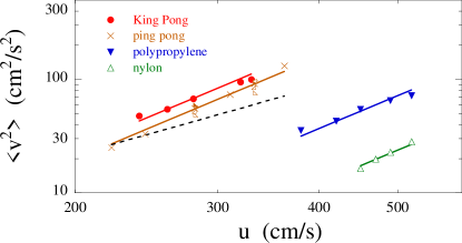
Figure 1: The mean-squared speed of a rolling sphere vs the speed of the upflow of air, for several types of sphere as labelled. The solid lines are a best fit to cubic behavior, $\langle v^{2}\rangle\sim u^{3}$. The data are not consistent with the dimensionally simpler scaling $\langle v^{2}\rangle\sim u^{2}$, shown as a dashed line. All data are for the full 12-inch sieve, except the small right triangles for ping-pong balls in cells of smaller radii.

To uncover the full scaling we first proceed by dimensional analysis. Assuming that $\langle v^{2}\rangle$ decreases with increasing sphere density, the combination $(\rho_{air}/\rho_{e})^{a}u^{3}/\langle v^{2}\rangle$ is the important characteristic speed, where the exponent $a$ of the density ratio is to be determined. We can conceive of only three possibilities for the origin of this characteristic speed: the speed of sound, 34,000 cm/s; a speed set by gravity and the sphere size, $\sqrt{gD}$; and a speed set by air viscosity and sphere size, $\eta/D$. To investigate, we compare these possibilities with data for the characteristic speed vs sphere size in Fig. 2, for several integer values of $a$. We find that the best data collapse is attained for $a=2$. For that case the value and functional form of the characteristic speed are both consistent with $\sqrt{gD}$. Adjusting the numerical prefactor to best match all the data, we thus find that the mean-squared speed of a sphere is given by

$$\langle v^{2}\rangle=0.7\left({\rho_{air}\over\rho_{e}}\right)^{2}{u^{3}\over\sqrt{gD}}.$$ (4)

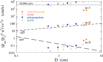
Figure 2: Scaling of the characteristics speeds with the sphere diameter, $D$, for several different spheres as labelled. The mean-squared speed $\langle v^{2}\rangle$ of the sphere is proportional to the cube of the air speed, $u^{3}$; therefore, the ratio of these quantities is a characteristic speed that reflects both the sphere density and the dissipation mechanism. The data collapse is best when $u^{3}/\langle v^{2}\rangle$ is multiplied by the square of the density ratio. Then the value and form of the characteristic speed are both consistent with $\sqrt{gD}$, indicating that rolling friction is the dominant dissipation mechanism.

This observed scaling of the mean-squared sphere speed is consistent with a simple model of the stochastic motion of the sphere being driven by turbulence in the air. The idea is to balance the rate $P_{in}$ at which kinetic energy is transferred from the air to the sphere with the rate $P_{out}$ at which energy is dissipated by drag. Ignoring numerical factors, the latter is the characteristic drag force times the characteristic sphere speed: $P_{out}=(\rho_{e}D^{3}\Gamma_{\circ}v)v$, using the notation of Section II. The former is $P_{in}=(\rho_{e}D^{3}\delta v^{2})\gamma_{\circ}$, where the term in parenthesis is the kinetic energy change due to the shedding of a wake and $\gamma_{\circ}=u/D$ is the rate at which wakes are shed. Assuming that the wake size scales with sphere size, momentum conservation gives $\rho_{e}\delta v=\rho_{air}u$. The numerical prefactor is nontrivial, since it must depend on the ratio of wake to sphere size and also on the fraction of momentum in the plane of the sieve, transverse to the average air flow direction. Combining all these elements, the balance of power input with power output is ${\rho_{air}}^{2}u^{3}/D={\rho_{e}}^{2}\langle v^{2}\rangle\Gamma_{\circ}$. This is identical to our data on the mean-squared speed, Eq. (4), provided that the drag amplitude scales as $\Gamma_{\circ}\propto\sqrt{g/D}$ and that the memory decay rate scales as $\gamma_{\circ}\propto u/D$. Next we demonstrate that these provisos both hold true.

V Drag and Random Forces

Recall from Eqs. (1-3) in Section II that both the drag and random forces are specified by an exponential memory kernal, $\Gamma(t)=\Gamma_{\circ}\gamma_{\circ}\exp(-\gamma_{\circ}t)$. In Ref. Ojha et al. (2004) we found consistent values for $\Gamma_{\circ}$ and $\gamma_{\circ}$ from two different methods. The first was from the velocity autocorrelation function using the Langevin equation. The second was from the amplitude and phase of the average response to a small sinusoidal rocking of the entire apparatus at various frequencies. Here we employ the former method for both the ping-pong and king-pong balls, as a function of air speed. The results are shown in Fig. 3, made dimensionless according to the expectations of Section IV. Specifically, the top plot demonstrates that the drag amplitude behaves as expected:

$$\Gamma_{\circ}=0.17\sqrt{g/D}.$$ (5)

The importance of $g$ suggests that rolling friction is the dominant source of drag, as opposed to shear or compression of the air. Perhaps we may identify the numerical prefactor of $g$ as a coefficient of friction, $\Gamma_{\circ}=\sqrt{\mu g/D}$ with $\mu=0.03$. It would be interesting to investigate how $\mu$ changes with mesh size and ball roughness. The bottom plot of Fig. 3 demonstrates that the memory decay rate also behaves as expected:

$$\gamma_{\circ}=0.11u/D.$$ (6)

This is consistent with earlier visualization and pressure fluctuation studies, which found that the vortex shedding frequency is $0.15u/D$ for Reynolds number in the range $10^{3}-10^{6}$ Achenbach (1974); Suryanarayana and Prabhu (2000). Here, Eq. (6) means that a new wake is shed every time the air flows a distance of about nine sphere diameters; equivalently, the Strouhal number is ${\rm St}\equiv\gamma_{\circ}D/u=0.11$.

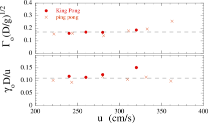
Figure 3: Amplitude $\Gamma_{\circ}$ and decay rate $\gamma_{\circ}$ of the memory kernal, $\Gamma(t)=\Gamma_{\circ}\gamma_{\circ}\exp(-\gamma_{\circ}t)$, as a function of air flow speed, for two different spheres as labelled; these quantities are rendered dimensionless by appropriate factors of sphere diameter, gravitational acceleration, and air flow speed according to expectation. The dashed lines represent average values, 0.17 in the top plot and 0.11 in the bottom plot.

We emphasize that while the results of Eqs. (5-6) directly specify the drag force, they also specify the random force via the Fluctuation-Dissipation Relation Eq. (3). The random driving and the drag forces are different aspects of the same physical interaction between the sphere and the turbulence it generates in the air. To recap, the random force has Gaussian components and an exponential temporal autocorrelation,

$$\langle{\bf F}_{r}(t^{\prime})\cdot{\bf F}_{r}(t)\rangle=2m_{e}kT\Gamma_{\circ}\gamma_{\circ}\exp[\gamma_{\circ}(t-t^{\prime})],$$ (7)

where $kT=m_{e}\langle v^{2}\rangle/2$ is specified by Eq. (4).

VI Ball-Wall Interaction

The potential $V(r)$ is the only part of the Langevin Equation not yet discussed. This can be deduced from the radial position probability function, $P(r)$, using principles of statistical mechanics. Namely, the probability to find the sphere in a thin ring of radius $r$ is proportional to the ring radius times a Boltzmann factor,

$$P(r)\propto r\exp[-V(r)/kT],$$ (8)

where $kT$ is the effective temperature discussed in Section IV. In Ref. Ojha et al. (2004), the sphere was found most frequently near the center of the cell such that the $x$ and $y$ distributions were nearly Gaussian and $P(r)\approx(2r/\langle r^{2}\rangle)\exp(-r^{2}/\langle r^{2}\rangle)$. This means that the interaction potential is nearly harmonic, $V(r)\approx Kr^{2}/2$. The value of $\langle r^{2}\rangle$ gave a spring constant that was verified by an auxiliary mechanical tilting measurement. Here, we examine the shape of the potential more closely, and we explore its behavior as a function of system parameters.

Radial position probability data for all runs are converted to the interaction potential via Eq. (8), and displayed altogether in Fig. 4. The potential is left in units of $kT$, and the radial position is scaled by the cell radius, $R_{cell}$, for clarity. Remarkably, the potential is given by the same empirical form independent of sphere size, cell radius, and air flow speed:

$$V(r)/kT={30(r/R_{cell})^{2}\over 1+(r/R_{cell})^{3}}.$$ (9)

In particular, the rms radial position of a sphere is always set by the cell size, $\sqrt{\langle r^{2}\rangle}=(0.20\pm 0.01)R_{cell}$. The harmonic form of the potential also softens away from the center. It actually becomes attractive very close to the walls, strong enough to occasionally trap an unwary sphere that wanders too far from home.

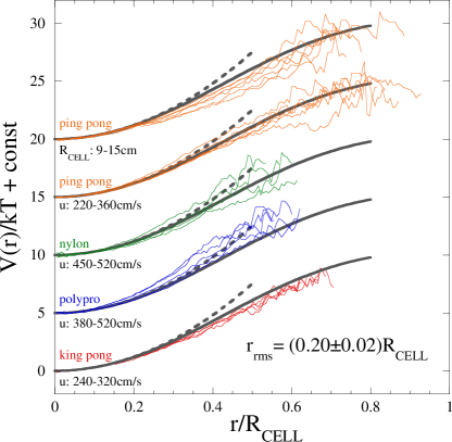
Figure 4: Interaction potential between a variety of spheres and the walls of the container, vs distance from the center of the cell scaled by cell radius. The top data set is taken at constant air flow speed, while all others are taken at constant (full) cell size. The dashed curves represent a harmonic potential, $V_{h}(r)/kT=30(r/R_{cell})^{2}$. The solid curves represent an empirical average of all the data, $V(r)/kT=30(r/R_{cell})^{2}/[1+2(r/R_{cell})^{3}]$. An arbitrary constant offset was added in order to separate the different datasets.

The geometric scaling of the potential with cell size, independent of air flow speed, leads us to believe that the origin of the behavior lies in the interaction of the shed vortices with the boundary of the cell. This is bolstered by other observations as well. First, even very slight imperfections in the circularity of the cell can break the radial symmetry of the position distributions. Second, placing a hand or other object downstream from the sphere affects its position distribution as well. Evidently, the vortex street is connected to the sphere such that force can be exerted on the sphere via perturbation to the vortices.

One possible picture for how the vortex street senses the wall is that the transverse extent of the vortices grows linearly with distance downstream. Then the sphere could sense its position from the height at which the expanding vortices hit the boundary. See Figs. 31, 55, 56, 172, and 173 of Ref. Dyke (1982) for photographs of the vortices behind various objects at approximately the same Reynolds number as here. Another possible picture is that the background flow, while homogeneous near the sieve, develops large-scale structure downstream that grows from the edge inwards. Then the sphere could senses its position from from the height at which its vortices merge with the dome of turbulent structure above. See Fig. 152-153 of Ref. Dyke (1982) for photographs of the isotropic turbulence behind a grid and it’s evolution downstream.

We performed a few tests in attempt to clarify the physical pictures. First we increased and decreased the wall height to considerable extent. This had no influence on the sphere position statistics, which seems to rule out the growing-vortex scenario. Our second test was to stretch a fine netting across the top of the sieve. We hoped that this would affect the rate of vortex shedding or the way the vortex street is connected back to the sphere. However, it had no influence on the sphere position statistics either. Thus, we must leave the origin of the geometric nature of the sphere-wall interaction potential as something of a mystery. Flow visualization may be helpful. We close by emphasizing that, whatever its origin, the sphere is repelled by the cell wall in a way that, remarkably, can be described by a potential energy and a corresponding conservative force.

VII Ball-Ball Interaction

In the remainder of this paper we report on the air-mediated interaction between two spheres rolling in the same nearly-levitating upflow of air. Throughout, we set the air flow to 280 cm/s, before adding spheres. As above, we shall see that this may be studied using position probability data and statistical mechanics. And just as for the ball-wall force, we shall see that the ball-ball force is repulsive. Naively one might expect a Bernoulli-like attraction, just as when air is blown between two objects. However it’s immediately obvious from visual inspection that here the two spheres repel. Only rarely do they collide, with physical contact between their surfaces; they never stick; they accelerate apart after close approach.

To begin we display speed and radial position probabilities in Fig. 5. The light curves are for a single ball in the same air flow, for comparison. As above and in Ref. Ojha et al. (2004), the $x$ and $y$ components of velocity and position are all Gaussian. When a second sphere is added, we verify that the velocity and position distributions remain radially symmetric and identical for each sphere. The top plot of Fig. 5 demonstrates that the average speed distribution of the two spheres remains Gaussian. Thus the mean-squared speed can be used to define an effective temperature, as before for a single sphere. However, this temperature increases when a second sphere is added, even though the flux of air remains unchanged. Evidently Eq. (4) holds in detail only for a one-sphere system. The reason may be that, due to a decrease in free area, the air flow speed around the two spheres is greater than when only one is present. It may also be that the process of energy injection via vortex shedding is altered. The bottom plot in Fig. 5 demonstrates that the radial position probability becomes non-Gaussian when a second sphere is added. Each sphere spends less time in the very center of the cell, due to mutual repulsion, with the rms radial position increasing from 2.8 cm to 4.8 cm when a second sphere is added. As before, the spheres still are repelled from the cell wall as though in a harmonic trap.

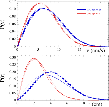
Figure 5: Speed and radial position probability functions for one and two spheres rolling in the same upflow of air. Note that the speed distributions are Gaussian in both cases, as shown by the dashed curves. By contrast, the radial position function becomes non-Gaussian when a second sphere is added to the system.

For statistical mechanics to be useful for studying the sphere-sphere repulsion, it is required that the velocity components be Gaussian as demonstrated above. It is also required that there be no correlation between the instantaneous velocities of the two spheres. To check this, we compute temporal velocity correlation functions and plot the results in Fig. 6. The velocity autocorrelation for a single sphere alone in the cell is shown by a light curve, for comparison. The velocity autocorrelation for each sphere, when two are present, is shown by a heavier curve. It decays over the same time scale as the one-sphere autocorrelation, though the oscillations are less pronounced. The cross correlation between the velocities of the two spheres is shown by a dashed curve. It too oscillates and decays over the same time scale as the autocorrelations. But, crucially for us, it vanishes at $\tau=0$. Thus the instantaneous equal-time velocities of the two spheres are indeed uncorrelated as required.

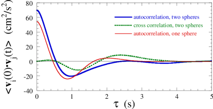
Figure 6: Velocity correlations between spheres $i$ and $j$, for one- and two-sphere systems as labelled. Note that the crosscorrelation vanishes at $\tau=0$, which is required if statistical mechanics is to be invoked.

With the above preliminaries established, we may now exploit the principles of statistical mechanics in order to deduce the sphere-sphere interaction potential $V_{ss}(\rho)$, where $\rho$ is the distance between the centers of the two spheres. The idea is to compute the sphere-sphere separation probability in terms of both the overall harmonic confining potential and the unknown $V_{ss}(\rho)$. This is accomplished by summing the Boltzmann factors for all the ways of arranging the spheres with the desired separation:

$$P(\rho) \propto \int{\rm d}x{\rm d}y{\rm d}\theta\exp\bigg{[}-{1\over 2}K\bigg{(}x^{2}+y^{2}+$$

$$(x+\rho\cos\theta)^{2}+(y+\rho\sin\theta)^{2}\bigg{)}/kT\bigg{]}$$

$$\times\exp[-V_{ss}(\rho)/kT]$$

$$\propto \exp\left[-\left({1\over 4}K\rho^{2}+V_{ss}(\rho)\right)/kT\right].$$ (11)

One may differentiate this expression to show that the peak in $P(\rho)$ is where $-{\rm d}V_{ss}/{\rm d}\rho=K\rho/2$, which is a statement of force balance when each sphere is $\rho/2$ from the center of the cell. Since the spring constant $K$ is known from the one-sphere experiment, and since the temperature $kT$ is known from the mean-squared speeds, the functions $P(\rho)$ and $V_{ss}(\rho)$ may be deduced one from the other.

The separation probability $P(\rho)$ is readily found from the video data for the position of each sphere vs time. Results are displayed by a dashed curve on the right axis of the upper plot in Fig. 7. The probability rises abruptly from zero at a separation equal to the sphere diameter. It reaches a peak near $\rho=7$ cm, and then gradually decays again toward zero. The sphere-sphere potential $V_{ss}(\rho)$ can then be obtained from $P(\rho)$ using Eq. (11). Results are shown by a solid curve on the left axis of the upper plot in Fig. 7. The precipitous drop of $V_{ss}(\rho)$ near contact indicates a hardcore repulsion. The more gradual drop at larger separations indicates a softer repulsion.

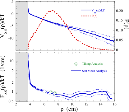
Figure 7: Interaction between two spheres as a function of their separation $\rho$. Using Eq. (11), the potential $V_{ss}(\rho)$ is inferred from the separation probability $P(\rho)$; these functions are both shown in the upper plot. Systematic uncertainty in $V_{ss}(\rho)$ is indicated by dotted curves; it is due to statistical uncertainty in the value of $K$. The repulsive force is shown in the bottom plot, as obtained both from $V_{ss}(\rho)$ and from an auxilliary mechanical measurement.

The actual force of repulsion may be found by differentiating, $F_{ss}(\rho)=-{\rm d}V_{ss}/{\rm d}\rho$. Results are shown by the solid curve in the lower plot of Fig. 7. There is a hardcore repulsion, followed by a nearly constant-force repulsion when the sphere centers are separated by more than two diameters. Expressing the interaction in terms of a force allows us to perform a check using an auxiliary mechanical measurement of the response to tilting the entire apparatus by a fixed angle $\theta$ away from horizontal. This causes a constant component of gravity, $mg\sin\theta$, within the plane and breaks the radial symmetry; note that here $m$ is the true mass, not the effective inertial mass. Then we measure the probability $\phi(x,y)$ for finding a sphere at a given position, where the origin of the coordinate system is at the center of the cell and where gravity acts in the $+\hat{y}$ direction. This probability has two peaks, at coordinates $(\pm\rho/2,y_{p})$, separated by distance $\rho$. Assuming only that the wall repulsion acts in the radial direction, the statement of force balance at the peaks of $\phi(x,y)$ gives the sphere-sphere repulsive force as

$$F_{ss}(\rho)=\left({1\over 2}\rho/y_{p}\right)mg\sin\theta.$$ (12)

In practice, to achieve a wider range in separations, we tilt the apparatus by 0.013 rad and use cells of three different diameters: 20, 25, and 30 cm. Observations then give the repulsive force at three different separations as shown in the lower plot of Fig. 7. Evidently the agreement with the results from statistical mechanics is very good. This gives confidence in the use of statistical mechanics to deduce the full form of the repulsive sphere-sphere interaction.

VIII Conclusion

We have exploited the thermal-like behavior of a single gas-fluidized sphere to deduce the nature of the forces dictating its motion. All these forces are mediated by turbulence in the gas, but can be decomposed into distinct contributions. Due to randomness in the shedding of turbulent wakes, there is a rapidly varying random force specified by Eqs.(5-7). By virtue of the Fluctuation-Dissipation Relation, and Eqs.(1-2), these results also fully specify a velocity-dependent drag force that damps rolling motion. The apparent interaction of the wakes with the cell boundary gives rise to a nearly-harmonic force that keeps the rms sphere position at about one fifth the cell radius, no matter how the system parameters are changed. The effective temperature, set by the mean-squared speed in Eq. (4), is a key parameter in these forces. When a second sphere is added, the thermal analogy still holds and these forces change only in detail. In addition, there is a gas-mediated repulsion acting between the spheres that is nearly constant beyond a few diameters of separation and that grows stronger near contact.

We thank L. Bocquet, R.F. Bruinsma, P.G. de Gennes, D. Frenkel, J.B. Freund, D. Levine, and M.A. Rutgers for useful conversations. We thank P.K. Dixon and P.-A. Lemieux for assistance with digital video techniques, and A.J. Liu for assistance with the Langevin analysis. This work was supported by NSF through grant numbers DMR-9623567 and DMR-0305106.

References

- Ruelle (2004) D. Ruelle, Phys. Today 57, 48 (2004).
- Jaeger et al. (1996) H. M. Jaeger, S. R. Nagel, and R. P. Behringer, Rev. Mod. Phys. 68, 1259 (1996).
- Duran (2000) J. Duran, Sands, powders, and grains: An introduction to the physics of granular materials, Partially ordered systems (Springer, New York, 2000).
- Bagnold (1954) R. A. Bagnold, Proc. R. Soc. London Ser. A 225, 49 (1954).
- Ogawa (1979) S. Ogawa, in Proceedings of the U.S.-Japan Symposium on Continuum Mechanics and Statistical Approaches in the Mechanics of Granular Materials, edited by S. C. Cowin and M. Satake (Gakujutsu Benken Fukyukai, Tokyo, 1979), pp. 208–217.
- Jenkins and Savage (1983) J. T. Jenkins and S. B. Savage, J. Fluid Mech. 130, 187 (1983).
- Haff (1983) P. K. Haff, J. Fluid Mech. 134, 401 (1983).
- Reydellet et al. (2000) G. Reydellet, F. Rioual, and E. Clement, Europhys. Lett. 51, 27 (2000).
- Bocquet et al. (2002) L. Bocquet, W. Losert, D. Schalk, T. C. Lubensky, and J. P. Gollub, Phys. Rev. E 65, 011307/1 (2002).
- Pouligny et al. (1990) B. Pouligny, R. Malzbender, P. Ryan, and N. A. Clark, Phys. Rev. B 42, 988 (1990).
- Ippolito et al. (1995) I. Ippolito, C. Annic, J. Lemaitre, L. Oger, and D. Bideau, Phys. Rev. E 52, 2072 (1995).
- Olafsen and Urbach (1998) J. S. Olafsen and J. S. Urbach, Phys. Rev. Lett. 81, 4369 (1998).
- Feitosa and Menon (2002) K. Feitosa and N. Menon, Phys. Rev. Lett. 88, 198301/1 (2002).
- Baxter and Olafsen (2003) G. W. Baxter and J. S. Olafsen, Nature 425, 680 (2003).
- Ojha et al. (2004) R. P. Ojha, P.-A. Lemieux, P. K. Dixon, A. J. Liu, and D. J. Durian, Nature 427, 521 (2004).
- Geldart (1986) D. Geldart, Gas fluidization technology (Wiley, New York, 1986).
- Leweke et al. (2001) T. Leweke, P. W. Bearman, and C. H. K. Williamson, Journal of Fluids & Structures 15, 377 (2001).
- Kubo et al. (1991) R. Kubo, M. Toda, and N. Hashitsume, Statistical Physics II: Nonequilibrium Statistical Mechanics (Springer-Verlag, New York, 1991), 2nd ed.
- Achenbach (1974) E. Achenbach, J. Fluid Mech. 62, 209 (1974).
- Suryanarayana and Prabhu (2000) G. K. Suryanarayana and A. Prabhu, Exp. Fluids 29, 582 (2000).
- Dyke (1982) M. V. Dyke, An Album of Fluid Motion (Parabolic Press, Stanford, 1982).