On the Nonlinear Krönig-Penney model

Abstract

We study the nonlinear Schrödinger equation with a periodic delta-function potential. This realizes a nonlinear Krönig-Penney model, with physical applications in the context of trapped Bose-Einstein condensate alkaly gases and in the transmission of signals in optical fibers. We find analytical solutions of zero-current Bloch states. Such wave-functions have the same periodicity of the potential, and, in the linear limit, reduce to the Bloch functions of the Krönig-Penney model. We also find new classes of solutions having a periodicity different from that of the external potential. We calculate the chemical potential of such states and compare it with the linear excitation spectrum.

today

Nonlinearity can deeply modify the Bloch theory of non-interacting atoms trapped in periodic potentials. Loop structures, energetic and dynamical instabilities, solitons and “generalized” Bloch states (i.e. states which do not share the same periodicity of the lattice), all arise in the context of a nonlinear Schrödinger (or Gross-Pitaevskii) equation. Applications span, for instance, the physics of dilute Bose-Einstein condensed gas trapped in optical lattices [1, 2, 3, 4, 5, 6, 7, 8, 9] or the propagation of signals in optical fibers [10]

In this paper we study analitically the nonlinear Schrödinger equation with an external Krönig-Penney (KP) potential, given by a periodic array of delta-functions. The linear Schrödinger equation with the same potential has been solved quite early in the ’30, playing a distinguished role as a model in metal’s theory [11, 12].

It is noticeable that also several properties of the nonlinear Schrödinger equation, with the same KP external potential, can be derived analitically. The most interesting results, however, are related with the emergence of new properties which do not have a counterpart in the linear case. Stationary solutions of the GPE which do not reduce to any of the eigenfunctions for a vanishing nonlinearity have been studied in [6] using a tight binding approximation, in and two-wells systems, in [13, 14, 15, 16, 17].

The mean-field model of a quasi-1D BEC trapped in a KP potential is governed by the following nonlinear Schrödinger (or Gross-Pitaevski) equation:

$$\mu\psi\left(x\right)=\left(-\frac{\hbar^{2}}{2m}\frac{\partial^{2}}{\partial x^{2}}+V\left(x\right)+g\mid\psi\left(x\right)\mid^{2}\right)\psi\left(x\right)$$ (1)

where $\mu$ is the chemical potential and $g$ the nonlinear coupling constant. The KP external potential is given by equispaced delta-functions: $V(x)=p~{}\sum^{\infty}_{n=-\infty}~{}\delta(x-na)$, having a lattice constant $a$. Since the external potential has a step-like shape, it is useful to rewrite the GPE in hydrodynamic form. With $\psi\left(x\right)=\sqrt{\rho\left(x\right)}\exp\left[-i\Theta\left(x\right)\right]$ (and in dimensionless units), we have:

$$\left({{\partial\rho}\over{\partial x}}\right)^{2}=2\eta\rho^{3}+4(\mu-V)\rho^{2}-\beta\rho-4\alpha^{2}$$ (2)

$$\Theta=\int dx{\alpha\over\rho}$$ (3)

with $\eta=gN_{0}({2ma^{2}}/\hbar^{2})$, ${x\over a}\to x$, $(\mu,V)~{}{{2ma^{2}}/\hbar^{2}}\to(\mu,V)$, $a\rho\to\rho$ and normalization $\int_{n}^{n\pm 1}dx~{}\rho(x)=1$. $N_{0}$ is the number of atoms in each well, and the integration constants $\alpha,\beta$ are fixed by the boundary conditions. In particolar, $\alpha$ has a simple physical meaning, being the current carried by the order parameter $\psi(x)$:

$$J=\alpha$$ (4)

(where $J{a^{2}\over\hbar}\to J$).

Bloch state. We derive a class of stationary solutions of Eq.s(3) having (i) the same periodicity of the external potential (Bloch states), and (ii) the linear limit: such states reduce to the well know solutions of the linear KP model when $\eta\to 0$. The Bloch theorem assures the possibility to write the complete set of eigenstates of the linear equation in the form: $\psi\left(x\right)=\exp\left(iqx\right)f_{q}\left(x\right)$, where $q$ is the quasi-momentum of the state and $f_{q}\left(x\right)$ is periodic with the lattice constant, $f_{q}\left(x+a\right)=f_{q}\left(x\right)$. It is immediate to extend the Bloch theorem and show that stationary states having the same periodicity of the potential exist also in the nonlinear case. However, there are new classes of states which do not have such properties, see next section.

Bloch nonlinear stationary states of the GPE with the KP external potential can be written in terms of the Jacobi Elliptical functions. With the same class of functions have been previously studied the exact stationary solutions of the GPE descibing a train of solitons [18], or the stationary solutions of the GPE in a double square-well potential [13, 14, 15]. To the best of our knowledge, however, the nonlinear Schrödinger equation with a periodic KP potential has not been studied so far. We notice that our results with the delta-function potential can be generalized (although becomes rather cumbersome) to a regular array of square-wells, as will been shown elsewhere.

Stationary solutions of the Eq.s(3) are:

$$\rho(x)=\frac{A}{8K^{2}}-(\frac{A}{8K^{2}}-\frac{128K^{4}\alpha^{2}}{A(16K^{4}+A\eta)})\text{SN}^{2}(Kx+\delta,n),$$ (5)

where

$$n = -\frac{A}{16K^{4}}\eta+\frac{64K^{2}\alpha^{2}}{A\left(16K^{4}+A\eta\right)}\eta$$ (6)

$$\beta = -\frac{(16K^{4}A+A^{2}\eta)^{2}+2048(A\eta+8K^{4})K^{6}\alpha^{2}}{32K^{4}(16AK^{4}+A^{2}\eta)}$$ (7)

$$\mu = K^{2}+\left(\frac{A}{8K^{2}}+\frac{64K^{4}\alpha^{2}}{A\left(16K^{4}+A\eta\right)}\right)\eta$$ (8)

and SN$\left(u,n\right)$ is the Jacobian elliptic sine function. SN$\left(u,n\right)$ has the desiderable property to give, in the linear limit, $\eta=0$, $\rho\left(x\right)=\frac{A}{8K^{2}}\cos^{2}\left(Kx+\delta\right)+8\frac{\alpha^{2}}{A}\sin^{2}\left(Kx+\delta\right)$, $\Theta(x)=\arctan(8K\alpha\tan(Kx+\delta)/A)$, which are the exact solutions of the linear KP model.

The three parameters $A$, $K$ and $\delta$ are fixed by imposing the continuity of the order parameter and the Bloch periodicity, as in the linear case. Because of the nonlinearity, however, we need one more condition to fix the chemical potential: the normalization of the density. We therefore obtain four conditions:

$$\rho_{1}\left(0\right)=\rho_{1}\left(1\right)$$ (9)

$$\partial_{x}\rho_{1}\left(0\right)-\partial_{x}\rho_{1}\left(1\right)=2P\rho_{1}\left(0\right)$$ (10)

$$\Theta_{1}\left(0\right)-\left(\Theta_{1}\left(1\right)-qt\right)=2n\pi$$ (11)

$$\int_{0}^{1}\rho_{1}\left(x\right)dx=1$$ (12)

In this paper we consider the special case of zero-current states, having $\alpha=0$ (so that $\Theta=const.$). Using the elementary properties of the Jacobian Elliptical function[19] the first two equations of (12) give:

$$\text{CN}\left(K,n\right)+\frac{P}{2K}\text{SN}\left(K,n\right)=\pm 1$$ (13)

$$n={{K^{2}-\mu}\over{2K^{2}}}$$ (14)

In the linear limit such states are at the top or at the bottom of the corresponding energy bands (which is not necessarly true in the nonlinear case when loop-like structures appear in the excitation spectrum). Indeed, the Eq.(14) with $\eta=0$ (giving $\mu=K^{2}$) reduces to the well known relation

$$\cos K+\frac{P}{2K}\sin K=\pm 1$$ (15)

giving the band and the gap widths in the linear K-P model [12].

To solve Eq.(14) we need a further relation between the chemical potential $\mu$ and $K$, provided by the normalization in (12). We obtain two conditions associated with the $+1$ and the $-1$ of Eq.(14), respectively:

$$\frac{\eta}{2K}+2{\cal E}\left(Am\left(\frac{K}{2},n\right),n\right)-\left(1-n\right)K=0~{}\text{ (+)}$$ (16)

$$\frac{\eta}{2K}+{\cal E}\left(Am\left(\varphi_{2},n\right)\right)-{\cal E}\left(Am\left(\varphi_{1},n\right)\right)+$$ (17)

$$~{}~{}~{}~{}~{}~{}~{}~{}~{}~{}~{}~{}~{}~{}~{}~{}~{}~{}~{}~{}~{}~{}~{}~{}~{}~{}~{}~{}~{}~{}~{}~{}~{}~{}~{}~{}~{}~{}~{}~{}-\left(1-n\right)K=0~{}\text{(-)}$$ (18)

where $n=\frac{1}{2}\left(1-\mu/K^{2}\right)$, $\varphi_{2}={\cal K}\left(n\right)+\frac{K}{2}$ and $\varphi_{1}={\cal K}\left(n\right)-\frac{K}{2}$. ${\cal E}\left(u,n\right)$ is the incomplete elliptic integral of the second kind and ${\cal K}$ is the complete elliptic integral of the second kind. $Am\left(\phi_{i},n\right)$ is the amplitude of $\phi_{i}$.

The coupled equations (14) and (18) can be solved graphically as shown in Fig.(1). The black lines are solutions of (14), while the color lines are solution of (18)) (the dashed and the continuum lines correspond to the $+,-$ sign, respectively). The lines among the intersections between the black and the color lines (evidenciated by the color filled regions), give the values of ($\mu,K$) corresponding to the zero-current Bloch states. As expected, nonlinearity quite modifies the lower energy bands of the systems, while, for higher bands, differences are reduced.

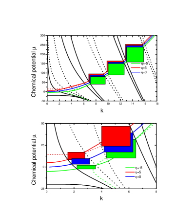
FIG. 1.: Graphical solution of the system of Eq.s(14) and Eq.s(18) for different values of nonlinearity. The allowed values of the chemical potential $\mu$ as a function of momentum $K$ are given by the intersections between the black and the color lines, in the color filled regions

Generalized Bloch states. In the previous section we have considered Bloch-like solutions, where the condensate wavefunction have the same periodicity of the potential. As already mentioned, the nonlinear interaction allows for stationary solutions which can have, in principle, any integer value period. In the following, we only consider solutions which are periodic every two sites: $f_{q}(x+2)=f_{q}(x)$. Notice that wave functions with $q=0,\pi$ are symmetric, $\psi\left(x\right)=\psi\left(x+2\right)$, while are antisymmetric when $q=\pi/2$, $\psi\left(x\right)=-\psi\left(x+2\right)$. Therefore, $f_{q=0}(x)=f_{q=\pi}(x)$, and the respective chemical potentials are equal.

In the following, we consider as elementary cell two neighboring wells separated by the delta potential, with $\rho_{l}\left(x\right)$ and $\rho_{r}\left(x\right)$ being the densities in the “left” and “right” well, respectively. As in the previous section, we consider only states with zero current $\alpha=0$. The continuity and the periodicity conditions give:

$$\rho_{l}\left(0\right)=\rho_{r}\left(2\right)$$ (19)

$$\partial_{x}\rho_{l}\left(0\right)-\partial_{x}\rho_{r}\left(2\right)=2P\rho_{l}\left(0\right)$$ (20)

$$\rho_{l}\left(1\right)=\rho_{r}\left(1\right)$$ (21)

$$\partial_{x}\rho_{r}\left(1\right)-\partial_{x}\rho_{l}\left(1\right)=2P\rho_{l}\left(1\right)$$ (22)

$$\int_{0}^{1}\rho_{l}\left(x\right)dx+\int_{1}^{2}\rho_{r}\left(x\right)dx=2$$ (23)

$$K_{1}^{2}+\frac{A_{1}}{8K_{1}^{2}}\eta-K_{2}^{2}-\frac{A_{2}}{8K_{2}^{2}}\eta=0$$ (24)

First, let’s consider the solution which have nodes at the boundary of the elementary cell:

$$\rho_{l}\left(0\right)=\rho_{r}\left(2\right)=0.$$ (25)

Then we have $\delta_{1}=\left(2l_{1}+1\right){\cal K}\left(n_{1}\right)$, $\delta_{2}+2K_{2}=\left(2l_{2}+1\right){\cal K}\left(n_{2}\right)$. Notice that the boundary conditions are equal to those of a double well, except for the condition on the first derivativies at the borders of the elementary cell, which gives $A\left(1-n_{1}\right)=B\left(1-n_{2}\right)$. Combining with the normalization, we arrive at $A=B$ and $K=Q$. Notice that this relation excludes the existence of symmetry broken solutions which are instead obtained in a single double-well potential [14]. In particolar, when $\rho_{l,r}\left(1\right)=0$, the only solutions are the Bloch states.

We now consider the case $l_{1}=l_{2}=0$, which gives:

$$-2K\text{SC}(K+{\cal K}\left(n\right))\text{DN}(K+{\cal K}\left(n\right))+P = 0$$ (26)

$$\frac{A}{8K^{2}}\int_{0}^{1}\text{CN}^{2}\left(Kx+{\cal K}\left(n\right)\right)dx = 1$$ (27)

In Fig.2, we present solutions which are symmetric with respect to the axis $x=1$. These have a linear limit, which is simply given by the superposition of two eigenfunctions having the same energy but opposite momentum. Obviously, in the nonlinear case the superposition principle breaks down, so that the existence of such solutions was not obvious.

FIG. 2.: Symmetric generalized Bloch states with no nodes (a), and with two nodes (b).

Solutions with a node in $x=1$ can be constructed from the previous conditions and imposing $\rho_{l}\left(x\right)=\rho_{r}\left(x+1\right)$, $\rho_{r}\left(x\right)=\rho_{l}\left(x-1\right)$.

There is a different class of generalized Bloch states having nodes located outside the boundaries of the potential. The conditions are:

$$\frac{A_{1}}{8K_{1}^{2}}\text{CN}^{2}\left(\delta_{1}\right)=\frac{A_{2}}{8K_{2}^{2}}\text{CN}^{2}\left(2K_{2}+\delta_{2}\right)$$ (28)

$$K_{2}\text{SC}\left(2K_{2}+\delta_{2}\right)\text{DN}\left(2K_{2}+\delta_{2}\right)+$$ (29)

$$~{}~{}~{}~{}~{}~{}~{}~{}~{}~{}~{}~{}~{}~{}-K_{1}\text{SC}\left(\delta_{1}\right)\text{DN}\left(\delta_{1}\right)=P$$ (30)

$$\frac{A_{1}}{8K_{1}^{2}}\text{CN}^{2}\left(K_{1}+\delta_{1}\right)=\frac{A_{2}}{8K_{2}^{2}}\text{CN}^{2}\left(K_{2}+\delta_{2}\right)$$ (31)

$$K_{1}\text{SC}\left(K_{1}+\delta_{1}\right)\text{DN}\left(K_{1}+\delta_{1}\right)+$$ (32)

$$~{}~{}~{}~{}~{}~{}~{}~{}~{}~{}~{}~{}~{}~{}-K_{2}\text{SC}\left(K_{2}+\delta_{2}\right)\text{DN}\left(K_{2}+\delta_{2}\right)=P$$ (33)

$$K_{1}^{2}+\frac{A_{1}}{8K_{1}^{2}}\eta-K_{2}^{2}-\frac{A_{2}}{8K_{2}^{2}}\eta=0$$ (34)

$$\frac{A_{1}}{8K_{1}^{2}}\int_{0}^{1}\text{CN}^{2}\left(K_{1}x+\delta_{1}\right)dx+$$ (35)

$$~{}~{}~{}~{}~{}~{}~{}~{}+\frac{A_{2}}{8K_{2}^{2}}\int_{1}^{2}\text{CN}^{2}\left(K_{2}x+\delta_{2}\right)dx=2$$ (36)

The density profiles of such solutions are shown in the Fig.(3), with different numbers of nodes.

FIG. 3.: Symmetry broken generalized Bloch states with three nodes (a) and with five nodes (b).

In Fig. 4 we plot the chemical potential of the system as a function of nonlinearity. The full lines corresponds to zero-current Bloch states, while the dashed and dotted lines correspond to generalized Bloch states. Notice that when $\eta\simeq-8$, the ground state ($q=0$, Bloch state) is replaced by a symmetry broken Bloch state.

FIG. 4.: Chemical potential as a function of nonlinearity

Conclusions We have studied the nonlinear Krönig-Penney model. This is given by the nonlinear Schrödinger equation with a periodic delta-function external potential. We ve found analytical solutions of zero-current states having the same (Bloch states) or a different (“generalized” Bloch states) periodicity of the potential. Nonlinear Bloch states reduce, in the linear limit, to the well known eigenfunctions of the linear Krönig-Penney model. We have studied the chemical potential dependence of such states and compared it with the linear Krönig-Penney excitation spectrum.

Acknowledgements We thanks Lev Pitaevskii for several useful discussions.

REFERENCES

- [1] J.C. Bronski, L.D. Carr, B. Deconinck, J.N. Kutz and K. Promislow, Phys. Rev. E 63 036612 (2001).
- [2] Biao Wu, Roberto B. Diener and Qian Niu, Phys. Rev. A 65 25601 (2002).
- [3] Biao Wu and Qian Niu, Phys. Rev. A 64 61603(R) (2001).
- [4] E. J. Mueller, Phys. Rev. A 66, 063603, (2002).
- [5] K. Berg-Soresen and K. Molmer, Phys. Rev. A 58, 1480, (1998).
- [6] M. Machholm, C. J. Pethick and H. Smith, Phys. Rev. A 67, 053613 (2003); M. Machholm, et al., Phys. Rev. A 69, 043604 (2004).
- [7] D. Diakonov, L. M. Jensen, C. J. Pethick and H. Smith, Phys. Rev. A 66, 013604, (2002)
- [8] M. Kramer, L. Pitaevskii and S. Stringari, Phys. Rev. Lett. 88 180404, (2002).
- [9] M. Kramer, C. Menotti, L. Pitaevskii and S. Stringari, Eur. Phys. J. D 27, 247 (2003).
- [10] See, for instance, S. Flach and C.R. Willis, Phys. Rep. 295, 182 (1998); P. G. Kevrekidis, K. . Rasmussen, A. R. Bishop, Int. J. Mod. Phys. B, 15 2833 (2001) and ref.s therein.
- [11] D.Hennig and G.P. Tsironis, Phys. Rep. 307, 333 (1999).
- [12] C. Kittel, Introduction to solid state physics, (5th edition, 1976).
- [13] K. W. Mahmud, J. N. Kutz and W. P. Reinhardt, cond-mat/0206532 (2002).
- [14] L. D. Carr, C. W. Clark and W. P. Reinhardt, Phys. Rev. A. 62, 63610 (2000), ibid, 62, 63611(2000).
- [15] L. D. Carr, K. W. Mahmud and W. P. Reinhardt, Phys. Rev. A. 64, 33603 (2000).
- [16] R. Dagosta and C. Presilla, Phys. Rev. A 65, 043609 (2002).
- [17] S. Raghavan, A. Smerzi, S. Fantoni, and S. R. Shenoy, Phys. Rev. A 59, 620 (1999).
- [18] A. V. Gurevich and A. L. Krylov, Sov. Phys. JETP 65, 5, (1987).
- [19] P. F. Byrd, M. D. Friedman, Handbook of Elliptic Integrals for Engineers and Scientists, Second. Edition, Springer-Verlage New York Heidelberg Berlin 1971.