Generalized ”Quasi-classical” Ground State for an Interacting Two Level System

We treat a system (a molecule or a solid) in which electrons are coupled linearly to any number and type of harmonic oscillators and which is further subject to external forces of arbitrary symmetry. With the treatment restricted to the lowest pair of electronic states, approximate ”vibronic” (vibration-electronic) ground state wave functions are constructed having the form of simple, closed expressions. The basis of the method is to regard electronic density operators as classical variables. It extends an earlier ”guessed solution”, devised for the dynamical Jahn-Teller effect in cubic symmetry, to situations having lower (e.g., dihedral) symmetry or without any symmetry at all. While the proposed solution is expected to be quite close to the exact one, its formal simplicity allows straightforward calculations of several interesting quantities, like energies and vibronic reduction (or Ham) factors. We calculate for dihedral symmetry two different $q$-factors (”$q_{z}$” and ”$q_{x}$”) and a $p$-factor. In simplified situations we obtain $p=q_{z}+q_{x}-1$.

The formalism enables quantitative estimates to be made for the dynamical narrowing of hyperfine lines in the observed ESR spectrum of the dihedral cyclobutane radical cation.


PACS: 71.70.Ej, 31.30.Gs, 76.30.-v

1 Historical Background and Aims

For the so called $E\otimes e$ Jahn-Teller case (involving an electron-nuclei system, in which a doubly degenerate electronic state is coupled to a doubly degenerate nuclear displacement mode) the wave function was fully obtained as long ago as 1957 [1, 2]. The physical object of reference is commonly a molecule of some high symmetry (say, one belonging to the cubic group, like $O$), or a localized impurity in a solid. The solution (or set of solutions) to this ”dynamic Jahn-Teller effect” (DJTE) are the vibronic states. Though this has received, as just noted, a full treatment early on, subsequent efforts to give simple approximate treatments or to provide additional insight into the dynamic problem have been numerous. Descriptions of some of the early works are found in two books [3, 4]. Notable are the treatments in [5]-[9]; the most recent publication known to us and involving a variational approach to this problem is in [10].

To lead us into the present work we recall a ”guessed solution” for the ground state of the linear Jahn-Teller effect, suggested by one of the present authors and collaborators, which is transparent, intuitively simple and algebraically easily manageable. This proposal was originally worked out for a molecule of cubic symmetry which had a single set of interacting normal modes [11, 12, 3]. Though not variationally obtained, the ”guessed solution” was found to have energies that are considerably closer to the exact, computed energies of [2] than other approximate solutions with which it was compared. This comparison is seen in Fig. 2 of [13]. Later treatments did not test their methods by comparison with the ”guessed solution”, though a critical review can be found in section 4.5.3 of [4].

The present work is an extension of the earlier approach to a substantially broader and harder problem, namely to a pair of electronic states in unrestricted symmetry and subject to interaction with an arbitrary number of nuclear displacement modes, but only in a linear manner. The subject of two-state interacting with bosons (which may either be phonons or photons) has had a very extensive literature. The spin-boson Hamiltonian that forms the starting point of [14] is a special case of the Hamiltonian introduced in this paper. Likewise, several books contain accounts of the related Jaynes-Cummings method [15, 16]. The present work also belongs to this field, but is restricted to a pair of ground level states. Even with this restriction, the closed solution that we present here can find its uses in treating the energy dissipation of a spin system [14].

The handling of external perturbation after taking care of the electron-nuclear interaction is a potential tool to tackle Berry phases in open systems [17, 18]. We would also recall a recent work on the Jahn-Teller effect in lower than cubic symmetry, which is less general than the present one, but has permitted us to check some of our results numerically [19]. The reduced symmetry case (named ”the elliptic form” to differentiate it from the circular energy trough in $E\otimes e$) was studied previously in [20]. We calculate (for the first time, to our knowledge) the experimentally important reduction factors for the low symmetry case (section 4.1), having pointed out (at the end of section 3.4) that, when the electron-nuclear coupling is strong, one meets broken symmetry instabilities.

The formalism, initially formulated in very general terms, is gradually shifted to more specific situations, such as systems of cubic and of lower (e.g., dihedral) symmetries, and to systems with two (rather than an arbitrary number of) vibrational modes and, ultimately, to a specific molecular system. In this last, the formalism and the numerical results for the reduction factors lead to quantitative conclusions for the dynamical narrowing of hyperfine lines in the observed ESR spectrum of the dihedral cyclobutane radical cation. This is the subject of section 5.2.

2 A General Hamiltonian

We now write down a Hamiltonian for a pair of (diabatic,  or nuclear coordinate-independent) electronic states, denoted by the symbols $\zeta_{\theta}$ and $\zeta_{\epsilon}$). The states are understood to be functions of any number of electronic coordinates, e.g, all the electrons in an atom or a molecule, but this functional dependence is absent in the formalism as long as the behavior of the doublet states alone is under consideration. A two-state situation can come about for an atom that is placed in a strongly coupled environment, such that this separates the doublet from the rest of the electronic manifold, or for a molecule in which the internal, intramolecular forces achieve the same effect. The two states need not be degenerate but, in order that it should be legitimate to consider them separately, they must be, in some sense, isolated from the rest of the electronic states (e.g, either by symmetry consideration or by a large energy gap). If so, then the ”two level-the rest” matrix elements of all interactions can be neglected to some approximation. This is the physical setting for the formalism that follows. It leads naturally to the representation of the electronic states as the column vectors

$$(\zeta_{\theta},\zeta_{\epsilon})~{}=~{}(\left(\begin{array}[]{cc}1\\ 0\end{array}\right),\left(\begin{array}[]{cc}0\\ 1\end{array}\right))$$ (1)

The electronic states are coupled to any number of nuclear displacements coordinates $q_{n}~{}(n=1,...N)$. We assume that these are organized into a set of normal modes brought to a standard form (i.e., having the same effective mass) and restrict the coupling to be of no higher order than linear in the displacement coordinates. Thus, one has for the displacement coordinates the following harmonic oscillator Hamiltonian:

$$H_{nuc}=\sum_{n=1}^{N}\frac{\hbar\omega_{n}}{2}(-\frac{\partial^{2}}{\partial q^{2}_{n}}+q^{2}_{n})$$ (2)

where $\hbar\omega_{n}$ are the quanta of vibrational energies. In the two-state representation the nuclear Hamiltonian is written as a scalar or, equivalently, as $H_{nuc}$ times the $2$x$2$ unit matrix $I$.

The remainder of the Hermitian representation matrices for the two level system are the familiar Pauli-matrices

$$\vec{\sigma}=(\sigma_{x},\sigma_{y},\sigma_{z})=(\left(\begin{array}[]{cc}0&1\\ 1&0\end{array}\right),\left(\begin{array}[]{cc}0&-i\\ i&0\end{array}\right),\left(\begin{array}[]{cc}1&0\\ 0&-1\end{array}\right))$$ (3)

In terms of these we can write out a general linear form of interaction between the electronic motion and the (real) nuclear coordinates (in the absence of any molecular symmetry), as

$$H_{el-nuc}=-\sum_{n=1}^{N}\frac{\hbar\omega_{n}}{2}(a_{n}q_{n}\sigma_{z}+b_{n}q_{n}\sigma_{x})$$ (4)

in which (the dimensionless) $a_{n}$ and $b_{n}$ express the strength of interaction between the electrons and the nuclear motion in the $n$- mode. (A detailed discussion of the linear many mode interaction in a symmetrical setting is found in section 3.5.3 of [4]. In equation (4) frequency changes between the two states are ignored to be consistent with a purely linear coupling.)

$\sigma_{y}$ is absent in the above interaction Hamiltonian, as also in several previous works [1]-[8]. When the states of the two level system are orbital states then, for all molecular point groups considered in this work, the symmetric product of the state-representations does not contain the representation of the $\sigma_{y}$-matrix. When the two states are a Kramers-doublet, the situation becomes more complex, since in a low order perturbation the coefficients $a_{n}$ and $b_{n}$ vanish, unless some further effects (like crystal field, spin-orbit interaction, external magnetic fields ${\vec{H}}$, spin-spin coupling) are included in the perturbational calculation of these coefficients. Working out the spin-lattice coupling for a Kramers’ doublet (on a six coordinated $Cu^{2+}$) Stoneham gave symmetry arguments (in the last equation of [23]) to show that, for both $a_{n}$ and $b_{n}$ to be non-zero, both $H_{x}$ and $H_{z}$ need to be non-vanishing (while $H_{y}=0$). This corresponds to the form shown in the above equation (where the coefficients would be magnetic field dependent). If, on the other hand, $H_{y}$ is also non-vanishing, then for a Kramers’ doublet a term with $\sigma_{y}$ will also be present. Since this term is absent in orbitally two-state system, we do not complicate the formalism by adding the $\sigma_{y}$ term.

One also has to consider the electron being acted upon by external fields. (The interaction of the external field on the nucleus is supposed to be contained in the potential of the nuclear coordinates.) In the preceding, vector representation of the two states, any interaction Hamiltonian (that expresses the coupling between the electron and any external field) must have the form

$$H_{el-f}=\frac{\hbar}{2}{\vec{\Omega}}\cdot\vec{\sigma}$$ (5)

with the representative of the fields ${\vec{\Omega}}=(\Omega_{x},\Omega_{y},\Omega_{z})$ inside the two level system being constant (independent of the values of the electronic or of the nuclear variables), this being the most general form of expression for the system. In section 4, which discusses the effect of external forces, we give examples for the interaction.

Any difference between the two-state energies can be considered to be part of $\Omega_{z}$ so that, until we come to the subject of the external fields in section 4, the states can be considered as a pair of degenerate doublets. However, the rest of $\Omega_{z}$ (as well as $\Omega_{x}$ and $\Omega_{y}$) comes from externally applied sources.

The total Hamiltonian $H_{tot}$ is the sum of the previous Hamiltonians

$$H_{tot}=(E_{0}+H_{nuc})I+H_{el-nuc}+H_{el-f}$$ (6)

to which has been added a scalar term with $E_{0}$ representing the mean energy of the non-interacting states. (The spin-boson Hamiltonian which forms the basis of [14] is obtained from equation (4) and equation (5) upon putting $a_{n}\neq 0$, $b_{n}=0$, $\Omega_{x}\neq 0\neq\Omega_{z}$,$\Omega_{y}=0$.)

The treatment of $H_{el-f}$ will be postponed to later. In its absence, we have a pure ”vibronic (=vibrational-electronic)” situation, which we now treat.

3 Vibronic doublet

The Hamiltonian

$$H_{v}=H_{nuc}+H_{el-nuc}$$ (7)

involving (partially) the electronic and nuclear degrees of freedom will be the subject of our investigation in this section. We first show that solutions of the partial Hamiltonian form a degenerate doublet (with the understanding that the energy difference between the two states is shifted to the external field part).

3.1 State degeneracy

The following non-identity transformation leaves the above Hamiltonian invariant:

$${\cal T}=[{\cal A}_{e}][{\cal P}_{q}]$$ (8)

where ${\cal A}_{e}$ stands for the following simultaneous changes in the electronic states $\left(\begin{array}[]{cc}1\\ 0\end{array}\right)$$\to$ $\left(\begin{array}[]{cc}0\\ -i\end{array}\right)$ and $\left(\begin{array}[]{cc}0\\ 1\end{array}\right)$ $\to$ $\left(\begin{array}[]{cc}i\\ 0\end{array}\right)$ and ${\cal P}_{q}$ is the parity operator for all mode coordinates, namely

$$P_{q}q_{n}=-q_{n}~{}~{}~{}n=1,...N$$ (9)

The transformation ${\cal A}_{e}$ can be achieved by the unitary matrix $\sigma_{y}$. But, clearly,

$${\cal T}^{2}=1$$ (10)

so that, simultaneously with any eigenvalue of the Hamiltonian $H_{v}$,  ${\cal T}$ has an eigenvalue $+1$ corresponding to a state unchanged under the ${\cal T}$-transformation and another eigenvalue $-1$, that corresponds to (another, different) state that changes sign under this transformation. The conclusion is that the vibronic Hamiltonian has doubly degenerate eigenstates. This degeneracy is lifted, when field interaction term $H_{el-f}$ is inserted, as we shall see.

3.2 The quasi-classical ground state

Based mainly on the numerical agreement of the energies under $O$ symmetry, noted in the opening section, we extend here the method of [3], [12] to the general case under study, that is, we propose the following form for the ground state wave-function

$${\hat{\Psi}}={\cal N^{\prime}}\exp\{-\frac{1}{2}\sum_{n=1}^{N}(q_{n}I-\frac{a_{n}}{2}\sigma_{z}-\frac{b_{n}}{2}\sigma_{x})^{2}\}$$ (11)

where $\cal N^{\prime}$ is a normalizing factor. The wave function generator ${\hat{\Psi}}$ is a matrix (or operator). It possesses the full ($A_{1}$) symmetry of the Hamiltonian. Therefore operating with ${\hat{\Psi}}$ on an electronic component with some symmetry, will generate a state with the symmetry of the component. In order to get the probability amplitudes in the two electronic states of equation (1) , one has to left-operate with ${\hat{\Psi}}$ on the basic vectors or on any linear combination of them, as will be shortly described. The prescription (and the underlying rationale) for the proposed construction is to regard the Pauli matrices (which are the electronic density operators) as c-numbers. Having done this, we write down the ground state wave function in the form of a set of displaced independent vibrational coordinates. The initial handling of (quantum mechanical) matrices in the manner of c-numbers has suggested naming the method ”quasi-classical”. However, the modes are now no longer independent: thus the moments (e.g., the expectation value or the spread) of any mode depends on the coupling constants of the other modes.

The mathematical meaning of the exponential form in equation (11) is that one has to expand the exponential in a power-series of the exponent. Remarkable in the posited ${\hat{\Psi}}$ is that the individual frequencies do not appear in it (just as they do not in the wave function of a set of uncoupled oscillators, when expressed in a standard form). Of course, the energy expectation value depends on the frequencies, since the Hamiltonian does and so do, implicitly, the dimensionless coupling constants $a_{n}$ and $b_{n}$.

The success of the method hinges on the fact that it is possible to sum the power series exactly, in spite of the non-commuting terms in the exponent. This is made possible by the property of the two dimensional spin (Pauli) matrices, that

$$\sigma_{i}\sigma_{j}+\sigma_{j}\sigma_{i}~{}=~{}2\delta_{ij}$$ (12)

where $\delta_{ij}$ is the Krönecker delta. Using this property, one readily obtains the simplified expression

$${\hat{\Psi}}={\cal N}[I\cosh\frac{e({\vec{q}})}{2}+\frac{\sum_{n=1}^{N}(\sigma_{z}a_{n}q_{n}+\sigma_{x}b_{n}q_{n})}{e({\vec{q}})}\sinh\frac{e({\vec{q}})}{2})]$$ (13)

with ${\cal N}$ being another normalizing factor. In the argument of the hyperbolic functions one has

$$e({\vec{q}})=\sqrt{[(\sum_{n=1}^{N}q_{n}a_{n})^{2}+(\sum_{n=1}^{N}q_{n}b_{n})^{2}]}$$ (14)

It must stressed again that the resulting quasi-classical wave-function is only an approximation, whose accuracy depends on how well the Pauli-matrices can be approximated by c-numbers. This will be the case when e.g., one of the potential wells is deep, since then the energy of the state will be dominated by the electron occupancy near the minimum. On the other hand, when the frequencies of the different oscillators differ markedly, the quasi-classical approximation could be in error, since then, e.g., the positions of the saddle points in the potential may not coincide with the maxima in the overlap of wave-functions coming from different potential wells. A scale transformation applied to each well, in the form proposed in [10, 21, 22] for cases of higher degeneracies than two and modes of various dimensionalities, could lead to improvements in the wave-function, but requires a formalism that is more complex than the one advocated here.

3.3 Some elementary symmetry considerations

As already emphasized, there need not be any relation (symmetry-based or otherwise) between the two states and among the nuclear coordinates for the foregoing formalism to hold. However, if the system has some symmetry properties (or we choose to relate it to a symmetric framework) things become at the same time clearer, more systematic and more familiar.

We therefore formulate the foregoing in a symmetry-setting and employ implicitly the theory of point molecular or point-groups.

3.3.1 Cubic symmetry

In a system which nominally belongs to a cubic symmetry group (like $O$), the two electronic states could belong to a doubly degenerate E representation, whose two components are designated in [24] as ($\theta,\epsilon$). This designation was already used by us above in equation (1) . We have chosen these symbols in preference to others, such as those in [25], because we shall later use the so-called W-coefficients and these were tabulated for the symmetry groups of interest in [24] using the present symbolism. In the expression, equation (4) , for the coupling to the nuclear motion coordinates $q_{n}$, the coefficients $a_{n}$ are non-zero for modes belonging to the $\theta$-representatives of a two-fold $e$-mode and $b_{n}$ are non-zero for modes belonging to the $\epsilon$-component of an $e$-mode, with the two coefficients being numerically pairwise equal. This is, of course, the multi-mode $E\otimes(e_{1}+e_{2}+...+e_{N/2})$ Jahn-Teller situation, described in detail in [3],[4].

${\hat{\Psi}}$ in equation (11) generates vibronic wave function in the following way. When it is let to operate on $\left(\begin{array}[]{cc}1\\ 0\end{array}\right)$, one obtains the $\theta$- component of the ground state vibronic doublet (in the present quasi-classical approximation); if it is let to operate on $\left(\begin{array}[]{cc}0\\ 1\end{array}\right)$, one obtains the $\epsilon$-component of the same. For future use we write these vibronic wave-function components in a curly ket form, as

$${\hat{\Psi}}\left(\begin{array}[]{cc}1\\ 0\end{array}\right)=|\theta\},~{}~{}~{}{\hat{\Psi}}\left(\begin{array}[]{cc}0\\ 1\end{array}\right)=|\epsilon\}$$ (15)

If, instead, one operates with ${\hat{\Psi}}$ on the two orthogonal linear combinations $\frac{1}{\sqrt{(}2)}\left(\begin{array}[]{cc}1\\ \mp 1\end{array}\right)$, one reaches a pair of other vibronic states, preferentially localized in a different part of the coordinate space than the ones in equation (15) . (These vibronic states have properties similar to polaronic states, which term is in use for a single electronic state.)

If, alternatively, one operates on the following complex combinations of the electronic states, $\frac{1}{\sqrt{(}2)}\left(\begin{array}[]{cc}1\\ \mp i\end{array}\right)$, one obtains vibronic states that have values of $+1$ and $-1$ of a ”composite” vibrational angular momenta, this being defined in terms of the composite vibrational angle variable, given by

$$\Phi=\arctan\frac{\sum_{n^{\prime}=1}^{N}b_{n^{\prime}}q_{n^{\prime}}}{\sum_{n=1}^{N}a_{n}q_{n}}$$ (16)

Clearly, although the vibrational modes were originally independent, the resulting angular variable is not the sum of the mode angular variables, like

$$\Phi=\sum_{m=1}^{\frac{N}{2}}\sum_{m^{\prime}=\frac{N}{2}+1}^{N}\arctan\frac{q_{m^{\prime}}}{q_{m}}~{}~{}~{}~{}(not~{}true)$$ (17)

This is, of course, due to the coupling of the modes to the electronic degree of freedom.

A pair of states in any of the combinations are energy-degenerate and mutually orthogonal.

3.3.2 Dihedral symmetry

In a lower symmetry situation, like $D_{2d}$, the doublet state could belong to the doubly degenerate $E$-representation, with components designated by ($\theta,\epsilon$), as before. The $a_{n}$ coefficients are non-zero for modes possessing $b_{2}$ symmetry and the $b_{n}$ coefficients belong to $b_{1}$ symmetry types. However, this time (unlike for O-symmetry) there are no symmetry-based relationships between $a$’s and $b$’s. The operator ${\hat{\Psi}}$ still possesses full ($A_{1}$) symmetry. This can best be seen in the form given in equation (13) . Here the first term is clearly invariant under all group operations (since the squares of these are the identity operator) and the second term is also invariant because it has the symmetry of the Hamiltonian. Therefore operating with ${\hat{\Psi}}$ on an electronic component with some symmetry, will again give a state with the symmetry of the component.

3.4 Energies and other expectation values in dihedral symmetry.

The advantage of the quasi-classical form is that the expectation values of c-numbers or of operators can be calculated using the explicit form of the states just given. (A recent calculation of the expectation value of an angular momentum operator is in [26].) As already noted in the opening section, these expectation values have proven to be very accurate for the single mode case in O symmetry, where comparison was made with the exact, computed results that were available. One can carry out similar calculations for several modes in any dihedral group, like one of $D_{4}$ symmetry (as well as in other dihedral groups, like $D_{4h}$, $D_{2d}$, etc). Actual results will not be given here for several modes, since these will depend on details of the system. (Some relevant molecular systems will be considered in section 5.)

A sporadic comparison has been made with results of a recent paper [19]. This paper showed graphs of eigenenergies of the (degenerate) vibronic ground computed exactly (by a numerical method), as well as with several approximation schemes. We compare the energy expectation values computed within our quasi-classical approach with theirs, at values of parameters for which the discrepancies between the exact and approximate values appear to be largest. This is the region where neither perturbation theory (weak coupling), nor asymptotic formula (very strong coupling) holds. Relating to figures 3(a) and (b) in [19] and to parameter values $a=2,b=1.5$ (equal to $\mu=0.5,\chi=0.75$ in the symbols of [19]), their exact eigenenergy is $E=-0.16725$. We compare this to $-0.15075$ obtained by our method, which is higher (as it should be for a non-exact expectation value) by $0.0165$. This discrepancy is worse than the best approximation in [19], rather better than the next best (obtained variationally) and considerably better than three others. Testing additionally our quasi-classical approximation against the exact results exhibited in the figures 4 (a) and (b) of the above reference, for $a=2\sqrt{2},b=1.5\sqrt{2}$ ($\mu=1.0,\chi=0.75$), the exact value is $E=-1.17295$, with which we can compare our value of $-1.13370$, or a discrepancy of $0.03925$. This is somewhat worse than the first and second best approximations of [19].

In summary, it seems that the intuitive, quasi-classical method can answer most practical needs for energy values. One would expect at least semi-quantitative guidance for other numerical quantities,when derived from the quasi-classical model. The next section contains some such quantities.

It is also of interest to consider the limiting case of very strong electron-vibrational coupling. This comes about when at least some of the coupling strengths $a_{n}$ and $b_{n}$ in equation (4) are numerically much larger than unity. (The opposite extreme of zero coupling has for its ”vibronic” ground states the product of gaussian states multiplying some linear combination of the electronic basic states.)

In the strong coupling limit the vibronic ground state is stabilized by the coupling and again takes the form of a product of vibrational and electronic factors. The form of the latter depends critically on the ratio of two stabilization energies. (This result goes back to Öpik and Pryce’s classic paper [29]. Modifications due to higher order coupling are treated in [30].) The stabilization energies (analogous to the static Jahn-Teller energy [3, 4]) are

$$\Delta E_{b_{2}}=\frac{1}{8}\sum_{n=1}^{N}\hbar\omega_{n}(a_{n})^{2}$$ (18)

$$\Delta E_{b_{1}}=\frac{1}{8}\sum_{n=1}^{N}\hbar\omega_{n}(b_{n})^{2}$$ (19)

where the subscripts $b_{2}$ and $b_{1}$ signify the types of the distortion mode in $D_{2d}$ symmetry. The ratio of the two

$$R=\frac{\Delta E_{b_{2}}}{\Delta E_{b_{1}}}$$ (20)

enters now so that for $R>1$ the stabilized electronic states are the $(\theta,\epsilon)$ components, shown in equation (1) , and the stabilization energy is $\Delta E_{b_{2}}$, while for $R<1$, the stabilized electronic states are $\frac{1}{\sqrt{(}2)}\left(\begin{array}[]{cc}1\\ \mp 1\end{array}\right)$ and the stabilization energy is $\Delta E_{b_{1}}$. ($R=1$ is a coincidental case in dihedral symmetry. It is the normal case under cubic symmetry and results in a continuum of stable configurations, rather than a single point in the multi-dimensional configuration space for each state.)

The transition between $R<1$ and $R>1$ represents a change from one broken symmetry type to another. The subject of broken symmetries is, of course, an important issue for macroscopic systems and also for the observed inhomogeneous state of the universe. In these cases each stabilization energy is large on a characteristic quantum scale (in a macroscopic or in an astronomical manner). Yet, it is a tiny difference between the stabilization energies that tips the balance between different types of broken symmetry. This means that if, in the neighborhood of a situation where the stabilization energies are the same, the coupling constants are made varied, then changes in the macroscopic symmetry and energy can come about by microscopic causes. (This is exemplified in our treatment of the cyclobutane radical cation in section 5.2.2.) The foregoing treatment is of course very approximate and does not take into account higher order couplings or thermal fluctuations; still, as a model it is instructive and can prove to be helpful for extensions to more realistic cases.

4 External Fields

The form of the interaction, shown in equation (5) , between the electronic part and an external field (represented by $\vec{\Omega}$) is the consequence of the Hermitian nature of the Hamiltonian, the three matrices $(\sigma_{x},\sigma_{y},\sigma_{z})$ being the only $2$x$2$ matrices having this property (apart from the unit matrix, which only shifts both states by an equal, constant amount).

4.1 Examples for ${\vec{\Omega}}$

The simplest example is the Zeeman effect on an electronic spin, for which $\vec{\Omega}=\beta{\vec{H}}$ (with $\beta$ being the Bohr magneton). The effect of a magnetic field $H_{z}$ acting within the two states ($t_{2g,\xi},t_{2g,\eta}$), which are split off from a $3d$-state manifold by crystal fields of cubic and tetragonal symmetries, would be represented by $\Omega_{y}=$constant$~{}H_{z}$, where the constant includes $\beta$ and a radial integral ([23], Table 1). A uniform stress of the type $\tau_{zz}$ acting upon a doubly degenerate set under $C_{2v}$, with $z$ the fourfold axis. will be expressed by ${\Omega_{z}}$. An applied variable electric field given by a potential $V({\vec{r}})=xyf(|{\vec{r}}|)$, when acting within an electronic pair having the real forms $|1>=xg(|{\vec{r}}|)$, $|2>=yh(|{\vec{r}}|)$ will yield

$${\Omega_{x}}=<1|V({\vec{r}})|2>$$ (21)

with all other $\Omega$-components being zero.

In a general way, for a perturbational Hamiltonian  $\Delta H$ being an arbitrary function of the coordinates, the $\Omega$- magnitudes and real and imaginary parts of the matrix elements inside the $1,2$ manifold are connected by

$$\Omega_{x}=Re(\Delta H)_{1,2},~{}~{}\Omega_{y}=-Im(\Delta H)_{1,2},~{}~{}\Omega_{z}=\frac{1}{2}((\Delta H)_{1,1}-(\Delta H)_{2,2})$$ (22)

Since the interaction term $H_{el-f}$ leads naturally to consideration of the vibronic, or Ham-, reduction factors [27, 28], we introduce these now.

4.2 Reduction factors

One starts with some coupling affecting the electrons. Within the two state manifold, this can be expressed in terms of matrix elements between these (adiabatic) states. The question is how do these matrix elements change, when the two states are no longer purely electronic, but rather vibronic (coupled electronic-vibrational) states? The answer, given in a context similar to the present one and originally due to Ham [27, 28], is a reduction in the strength of the original coupling by factors originally denoted by $q$ and $p$ (that are $1$ in the absence of vibrational coupling and less than $1$ in their presence). These reduction factors have further been described in [3] and, at considerable length, in [4] where references to several literature sources can be found. Section 4.7 in the book [4] contains an analysis of the reduction factors in terms of W-coefficients, tables for which (in both cubic and dihedral groups) can be found in [24].

In the lower symmetry situation under concern here (e.g., in dihedral symmetry), when the coupling strengths in the diagonal position differ from those in the off-diagonal positions, there are three reduction factors. These are here named $q_{x}$, $p$ and $q_{z}$. The formal definitions are in terms of the scalar product of the vibronic states introduced in equation (15) , in the form

$$q_{x}=\{\theta|\sigma_{x}|\epsilon\}=\{\epsilon|\sigma_{x}|\theta\}$$ (23)

$$q_{z}=\{\theta|\sigma_{z}|\theta\}=-\{\epsilon|\sigma_{z}|\epsilon\}$$ (24)

$$p=i\{\theta|\sigma_{y}|\epsilon\}=-i\{\epsilon|\sigma_{y}|\theta\}$$ (25)

(On notation: The subscripts of the $q$’s agree with those of the $\sigma$-matrices; the letter $p$ has been retained in preference to a possible $iq_{y}$ for historic reasons. In terms of the more recent symbols $K(a)$ used in, e.g., section 4.7.1 of [4], where $a$ is a representation of the group, one can identify:

$$q_{x}=K(B_{2})~{},~{}q_{z}=K(B_{1})~{},~{}p=K(A_{2})~{},~{}1=K(A_{1})$$ (26)

The symbol $K(a)$ will be used later in obtaining formal expressions for the reduction factors. In a higher symmetry situation (e.g. $O$) $q_{x}=q_{z}=q$, as shown on p.43 of [3], where the ket in Eq. 3.38 should be corrected to be an $\epsilon$-type.) The results of our computations are shown for the simplified situation that there is a single $b_{2}$ and a single $b_{1}$ mode coupled to the electrons. When the coupling strength are of the same strength ($a=\pm b$), our results are identical to those quoted in the literature for $O$-symmetry. In particular,

$$q_{x}=q_{z}=q,~{}~{}p=2q-1~{}~{}(in~{}O~{}symmetry)$$ (27)

but when the coupling strength are unequal a remarkable change occurs, as shown in the following figures (Fig. 1,2).

Figure 1: Reduction factors vs. dominant coupling strength $a$. The diagonal $q_{z}$ and the two off-diagonal reduction factors $q_{x}$ and $p$ are shown. Unlike the cubic-symmetry case, when $q_{x}=q_{z}$, in the dihedral case shown here the two $q$-factors are dissimilar, while $p$ remains qualitatively similar to that in cubic symmetry.

The ratio of coupling strengths $\frac{b}{a}$ is maintained a constant, $0.8$

Figure 2: Reduction factors vs. dominant coupling strength $a$. Same as figure 1, but with the ratio of coupling strengths $\frac{b}{a}$ decreased to $0.667$. The dissimilarity between $q_{z}$ and $q_{x}$ increases.

These exhibit the three reduction factors as function of increasing
strength of the dominant coupling and for two different values of the ratio $b/a$. It is apparent that while one $q$-factor decreases monotonically to zero (!), the other drops only slightly below unity and does so for only a limited range. (In cubic symmetry, also for linear coupling, the single $q$-factor decreases from unity to one-half.) The $p$-factor shows a regular behavior.

The following further results are of interest, and are capable of straightforward interpretation:

(A)  When (say) $b$ becomes very small, there is no ”reduction” in $q_{z}$, which is $\approx 1$ except in a small range of the strengths. In the limit of $b=0$ one has the simple polaron case, with no off-diagonal interaction.

(B) When (instead of the cases shown in the figure) $b>a$, the roles of the two reduction factors $q_{x}$ and $q_{z}$ are reversed.

This can be justified as follows: Interchanging $a$ and $b$ in the Hamiltonian of equation (4) has the effect of interchanging the operators $\sigma_{x}$ and $\sigma_{z}$. This interconverts, per definition in equation (23) and in equation (24) , $q_{x}$ and $q_{z}$. Formally, the interchange can be performed by applying the unitary transformation matrix $\frac{1}{\sqrt{2}}(\sigma_{x}+\sigma_{z})$ on the Hamiltonian.

(C)  The second relation in equation (27) , which is expected to hold for linear coupling to a single-mode coordinate in O symmetry, does not in general hold for neither $q$ separately, but holds accurately for their mean. Thus we find under linear $b_{1},b_{2}$ coupling in dihedral symmetries that our data satisfy the new relations

$$p=q_{x}+q_{z}-1$$ (28)

(D) Because the vibrational quanta are absent from the (proposed, quasi-classical) vibronic wave-functions, they do not play a role in the reduction factors, as long as the coupling constants are defined in the non-dimensional form, in the way done here.

4.2.1 Expressions for the reduction factors in dihedral symmetry

The following expression relates the reduction factors to the $W$-coefficients

$$W\left(\begin{array}[]{cc}a~{}b~{}c\\ d~{}e~{}f\end{array}\right)$$ (29)

defined and listed in [24] for point groups. (The definition of $W$ allows various rearrangements of the symbols, not detailed now.)

For electronic states belonging to a doublet $E$

$$K(a)=(-1)^{(a)}\lambda(E)\sum_{b}(-1)^{(b)}W\left(\begin{array}[]{cc}a~{}E~{}E\\ b~{}E~{}E\end{array}\right)<\chi_{b}^{2}>$$ (30)

In the octahedral or dihedral groups $(-1)^{(a)}$ is $-1$ for $a=A_{2}$ and $1$ otherwise. $\lambda(E)=2$ is the dimension of the $E$ representation. $<\chi_{b}^{2}>$ is the weight of the nuclear component having the $b$-representation in the vibronic state. The above formula is to be compared to the expression in Eq. (4.7.5) shown in [4], whose derivation is based on the Wigner-Eckart theorem, and to the corresponding expression for triplets in [31].

Using equation (30) and Table D3.3 in [24] one arrives at the following expressions for the reduction factor in dihedral symmetry.

$$K(A_{1})=1=<\chi_{A_{1}}^{2}>+<\chi_{A_{2}}^{2}>+<\chi_{B_{1}}^{2}>+<\chi_{B_{2}}^{2}>$$ (31)

$$K(A_{2})=p=<\chi_{A_{1}}^{2}>+<\chi_{A_{2}}^{2}>-<\chi_{B_{1}}^{2}>-<\chi_{B_{2}}^{2}>$$ (32)

$$K(B_{2})=q_{z}=<\chi_{A_{1}}^{2}>-<\chi_{A_{2}}^{2}>-<\chi_{B_{1}}^{2}>+<\chi_{B_{2}}^{2}>$$ (33)

$$K(B_{1})=q_{x}=<\chi_{A_{1}}^{2}>-<\chi_{A_{2}}^{2}>+<\chi_{B_{1}}^{2}>-<\chi_{B_{2}}^{2}>$$ (34)

$$K(E)=0$$ (35)

One notices immediately that $K(B_{2})=q_{z}\neq q_{x}=K(B_{1})$, as shown by the computed results in Figures 1 and 2. Similarly, upon adding up the first two lines and the last two lines separately and subtracting the sums from each other, one obtains

$$p-(q_{x}+q_{z}-1)=4<\chi_{A_{2}}^{2}>$$ (36)

This is similar to Eq 4.7.14 in [4] obtained in $O$ symmetry. The right hand member is non-negative. However, for what are termed in [4] ”ideal cases”, the right hand side is zero and one recaptures equation (28) , as also found in our computation. Non-ideal cases are systems with coupling to more than one pair of modes [32], and others [33, 34].

4.3 Diagonalization within the vibronic doublet

Two cases are of interest here. First, when the vibrational energies of the modes in equation (4) are finite (this excludes acoustic modes in a solid), and the external fields are weaker than the vibrational energies $|{\vec{\Omega}}|<<\omega_{n}$ (all $n$). Then the admixture by the external fields of higher vibronic states can be neglected and one can work within the ground state vibronic doublet. This is carried out here.

Secondly, when the external field components are periodic with a period $\frac{2\pi}{\omega_{f}}$ that is long, in the sense of $\omega_{f}<<|{\vec{\Omega}}|$, so that during a period the system will stay in the lowest vibronic state (the adiabatic theorem)[17, 18]. Then, again, one can work solely within a ground vibronic state . This case will be treated in a future work.

In terms of the reduction factors, the external field Hamiltonian in equation (5) changes, as follows:

$$H_{el-f}=\frac{\hbar}{2}{\vec{\Omega}}\cdot\vec{\sigma}\to\frac{\hbar}{2}{\vec{\Omega}_{v}}\cdot\vec{\sigma_{v}}=H_{v-f}$$ (37)

where

$${\vec{\Omega}_{v}}=(q_{x}\Omega_{x},p~{}\Omega_{y},q_{z}\Omega_{z})$$ (38)

and $\vec{\sigma_{v}}$ are $2$x$2$ Pauli matrices defined in the function space of the vibronic doublet.

The constant interaction Hamiltonian $H_{v-f}$ has to be diagonalized between degenerate eigenstates of $H_{v}$ in equation (7) . The diagonalization splits the states by an amount of

$$2\Delta=2\hbar|{\vec{\Omega}}_{v}|=2\hbar R_{v}$$ (39)

and selects the following two linear combinations of the $\theta$ and $\epsilon$ states:

$$|{\it l}> = -sin\frac{\theta_{v}}{2}e^{-i\frac{\phi_{v}}{2}}|\theta\}~{}+~{}cos\frac{\theta_{v}}{2}e^{i\frac{\phi_{v}}{2}}|\epsilon\}$$ (40)

$$|{\it u}> = cos\frac{\theta_{v}}{2}e^{-i\frac{\phi_{v}}{2}}|\theta\}~{}+~{}sin\frac{\theta_{v}}{2}e^{i\frac{\phi_{v}}{2}}|\epsilon\}$$ (41)

where we have defined two angles involving the three vibronic reduction factors and the three components of the field, through the expressions

$$\theta_{v}=arctan\frac{[(q_{x}~{}\Omega_{x})^{2}+(p~{}\Omega_{y})^{2}]^{\frac{1}{2}}}{q_{z}\Omega_{z}}$$ (42)

and

$$\phi_{v}=arctan\frac{p~{}\Omega_{y}}{q_{x}~{}\Omega_{x}}$$ (43)

(The reason for the notation is that ($R_{v},\theta_{v},\phi_{v}$) make up the spherical coordinate representation of the ”reduced” field vector ${\vec{\Omega}_{v}}$ in equation (38) .) $|{\it l}>$ and $|{\it u}>$ are respectively the lower and upper split states of the doublet, but for $\Omega_{z}<0$ one has to take the branch between $\frac{\pi}{2}$ and $\pi$ in the inverse tangent $\theta_{v}$.

4.3.1 A counterintuitive effect of the off-diagonal coupling on the energy splitting

For any given strength of the diagonal coupling, as the off-diagonal coupling increases, $q_{z}$ decreases. This is seen by comparing in figure 3 the three curves depicting $q_{z}$, (computed with $a>b$, so that the diagonal coupling is dominant) in which the curves decrease as the off-diagonal coupling strength increases. This behavior is unexpected for the following reason:

Figure 3: Dependence of the diagonal reduction factor $q_{z}$ on the off-diagonal coupling strength $b$. Reading the curves (here plotted against the dimensionless diagonal coupling strength $a$) from above to below, these were plotted for $b(<a)=0.2,0.5,0.8$

When $\Omega_{x}~{}=~{}\Omega_{z}~{}=~{}0$, the splitting of the vibronic doublet components is, as we have just seen in equation (39) , $2|q_{z}\Omega_{z}|$. Here $\Omega_{z}$ is a constant, while the multiplier $q_{z}$ is a function of the coupling strength parameters. However, the often quoted phenomenon known as the ”repulsion of neighboring energy levels by interaction between them” would seem to require that $q_{z}$ should grow as the off-diagonal coupling increases, so as to make the splitting wider. This does not happen, and the reason is that the off-diagonal coupling $b_{n}q_{n}$ is not just a constant (a ”magnitude”), but has a dynamical character. (We have purposely chosen for $b$ low values, to show that the result shown here is not a high-order effect in $b$. We also recall some related discussion in the literature that lay the claim that the ”repulsion between levels” need to happen only when the set of states is complete.)

5 Application to Some Low Dimensional Systems

5.1 Introductory remarks

A number of organic hydrocarbon molecules or radical ions provide instances for a doublet interacting with two independent modes. Investigations of their stereochemical properties (that is, their possible configurations) in either the ground or excited states have been lucidly summarized by Bersuker [35], giving also extensive references.

When the molecules belong to a dihedral symmetry group, they can be subject to linear couplings by two types of non-totally symmetric nuclear displacement modes. When these are of unequal strength, the adiabatic potential surface will have two minima along the dominant coordinate and two saddle points along the non-dominant one. [Couplings quadratic or of higher order in the mode coordinates (not considered in this paper and also not of paramount importance in many hydrocarbons) can turn the saddle points into minima [30].] Further distortions from these simple configurations are also possible [35, 36]. Typical energy differences between alternative configurations are of the order of 2.5 kilo-kelvins, which are also the values in these systems for the Jahn-Teller (or stabilization) energies that are relevant to the considerations in this paper.

Transitions between minima take place typically across the saddle point (a ”transition state”); this is discussed for the cyclobutane radical cation ($C_{4}H_{8}^{\cdot+}$) in [37]. (Figure 4.)

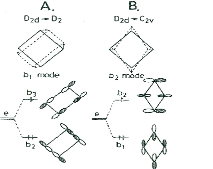
Figure 4: Distortions and states of the cyclobutane radical cation ($C_{4}H_{8}^{\cdot+}$). The upper part shows two possible distorted configurations of the frame of the four carbon atoms. Experiments favor the B configuration ($C_{2v}$). The puckered form of this configuration(two carbon atoms above the paper and two below) is not shown; neither are the positions of the eight protons (also outside the plane of the paper). The lower part shows the splitting of the energy levels of the highest lying partly occupied doubly degenerate $e$-state after distortion, as well as the shapes of the orbitals. Three spinning electrons are placed in the levels. The three-electron, product state is labelled in the text $\theta$, while the state in which $b_{2}$ is doubly occupied and $b_{1}$ singly occupied is labelled $\epsilon$. Note that the electron densities on two-two carbon atoms differ in B, but are the same in A. (With permission, after [39]. Copyright (1983) American Chemical Society.)

The activation energies for the transitions are estimated in the same source as perhaps 1 kilo-kelvin, possibly dropping below one half kilo-kelvin. With dynamic processes included, as in the present paper, the ”transition” is of course an ingredient of the ground state wave function, (also termed ”tunnelling”) and does not represent a real process. Exceptions are when the molecule is embedded in a matrix with lower symmetry than the nominal one. Then the molecule may be forced into one of the minima, from which it can make a real transition to another minima. A further instance of real transition is a thermally activated one. The two states obtained in the last section, [equation (40) , equation (41) ] can be the basis for calculating transition rates but, typically, in a thermally activated process one includes states higher than the ground doublet and their inclusion is outside our concern here.

Molecular data (like potential energy surfaces) have been calculated for the cyclobutane radical cation in [37], for the cyclobutadiene ($C_{4}H_{4}$) radical cation in [36], and for radical cations of several cycloalkanes in [38]. We cite [35] for other systems. Calculated results tend to be very sensitive to the level of the computational effort (and this sensitivity also includes the order of relative stability among different configurations). In particular, single determinant wave-functions appear to be unreliable.

Electron spin resonance (ESR) experiments have the capability of throwing light on dynamic effects, which we have studied here. Experimental determination of the vibronic reduction factors ($q_{x},p,q_{z}$) from the observed $g$-factors in the spectra are unfortunately unlikely, due to covalency effects and the small spin-orbit coupling in these cyclic compounds ( this is unlike the transition ion compounds [12, 28]). However, the behavior of the proton hyperfine lines in hydrocarbons can give a clue to dynamic processes and, especially, to their coalescence and narrowing as the temperature is raised [38, 39].

5.2 ESR in the cyclobutane radical cation

In particular, we wish to apply the present theory to the hyperfine lines of $C_{4}H_{8}^{\cdot+}$ in a solid matrix observed and discussed by the authors of [39]. Their measurement of the electron spin resonance absorption at and above $77^{0}K$ gave fairly equidistant nine-line spectra, which are indicative of electron-nuclear interaction with eight equivalent protons. On the other hand, low temperature observations at $4.2^{0}K$ showed hyperfine lines with different separations. The observed separations are consistent with non-equivalent coupling to the four pairs of protons. This non-equivalence can be understood if one has a puckered molecule in which the four carbon atoms have undergone further distortion from $D_{2d}$ to $C_{2v}$. This entails a $b_{2}$ distortion-mode leading to a rhombus-like structure, as illustrated in figure 4. In our terminology, for the coupling coefficients this implies that $|a|>|b|$.

Part of the non-equivalence among the proton pairs may well disappear at higher temperature, either by the flattening of the puckered molecule or by thermal averaging between alternative non-planar forms (assuming a softening of the barrier in the matrix at the higher temperatures). However, the remaining distinctness between two pairs of carbons (located respectively on the blunt and the sharp angle apexes of the rhombus) cannot be fitted to the high-temperature isotropic spectra. It has been suggested in [39], that the dynamic Jahn-Teller effect is capable of removing this non-equivalence.

Since the quasi-classical theory enables one to quantitatively evaluate the extent of ”democratization” of the carbon atoms, we shall now provide some numerical estimates for this.

5.2.1 Electron densities

The effects of Jahn-Teller distortions and of the motions between them on the hyperfine structure have been clearly formulated in [40, 41] and amply reviewed in [42], so that we do not have to repeat the theory. In essence, what one sees is the proton nuclear spin interacting with the electronic spin density on the carbons. For either of the carbon pairs, $C_{1}$ and $C_{3}$ on the sharp angled apexes and $C_{2}$ and $C_{4}$ on the blunt angled apexes, the spin density will differ in the $\zeta_{\theta}$ and $\zeta_{\epsilon}$ electronic states in equation (1) . The density-difference of the two states will express itself in the spectrum in an opposite manner.

On the other hand, the nuclear function cofactor of $\zeta_{\theta}$ and $\zeta_{\epsilon}$ in the vibronic state will regulate the relative weights of these electronic states in the vibronic state. We are now looking for the average weights of these electronic states. They are clearly given by the expectation values of the projection operators $P_{\theta}$ and $P_{\epsilon}$ in the vibronic state. These electronic projection operators can be written as

$$P_{\theta/\epsilon}=\frac{1}{2}(I\pm\sigma_{z})$$ (44)

Suppose now that the host matrix of the cation radical stabilizes the $\zeta_{\theta}$ electronic state in preference to the $\zeta_{\epsilon}$ state. This stabilization can come about by having the following external field parameters : $\Omega_{x}=\Omega_{y}=0$ and $\Omega_{z}=-|\Omega^{0}|<0$, leading to

$$H_{el-f}=-\frac{\hbar}{2}|\Omega^{0}|\sigma_{z}$$ (45)

(Cf. equation (5) .) In the absence of any coupling to the nuclear motion the pure electronic $\zeta_{\theta}$ state is stabilized. This state leads clearly to non-equivalent couplings, whereas equivalence is regained only for states in which $\zeta_{\theta}$ and $\zeta_{\epsilon}$ appear with equal weight.

Let us now turn on the coupling to the nuclear coordinates. By the results in section 4.2, the lower energy solution is equation (40) . Since, with our choice of the external fields, the angle $\theta_{v}=\pi$, this solution is simply the vibronic state $|\theta\}$ shown in equation (15) . We can now evaluate the expectation values of the electron projector operators in this state by using the definitions of the reduction factor $q_{z}$ in equation (24) . We get

$$\{\theta|P_{\theta}|\theta\}=\frac{1}{2}(1+q_{z})~{}~{}and~{}~{}\{\theta|P_{\epsilon}|\theta\}=\frac{1}{2}(1-q_{z})$$ (46)

What happens in the dynamic case? Remarkably, even here one does not achieve the extent of uniformity in the spin density, which is achieved in the high symmetry case (e.g., $O$) for which $q_{z}=0.5$, since, as seen in figures 1 and 2, $q_{z}$ decreases only slightly below 1, so that the difference between the two projectors will still remain. (Of course, this comes about because of the dominance of the (rhombic) $b_{2}$ distortion over the vying $b_{1}$ distortional mode.) The end-result is that under realistic conditions that the (rhombus-inducing) $b_{2}$ coupling is significantly stronger than the (rectangle-making) $b_{1}$ mode, the DJTE cannot make the two pairs of carbons equivalent, or the spectrum equidistant. For this to happen (at some elevated temperature), either the external splitting field $\Omega^{0}$ must be lowered, or fast jumps between the two vibronic eigenstates $|\theta\}$ and $|\epsilon\}$ or to higher lying vibronic states will have to occur. (”Fast” means shorter than $10^{-7}$ seconds, the hyperfine coupling time scale.)

5.2.2 Dynamic effects on hyperfine lines

A numerical estimate for the $q_{z}$-factor confirms this conclusion. We have first estimated the coupling strengths for two coupling modes in the cyclobutane radical cation from computed stabilization energies in the rectangular and rhombic configurations, shown in Figure 7 of [37]. The values obtained from the UMP2/6-31G*//UHF/6-31G* variational method were adopted, since this places the rhombic configuration below  the rectangular one, as is observed. The computed stabilization energies relative to the square configurations are $6600~{}cm^{-1}$ (for the rectangular shape) and $7250~{}cm^{-1}$ (for the rhombic form). Taking the experimental wavenumbers in cyclobutane observed by [43] for the modes: namely, $926~{}cm^{-1}$ in the $C-C$ stretching ($b_{1}$) and $1001~{}cm^{-1}$ in the $CCC$ angle bending ($b_{2}$) modes, we obtain for the dimensionless coupling strengths:

$$a_{b_{2}}=7.611,~{}~{}~{}b_{b_{1}}=7.551$$ (47)

We note that these values are close to each other.

From our expression for the vibronic wave function and a simple quadrature, we obtain for these values a reduction factor

$$q_{z}=0.999998$$ (48)

that is, near enough unity, thus excluding the attainment of equidistant spectra by a pure dynamic mechanism alone. Phrased alternatively, the relevant matrix elements of the relaxation matrix are proportional to the overlaps between Gaussian wave functions localized around different minima. These are greatly reduced by the strong vibronic coupling [44].

We recall that in $O$ symmetry, when the two coupling strengths $|a|$ and $|b|$ are precisely identical, so that $q_{z}=q_{x}=q$, for strong linear coupling these reduction factors approach $\frac{1}{2}$, which indeed halves the difference between $\theta$ and $\epsilon$ occupancies. In $D_{2d}$ symmetry, when the coupling strengths $a$ and $b$ are different and large $>>1$, the tunnelling between different stabilized wells is negligible.

6 Summary and Outlook

We have tackled (fully, though not exactly) the time-independent quantum mechanics of a pair of isolated electronic states, and this under rather general conditions: namely, the states are subject to interaction both with static external fields and with a dynamic surrounding, the latter in the linear approximation. Our non-perturbational treatment was made possible (a) by having a closed solution (the quasi-classical vibronic wave-function) for the part expressing the coupling between the electron and its dynamical surrounding, and (b) by inverting the usual order of solution through taking step (a) first and including the external field later. Thereby, the dynamically coupled states maintain convenient symmetry-group properties in the (Hilbert) function space; the external forces are subsequently treated within this framework. Their strength is, however, modified (”renormalized”) by ”vibronic” reduction factors. The use of these factors in a non-perturbational way is yet another new feature of this approach.

Branching out from the present treatment carried through for two states, one can similarly tackle problems with interactions affecting three arbitrary electronic states, as well as any chosen number of states. By extension of the approach worked out in this work and shown in equation (11) , one finds in these cases also that the wave-function generator, the generalization of $\hat{\Psi}$, is of a closed form. This consists of a finite number of terms, each with a given symmetry. Precisely, the generators (matrices) correspond to all representations of the symmetric product of the electronic multiplet in its reference group. Thus, recalling the results in this paper, for a doublet we have three matrices (those appearing in equation (13) ). (These three matrices are recognized as representatives in $O$ of the symmetric product of the E-representation, namely $A_{1}$ and $E$.) In a similar manner, for an electronic triplet one has six matrices: namely, the identity matrix, three angular momentum matrices and two more trace-less matrices. All these make up the generator wave-function. Likewise, for any larger number of states. Algebraic relations connect the functions belonging to each term, which relations have to be solved simultaneously. (The point of these remarks is to assert that the doublet is not a fluke-case, but rather a special, though by far the simplest, case of multiple electronic states in interaction with their surroundings.)

In conclusion, we restate that the major restrictions on the applicability of this work and of its possible extensions are the validity of regarding a finite number of states in isolation and the linear approximation.

7 Acknowledgments

We thank Isaac B. Bersuker, Viktor Polinger and Boris Tsukerblat for help and encouragement and Serge Shpyrko for sending us the numerical data cited in section 3.4

References

- [1] W. Moffitt and W. Thorson, Phys. Rev. 106 1251 (1957)
- [2] H.C. Longuet-Higgins, U. Öpik, M.H.L. Pryce and R.A. Sack, Proc. Roy. Soc. London A 244 1 (1958)
- [3] R. Englman, The Jahn-Teller Effect in Molecules and Crystals (Wiley, Chichester, 1972)
- [4] I.B. Bersuker and V.Z. Polinger, Vibronic Interactions in Molecules and Crystals (Springer-Verlag, Berlin, 1989)
- [5] H. Barentzen, G. Olbrich and M.C.M. O’Brien, J.Phys. A 14 111 (1981)
- [6] W.H. Wong and C.F. Lo, Phys. Lett. A 233 123 (1996)
- [7] N. Manini and E. Tosatti, Phys. Rev. B 58 782 (1998)
- [8] H. Thiel and H. Köppel, J. Chem. Phys. 110 9371 (1999)
- [9] J.E. Avron and A. Gordon, Phys. Rev. A 62 062504 (2000).
- [10] J. L. Dunn and M.R. Eccles, Phys. Rev. B 64 195 104 (2001) (and references)
- [11] R. Englman, Phys. Lett. 2 227 (1962)
- [12] R. Englman and D. Horn in Paramagnetic Resonance, editor: W. Low, Vol. I (Academic Press, New York 1963) p. 329
- [13] H. Zheng and K.-H. Bennemann, Solid State Commun. 91 213 (1994)
- [14] A.J. Leggett, S. Chakravorty, A.T. Dorsley, M.P.A. Fisher, A. Garg and W. Zwerger, Rev. Mod. Phys. 59 1 (1987)
- [15] M.O. Scully and M.S. Zubairy, Quantum Optics (University Press, Cambridge UK, 1997)
- [16] P. Meystre and M. Sargent III, Elements of Quantum Optics (Springer-Verlag, Berlin, 1999)
- [17] A. Carollo, I. Fuentes-Guridi, M Franca Santos and V. Vedral, Phys. Rev. Lett. 90 160402 (2003)
- [18] R.S. Whitney and Y. Gefen, Phys. Rev. Lett. 90 190402 (2003)
- [19] E. Majernikova and S. Shpyrko, J. Phys. (Condensed Matter) 15 2137 (2003)
- [20] M. Baer, A.M. Mebel and R. Englman, Chem. Phys. Lett. 354 243 (2002)
- [21] Y.M. Liu, C.A. Bates, J.L. Dunn and V.Z. Polinger, J. Phys. Condensed Matter 8 L523 (1996)
- [22] Y.M. Liu, J.C. Dunn, C.A. Bates and V.Z. Polinger, J. Phys. Condensed Matter 9 7119 (1997)
- [23] A. M. Stoneham, Proc. Phys. Soc. (London) 85 107 (1965)
- [24] J.S. Griffith, The Irreducible Tensor Method for Molecular Symmetry Groups (Prentice-Hall, Englewood Cliffs NJ, 1962)
- [25] G. F. Koster, J.O. Dimmock, R.G. Wheeler and H. Statz, Properties of the Thirty-two Point Groups (MIT Press, Cambridge MA, 1963)
- [26] R. Englman and A. Yahalom, Phys. Rev. A 67 054103 (2003)
- [27] F.S. Ham, Phys. Rev. 166 307 (1968)
- [28] F. S. Ham, Jahn-Teller effects in Electron Paramagnetic Resonance Spectra (Plenum, New York, 1971)
- [29] U. Öpik and M.H.L. Pryce, Proc. Roy. Soc. London A 238 425 (1957)
- [30] M. Bacci, Phys. Rev. B 17 4495 (1978)
- [31] R. Englman, M. Caner and S. Toaff, J. Phys. Soc. Japan 29 307 (1970) (Eq. (4) and following lines)
- [32] B. Halperin and R. Englman, Phys. Rev. Lett. 31 1052 (1973)
- [33] N. Gauthier, Phys. Rev. Lett. 31 (1973)
- [34] J.R. Fletcher, J. Phys. C 14 L491 (1981)
- [35] I. B. Bersuker, Chem. Rev. 101 1067 (2001) Sections II.B.2 and III.C.1
- [36] M. Roeselova, T. Bally, P. Jungwirth and P. Carsky, Chem. Phys. Lett, 234 395 (1995)
- [37] P. Jungwirth, P. Carsky and T. Bally, J. Am. Chem. Soc. 115 5776 ((1993)
- [38] K. Ohta, H. Nakatsuji, H. Kubodera and T. Shida, Chem. Phys. 76 271 (1983)
- [39] K. Ushida, T. Shida, M. Iwasaki, K. Toriyama and K. Nunome, J. Am. Chem. Soc. 105 5496 (1983)
- [40] A. D. McLachlan and L.C. Snyder, J. Chem .Phys. 36 1159 (1962)
- [41] L. C. Snyder, J. Phys. Chem. 66 22299 (1962)
- [42] L. Salem, The Molecular Orbital Theory of Conjugated Systems (Benjamin, New York, 1966)
- [43] R.C. Lord and I. Nakagawa, J. Chem. Phys. 39 2951 (1963)
- [44] V.Z. Polinger (personal communication, 2003)