Performance Variability and Project Dynamics

Abstract

We present a dynamical theory of complex cooperative projects such as large engineering design or software development efforts, comprised of concurrent and interrelated tasks. The model accounts for temporal fluctuations both in task performance and in the interactions between related tasks. We show that as the system size increases, so does the average completion time. Also, for fixed system size, the dynamics of individual project realizations can exhibit large deviations from the average when fluctuations increase past a threshold, causing long delays in completion times. This effect is in agreement with empirical observations, and can be mitigated by arranging projects in a hierarchical or modular structure.

1 Introduction

One of the main challenges in a large design project or, more generally, any problem solving process is the coordination of the different tasks comprising that project or process [15, 50, 20]. Coordination is particularly difficult in situations where the complexity of the project leads to its division into concurrent, interdependent tasks whose results must be dynamically integrated into an overall satisfactory solution. Examples are large-scale software design projects, engineering design projects, and industrial research and development efforts. It has long been recognized that because of the coupled nature of the component tasks such problem solving processes are inherently iterative in their execution [28, 53]. Information from the partial solution to a given task can trigger a chain of revisions as solutions to other, related tasks are modified [2, 8, 49, 52].

A number of formal models of cooperative processes have been proposed that predict the number of iterations required for completion, while suggesting optimal concurrency and iteration schemes which minimize the overall time or cost (e.g., [1, 18, 29, 25, 12, 42, 30, 38]). One example of these approaches is the work transformation matrix (WTM) model [43], which is an extension of the design structure matrix model (see [5] for a review). It provides a simple mathematical representation of design iterations that estimates the number of iterations and work required for a given arrangement of coupled tasks.

Helpful as these models are, they do not account for the frequent situation in which projects enter a vicious cycle of continuing revisions [10, 26, 48] resulting in budget overruns, missed business opportunities and delays which, at times, can make the final solution obsolete [4, 36, 47]. A major factor leading to these undesirable outcomes stems from the unpredictable fluctuations in the value that a particular unit of work on a single task brings to the overall project. In order to take into account these fluctuations, recent models have focused on individual sources of variability, including asynchronicity and random timing of task updates and information exchange [34, 22], information withholding [55], exogenous changes [46, 31], volatility of resource allocation [40], behavioral choice [13], uncertainty of performance evaluation [6], and the complicated landscape of performance maxima and minima [34]. However, since these models are not stochastic in nature, they do not account for the random and unpredictable nature of project dynamics, which is an intrinsic and unavoidable element of any complex cooperative project.

In this paper, we present a mathematical model of iterative problem solving processes which explicitly incorporates the fluctuating nature of task performance and interdependence. The model uses the formulation of the work transformation matrix to describe the dynamics of the project in terms of the distance to solution of the component tasks. The crucial fluctuating component is included in each updating step. Progress towards an overall solution is thus represented by a stochastic dynamic process which captures the erratic nature of the evolution of real-world projects and their component tasks. We first show that the time to solution increases on average as the number of interactions in the project increase, in agreement with empirical results [7, 17, 39, 46] and previous simulations [34, 55]. We also show that as the average strength of the fluctuations increases, the time to completion increases, also in agreement with empirical studies [24]. We demonstrate that in a large project comprising many interactive tasks, a hierarchical or modular structure can, on average, alleviate the problem of large convergence time, as previously proposed (e.g. [19]) and in agreement with empirical results [51, 44] and previous studies [33, 41, 11].

Moreover, because of the temporal variability of the fluctuations, evolution towards solution of any particular instance of a project can differ greatly from the average behavior. As a result, projects which would converge smoothly to solution in the absence of fluctuations can deviate significantly from this path. When the temporal variability is low, convergence to a solution is smooth and the finishing times are normally distributed close to the average value. But above a given threshold in variability, the distribution of finishing times undergoes a transition to a heavy-tailed log-normal form. This distribution is in agreement with earlier empirical results on cooperative problem solving [9] and implies possible finishing times far greater than the average.

Finally, we show that the effect of fluctuations is more severe in projects which converge slowly to solution. This implies that hierarchical organization not only can decrease the average time to solution, but can also mitigate the possibly unavoidable effects of fluctuating interactions.

The paper is organized as follows. In §2 we present the dynamical model and generalize it so as to take into account both synchronous and asynchronous updates of the problem solving process. In §3 we study the model’s average behavior and the relation between convergence time and project size. In §4 we consider the effects of fluctuating efforts and establish regimes that lead to large deviations away from the smooth convergence to the goal. Section 5 summarizes our results.

2 A Model of Group Problem Solving

Consider a group of individuals, or even computer programs, working cooperatively towards the solution of a problem. An example of this process in the design space is provided by a large software development effort in which individuals or teams work iteratively on pieces of the software and pass it along to others so that whole modules and eventually the whole application may be completed. Alternatively, one can conceive of teams of engineers involved in the design of a complicated mechanism that requires tight integration of all the parts in order to achieve the desired goal.

The progress of a cooperative project comprising $n$ tasks towards a solution can be represented mathematically by a state vector $\mathbf{x}$ with $n$ components, as in the WTM model of Smith and Eppinger [43]. The $i$th element of $\mathbf{x}$ represents how far task $i$ is from completion. The dynamics of the system are specified by a time-dependent interaction matrix $\mathbf{A}_{t}$ which encapsulates the interdependencies among the tasks. The state of the overall project at time $t+1$ is determined by

$$\mathbf{x}_{t+1}=\mathbf{A}_{t}\mathbf{x}_{t}$$ (1)

where $\mathbf{x}_{t}$ is the state at time $t$. The initial state $\mathbf{x}_{1}$ may be taken to be a vector of 1’s, defining the scale by which we measure how much work is left on the tasks. Ideally, as the project proceeds, the entries of the state vector will become smaller and smaller as the tasks near completion.

The interpretation of the elements of the interaction matrix is as follows (see also the example below). The off-diagonal elements measure how much one task’s partial solution helps or hinders the completion of the other tasks. A positive entry signifies that one unit of work on task $j$ causes $(A_{t})_{ij}$ units of rework on task $i$, while a zero entry means that tasks $i$ and $j$ have no direct effect on each other. In the WTM model, only positive or zero entries were allowed. Our theory allows for negative entries when efforts on task $j$’s hasten the completion of task $i$. The diagonal elements of the interaction matrix $\mathbf{A}_{t}$ account for different rates of progress on different tasks. This is in contrast to the WTM model where all tasks are performed at the same rate.

As an example, consider the following hypothetical development of an internet-based software client. The process has been divided into three modules: user interface, database front end, and network layering. It is thus modelled by a three-dimensional system as follows:

$$\mathbf{x}_{t}=\left(\begin{array}[]{c}\mbox{work remaining on user interface}\\ \mbox{work remaining on database front end}\\ \mbox{work remaining on network layering}\\ \end{array}\right)$$

The initial state $\mathbf{x}_{0}$ of the system is a vector of 1’s and the time step is one week. After a week, the state of the system is given by

$$\mathbf{x}_{2}=\mathbf{A}_{1}\mathbf{x}_{1}=\left(\begin{array}[]{ccc}0.65&0.2&0.05\\ 0.3&0.6&0.07\\ 0.09&0.05&0.7\\ \end{array}\right)\left(\begin{array}[]{c}1\\ 1\\ 1\\ \end{array}\right)=\left(\begin{array}[]{c}0.9\\ 0.97\\ 0.84\\ \end{array}\right)$$ (2)

where $\mathbf{A}_{1}$ is a hypothetical interaction matrix which describes the dynamics over the first week of the project.

Note that in this example the interdependencies between tasks slow down the overall progress. The tasks proceed rather quickly when taken alone (diagonal elements), but due to the strong interdependencies (off-diagonal elements), not much progress is made overall in the first week. The off-diagonal elements in this example were chosen to reflect the difficulties in making components of a large software effort compatible.

Project architecture

The matrices $\mathbf{A}_{t}$ entirely define the dynamics of the system by representing the interactions between tasks (off-diagonal elements) and the task work rates (diagonal elements). To a large degree, properties of the project’s architecture define the elements of the interaction matrices. Such properties include the inherent interdependence of related tasks, the structure of the organization (hierarchical, flat, etc.), and the relationships between individuals working on tasks and communities of practice [23], among others. Unless the project undergoes a major reorganization, these interactions remain constant over the project’s lifetime.

Interdependencies of this type give a constant, underlying structure to the system’s dynamics and form a basic interaction matrix $\mathbf{A}_{0}$. This matrix is simply the work transformation matrix [43], which we will refer to as the unperturbed interaction matrix or unperturbed WTM. The actual interaction matrices $\mathbf{A}_{t}$ in our model are created by introducing fluctuations into the elements of the unperturbed WTM. In practice, an unperturbed WTM can be created for a particular project by assigning numerical values to the project’s design structure matrix (DSM). The DSM is an important tool (see [5] for a review) which encapsulates a project’s interdependencies, usually by means of a survey of the individuals involved. For example, McDaniel [32] created a WTM for the appearance design of a vehicle’s interior by assigning each qualitative DSM entry a numerical value and averaging the values obtained from many sources. This process is shown in tables 1 and 2. The numerical values chosen for the interdependencies are of crucial importance to the system’s evolution, as explained in sections 3 and 4.

	1	2	3	4	5	6	7	8	9	10
1. Carpet		W	0	W	W	0	0	0	W	0
2. Center console	W		W	0	0	S	W	0	M	0
3. Door trim panel	0	W		W	0	M	0	0	M	W
4. Garnish trim	W	0	M		0	W	W	0	W	0
5. Overhead system	W	0	0	0		0	0	0	0	0
6. Instrument panel	0	S	S	W	0		W	0	0	M
7. Luggage trim	0	0	0	W	0	W		W	W	0
8. Package tray	0	0	0	W	0	0	W		M	0
9. Seats	W	M	M	W	0	W	W	M		M
10. Steering wheel	0	0	0	0	0	S	0	0	M

Table 1: Sample DSM characterizing interdependencies in appearance design of vehicle interior. Here S means strong, M medium, W weak and 0 none.

	1	2	3	4	5	6	7	8	9	10
1. Carpet	0.85	0.06	0.01	0.03	0.03	0	0	0	0.03	0
2. Center console	0.05	0.53	0.02	0	0	0.15	0.01	0	0.12	0.01
3. Door trim panel	0.01	0.02	0.47	0.04	0	0.12	0.01	0	0.09	0.01
4. Garnish trim	0.03	0	0.09	0.68	0	0.07	0.05	0.01	0.04	0
5. Overhead system	0.02	0	0	0	0.83	0	0	0	0	0
6. Instrument panel	0	0.15	0.13	0.08	0	0.28	0.03	0	0.01	0.1
7. Luggage trim	0	0.01	0.01	0.05	0	0.03	0.76	0.03	0.04	0
8. Package tray	0	0	0	0.05	0	0	0.03	0.83	0.08	0
9. Seats	0.04	0.12	0.09	0.04	0	0.02	0.02	0.08	0.63	0.1
10. Steering wheel	0	0.01	0.01	0	0	0.13	0	0	0.1	0.7

Table 2: WTM for vehicle interior appearance design process [32] created from averaging many DSM’s like the one shown in table 1. Here S interdependencies were given the value 0.15, M 0.1, and W 0.05. The diagonal elements were obtained by estimating the autonomous completion time for each component.

Fluctuations

Interactions in a cooperative problem solving process do not remain constant on short time scales but vary due to a number of features, including asynchronicity of information exchange, exogenous changes, behavioral choice, uncertainty of performance evaluation, the varying relevance of the partial solutions of related tasks to each other, and other factors as discussed in the introduction. These factors conspire to produce fluctuations in the elements of the interaction matrix. The exact nature of the fluctuations in any project is impossible to determine in advance because of the complexity of the process and of these interacting factors. The problem solving effort is thus effectively a stochastic process, where the fluctuations introduce a random component into the dynamics.

To see how these stochastic fluctuations affect the dynamics, consider the software development example introduced above. The evolution of the project in the first week was determined as shown in equation (2). During the second week, a different story unfolds, as the fluctuations alter the entries of the interaction matrix :

$$\mathbf{x}_{3}=\mathbf{A}_{2}\mathbf{x}_{2}=\left(\begin{array}[]{ccc}0.8&0.27&-0.05\\ 0.23&0.55&0.04\\ -0.03&0.02&0.7\\ \end{array}\right)\left(\begin{array}[]{c}0.9\\ 0.97\\ 0.8\\ \end{array}\right)=\left(\begin{array}[]{c}0.9419\\ 0.7725\\ 0.5524\\ \end{array}\right)$$

Note in particular that the interaction matrix has changed, so that the state vector changes in a different way from its evolution during the first week. During the second week, progress was slow on the user interface component (interaction matrix element (1,1)). Moreover, hindering interactions, perhaps due to a lack of communication with the front end developer (elements (1,2) and (2,1)), resulted in lost ground on this task. The front end itself was hurt by the bad communication but programmer 2 worked hard (element (2,2)) and made progress. The network protocol task also made good progress as its results were fortuitously compatible with those of task 1 (elements (1,3), (3,1)).

Fluctuations are reflected in our model by having the elements of the interaction matrix vary randomly in time with a given distribution. For simplicity, we assume that the distribution does not vary over the lifetime of the project. It is straightforward to relax this assumption if the project undergoes a major reorganization as explained above.

To focus on the effect of the fluctuations, we introduce new notation for the interaction matrices $\mathbf{A}_{t}$. Recall that the off-diagonal elements of $\mathbf{A}_{t}$ indicate how much one unit of work on a certain task helps or hinders a different task at time step $t$, while the diagonal elements represent the work rate on individual tasks. Consider a particular element of $\mathbf{A}_{t}$. One contribution to this element comes from the unperturbed work transformation matrix (recall the abbreviation WTM), which represents some a priori prediction of the value of the interaction. The other contribution is from the unforeseen fluctuations. This split is summarized by:

$$\mbox{\footnotesize\begin{tabular}[]{c}each element of\\ interaction matrix\end{tabular}}=\mbox{\footnotesize\begin{tabular}[]{c}unperturbed WTM\\ (constant matrix)\end{tabular}}+\mbox{\footnotesize\begin{tabular}[]{c}fluctuation part\\ (matrix which varies in time)\end{tabular}}$$

The fluctuating part of the interaction matrix is itself a matrix of random variables that vary in time with certain means and variances. For each element, the fluctuation mean indicates how far the value of the interaction is on average from the unperturbed WTM value, and the variance indicates how much temporal deviation there is from this mean. Since the fluctuation means are constant throughout the project’s lifetime, we can further split the fluctuation part as follows:

each element of interaction matrix $$= \mbox{\footnotesize\begin{tabular}[]{c}unperturbed WTM\\ (constant matrix)\end{tabular}}+\mbox{\footnotesize\begin{tabular}[]{c}fluctuation mean\\ (constant matrix)\end{tabular}}+$$

$$~{}~{}~{}~{}~{}~{}~{}~{}~{}~{}~{}~{}+\mbox{\footnotesize\begin{tabular}[]{c}varying part of fluctuation\\ (matrix of mean-zero random variables)\end{tabular}}$$

The mathematical representation of this relation is

$$\mathbf{A}_{t}=\mathbf{A}_{0}+(\mathbf{M}+\mathbf{S}_{t}),$$ (5)

where $\mathbf{A}_{0}$ is the unperturbed work transformation matrix, $\mathbf{M}$ is the matrix of mean values of the fluctuations, and $\mathbf{S}_{t}$ is a time-dependent matrix of mean-zero random variables representing the temporal variation of the fluctuations. Using this notation the dynamics of the overall problem solving process are expressed by the stochastic equation

$$\mathbf{x}_{t+1}=(\mathbf{A}_{0}+\mathbf{M}+\mathbf{S}_{t})\mathbf{x}_{t}.$$ (6)

The state vector $\mathbf{x}$ is a vector of random variables, and the dynamics of the problem solving process are characterized by the system’s average value $\langle\mathbf{x}_{t}\rangle$ and its moments $\langle|\mathbf{x}_{t}|^{p}\rangle$. The moments provide a measure of how likely the system is to be found far from its average behavior.

Stopping criterion

A final important feature of our model is the stopping criterion and the interpretation of the zero vector. We consider the zero vector to represent an “optimal” solution, and the values of the state vector as an abstract measure of the amount of work left to be done before a task’s solution is optimal. In the evolution described by equation (1), even when $\mathbf{A}_{t}$ is constant and the dynamics are convergent, the zero vector is never reached, as the state vector asymptotically approaches zero as shown in figure 1.

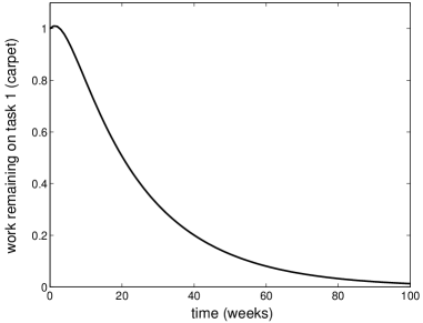
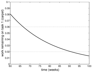
Figure 1: Simulation of project dynamics showing the evolution of the first component of the state vector. This plot was created using only the unperturbed interaction matrix $\mathbf{A}_{0}$ shown in table 2 (no fluctuations). At left, evolution over 100 weeks; at right, a plot of weeks 60–100 showing the difference in completion time for two different stopping criteria (dotted lines).

In a given project, the goal is thus reached when managers decide that the tasks’ values are close enough to zero. This is in contrast to the WTM formulation in which the zero vector must be reached for work to stop.

Our model thus implicitly contains a stopping criterion that determines when the work is finished. For example, the stopping criterion may be that all the elements of $\mathbf{x}$ are less than 0.05. Other, task-specific criteria are of course possible. As shown in the right panel of figure 1, a slight change in the stopping criterion can mean a difference of weeks or months of in the completion time. This interpretation is quite reasonable when one considers that real-world projects are always terminated by managers when the solution is deemed satisfactory by some subjective indicators.

Continuous time model

The model proposed above is discrete in time, implying that all the task states are updated at once. This is applicable to situations where individuals update their information synchronously, such as at a weekly meeting. Conversely, in situations where information is continuously passed between various individuals or subtasks in asynchronous fashion, a continuous-time model is needed [22]. In this continuum limit one obtains the stochastic differential equation [37]

$$d\mathbf{x}=[(\mathbf{A}_{0}+\mathbf{M}-\mathbf{I})dt+d\mathbf{S}(t)]\mathbf{x}(t).$$ (7)

where $d\mathbf{S}=\mathbf{S}(t)dt$ is a matrix of independent mean-zero Wiener processes with standard deviation proportional to $\sqrt{dt}$.

The introduction of fluctuations into the interaction matrix means that our model requires few assumptions about the nature of the project. The one assumption that is necessary, just as in the original WTM treatment, is that the project’s evolution can be described using a linear model. This is quite reasonable because in the early stages of a project progress on a given task is of a general nature and can be strongly interrelated to other tasks. As the project progresses and nears completion, partial solutions no longer provide much new information and the effects of a given task on others diminishes. In other words, interdependencies are stronger at earlier stages of the problem than at later ones. The mathematical expression of this weakening of the interdependencies is that the interactions are proportional to the amount of work remaining. This is a generalization of the WTM assumption that rework caused by task correlation is proportional to the work done on the previous stage.

3 Average dynamics and project size

Equations (6) and (7) describe the evolution of the cooperative solving process towards a solution. As discussed above, these equations are stochastic and describe a range of possible dynamics. In order to elucidate the possible behaviors, we first study the average dynamics of the process. As we show later, when the fluctuations in interaction strength are small, the evolution of the problem solving process is very likely to be close to the average. For larger noise, individual realizations of a given project may differ greatly from the average. Nevertheless, this quantity is important in studying the dependence on project organization, system size and interaction strengths.

As shown in appendix A, the matrices $\mathbf{S}_{t}$ do not affect the average dynamics, so the average state of the process evolves according to

$$\begin{array}[]{cclll}\langle\mathbf{x}_{t+1}\rangle&=&(\mathbf{A}_{0}+\mathbf{M})\langle\mathbf{x}_{t}\rangle&,&\mbox{discrete}\\ d\langle\mathbf{x}\rangle&=&(\mathbf{A}_{0}+\mathbf{M}-\mathbf{I})\langle\mathbf{x}(t)\rangle dt&,&\mbox{continuous}.\end{array}$$ (8)

This is a simple linear system whose dynamics are well-understood. The convergence properties are completely determined by the magnitude of the largest eigenvalue $\lambda$ of the average interaction matrix $\mathbf{A}_{0}+\mathbf{M}$. That is, if $\lambda<1$, the process will produce a satisfactory solution as the state vector $\mathbf{x}$ converges asymptotically to the zero vector; but if $\lambda>1$, the process will not yield a solution as the state vector diverges, or continues to increase. This behavior is demonstrated in figure 2.

Moreover, the value of $\lambda$ determines the rate of convergence (or divergence), with higher values of $\lambda$ implying slower convergence (or faster divergence). This property is explained below and is demonstrated in figure 2. This is the reason why the numerical values chosen to represent the qualitative entries of the DSM are so important, as demonstrated in the figure.

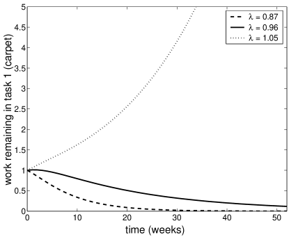
Figure 2: Simulation of average dynamics of processes with discrete dynamics and various values of $\lambda$. This plot was created using the DSM interaction matrix for the appearance design of a vehicle interior (table 1) by simply varying the numerical values assigned for strong, medium, and weak dependencies. The diagonal entries reflect the autonomous task completion rate and are those of the WTM in table 2. Here $\mathbf{M}=\mathbf{0}$.

The above convergence properties are a fundamental result of linear algebra [45] and have been noted in connection with the WTM model [43]. However, previous WTM treatments have not fully explored the elegant simplicity of this linear system, for which the asymptotic solution can be concisely expressed. To do this, we will assume that $\mathbf{A}_{0}+\mathbf{M}$ has a simple, dominant eigenvalue. Doing so we obtain (see appendix B for a derivation) the following simple expression for the long-time solution to equations (8):

$$\begin{array}[]{cclll}\langle\mathbf{x}_{t}\rangle&=&c\mathbf{u}\lambda^{t}&,&\mbox{discrete}\\ \langle\mathbf{x}(t)\rangle&=&c\mathbf{u}e^{(\lambda-1)t}&,&\mbox{continuous}\end{array}$$ (9)

where the constant $c$ is given by $c=\mathbf{v}\cdot\mathbf{x}_{0}$, and $\mathbf{u}$ and $\mathbf{v}$ are the right and left eigenvectors, respectively, of the matrix $\mathbf{A}_{0}+\mathbf{M}$ corresponding to the eigenvalue $\lambda$. Expressions (9) clearly show that the convergence rate is determined by $\lambda$. It is important to note that the long time limit may have different meanings for different systems. If the second largest eigenvalue is very small compared to $\lambda$, the above asymptotic limit may be reached very quickly, e.g. after as few as 2 or 3 iterations, as demonstrated in figure 2 above.

The dependence of the largest eigenvector on matrix properties relates the average convergence rate to parameters such as system size and organizational structure. If the organization of the problem solving process is flat, i.e., the level of interaction between all tasks is arbitrary, most of the entries of the interaction matrix are non-zero. In this case, the largest eigenvalue of $\mathbf{A}_{0}+\mathbf{M}$ is given on average by [27]

$$\lambda\sim n\mu+O(\sqrt{n}),$$ (10)

where $n$ is the size of the matrix $\mathbf{A}_{0}+\mathbf{M}$ and $\mu$ is the average value of its elements. If we further assume that the interactions are symmetric, that is, individual $i$’s results have the same effect on individual $j$ that individual $j$’s have on individual $i$, a more precise result is available [14]:

$$\lambda=n\mu+\sigma^{2}/\mu.$$ (11)

where $\sigma^{2}$ is the variance of the elements of $\mathbf{A}_{0}+\mathbf{M}$. The linear growth of $\lambda$ with the number of independent tasks ($n$) and the tendency of interactions to hinder progress ($c$) shows that the time to solution for a flat organizational structure grows quickly as the project complexity increases. The growth of $\lambda$ with $n$ is demonstrated numerically in figure 3.

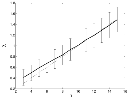
Figure 3: Largest eigenvalue of matrices of different sizes. Samples of 1000 matrices for each $n=3$ through $15$ were generated by choosing the matrix elements randomly from a distribution with average $\mu=0.15$ and standard deviation $0.3$. The solid line connects the average value of $\lambda$ for each sample, and the error bars are the standard deviations. The dotted line shows the analytic prediction $\langle\lambda\rangle\sim n\mu$.

In many situations, however, smaller teams work on parts of a problem which are then put together at a higher organizational level. From the point of view of our dynamical model, this means that each task interacts only with the other tasks of the team or their higher order aggregates. The ensuing interaction matrix will then have blocks of nonzero elements and zero entries elsewhere. In this case, a slower growth of the largest eigenvalue with size is obtained [21]:

$$\lambda\sim\mu\ln n,$$ (12)

implying that much larger groups can be stable when they are structured in highly clustered fashion, i.e. teams.

4 The effect of fluctuations

We now examine the effect of fluctuations on the dynamics of cooperative problem solving. As discussed above, these fluctuations are a key ingredient of any cooperative process and are due to many different factors. Recall that the fluctuations are included in the model by modifying the interaction matrix from the simple unperturbed WTM to the matrix $\mathbf{A}_{t}=\mathbf{A}_{0}+\mathbf{M}+\mathbf{S}_{t}$, where $\mathbf{M}$ is the matrix of the mean values of the fluctuations and $\mathbf{S}_{t}$ is a matrix of mean-zero random variables representing their temporal variation.

In the absence of fluctuations, the process is governed entirely by the unperturbed matrix $\mathbf{A}_{0}$. The dynamics are thus equivalent to the average dynamics described in section 3, with the interaction matrix $\mathbf{A}_{0}$ instead of $\mathbf{A}_{0}+\mathbf{M}$. That is, the process either converges smoothly to solution, if the largest eigenvalue of $\mathbf{A}_{0}$ is less than 1, or diverges smoothly away from solution if this eigenvalue is greater than 1. Moreover, for convergent processes, the magnitude of the largest eigenvalue of $\mathbf{A}_{0}$ determines the time to solution; processes with larger eigenvalues take longer to converge. This behavior was previously discussed and demonstrated in figure 2, above.

The fluctuations affect the dynamics of the process in two distinct ways. First, if the fluctuations have a non-zero mean, that is, they tend to help or hinder task completion, $\mathbf{M}$ is non-zero and the average dynamics are different from the unperturbed dynamics. Second, if the strength of the temporal variation $\S_{t}$ of the fluctuations exceeds a certain threshold, the dynamics of individual project realizations may deviate substantially from the smooth evolution of the average dynamics, possibly causing long delays. These two effects are explored in sections 4.1 and 4.2.

4.1 Shifted average dynamics

As mentioned above, average values of the fluctuations have the effect of shifting the average dynamics away from the unperturbed dynamics.

The unperturbed system is given by $\mathbf{x}_{t+1}=\mathbf{A}_{0}\mathbf{x}_{t}$, and the convergence rate is determined by the largest eigenvalue $\lambda_{0}$ of $\mathbf{A}_{0}$. When fluctuations are added, the average evolves according to

$$\langle\mathbf{x}_{t+1}\rangle=(\mathbf{A}_{0}+\mathbf{M})\langle\mathbf{x}_{t}\rangle$$

and the average convergence rate is shifted from $\lambda_{0}$ to $\lambda$, the largest eigenvalue of $\mathbf{A}_{0}+\mathbf{M}$. In this section for simplicity we will proceed using the discrete time formulation only; the results which follow are applicable in the continuous model as well.

Myriad forms are possible for the average fluctuation matrix $\mathbf{M}$. A reasonable form to consider is that where each element of $\mathbf{M}$ is proportional to the corresponding element of $\mathbf{A}_{0}$ by some factor $m$. That is, if the $(2,3)$ element of $\mathbf{A}_{0}$ equals 0.4, indicating a strongly hindering correlation, we would have $M_{23}=0.4m$, while for a weakly hindering element such as $(A_{0})_{12}=0.03$ we would take $M_{12}=0.03m$. This assumes that the relative strength of the correlations is not affected on average by the fluctuations. One can thus model a wide variety of behavior by varying $m$, even to have negative values. However, the most reasonable values for $m$ are positive, since unforeseen events typically hinder rather than help the completion of the project on average.

The average interaction matrix thus takes the form

$$\mathbf{A}_{0}+\mathbf{M}=(1+m)\mathbf{A}_{0}$$

and its largest eigenvalue is given simply by

$$\lambda=(1+m)\lambda_{0}.$$

This value determines the average dynamics of the perturbed system, as described in section 3. In particular, for positive values of $m$, the average effect of the fluctuations is to increase the time to solution. Moreover, if $\lambda_{0}<1$ but

$$m>\frac{1}{\lambda_{0}}-1,$$

the fluctuations cause the project to diverge on average even though an unperturbed treatment would predict convergence. This is a far more likely scenario the closer $\lambda_{0}$ is to 1, i.e., the slower the predicted convergence in the unperturbed system.

For an example, please consider the average dynamics shown in figure 2, above. The curves in this plot were generated by varying the off-diagonal entries of $\mathbf{A}_{0}$ from table 2, above, taking $\mathbf{M}=\mathbf{0}$. Note that a similar plot would be obtained by keeping $\mathbf{A}_{0}$ constant and varying $m$. Assuming that the dashed line with $\lambda=0.87$ corresponds to $m=0$, the solid line could be generated by taking $m=0.103$ and the dotted line by taking $m=0.207$. In fact, given any fluctuation in this system with $m>0.149$, the dynamics of the perturbed system will be divergent although the unperturbed system converges. Moreover, even small $m$ can cause a huge increase in convergence time as demonstrated by the dashed and solid curves in the figure.

Generally speaking, even if $\mathbf{M}$ does not take the special form studied above, a majority of positive entries in $\mathbf{M}$ indicate that the average time to solution will very likely be larger than the unperturbed prediction. It is a property of nonnegative matrices that increases to individual elements results in an increase of the largest eigenvalue [35]. Even if $\mathbf{A}_{0}$ or $\mathbf{M}$ has some negative entries, $\lambda$ will still be greater than $\lambda_{0}$ on average according to 10 if the average entry of $\mathbf{M}$ is positive.

4.2 Temporal variability

The shift in largest eigenvalue brought about by $\mathbf{M}$ and described in the previous section can engender delays in the average dynamics, which are still described by either smooth convergence to, or divergence away from, solution. Far more interesting are the deviations from this smooth path brought about by the temporal fluctuations which result in a jagged, unpredictable evolution. As we now show, a high enough level of temporal variation produces a skewed distribution of finishing times and can result in long delays.

Recall that the temporal variation of the fluctuations is represented by the matrix $\mathbf{S}_{t}$, which is a matrix of random variables with mean zero. To be as general as possible, we assume that each entry of this matrix is independent of any other. Analogously to the previous section, we also assume for definiteness that the typical size of the fluctuations is proportional to the respective average interaction values. For example, if the element $(A_{0}+M)_{35}$ = 0.1, then the standard deviation of the (3,5) element of $\mathbf{S}_{t}$ for any $t$ is equal to $0.1s$, where $s$ is a constant of proportionality. These statements can be concisely expressed by the correlation rule

$$\langle(S_{t})_{ij}(S_{t^{\prime}})_{i^{\prime}j^{\prime}}\rangle=s^{2}[(A_{0}+M)_{ij}]^{2}\delta_{tt^{\prime}}\delta_{ii^{\prime}}\delta_{jj^{\prime}},$$ (13)

where $\delta$ is the Kronecker delta.

Notice that the state of the system is determined by many random matrices multiplied together. This type of stochastic effect is known as multiplicative noise. One aspect of systems with multiplicative noise is that their distribution are approximately log-normal, with parameters proportional to time. For small fluctuations, the variance decreases with $t$ and the log-normal distribution is very similar to a normal distribution, in which events far from the average are very unlikely. However, once the fluctuations exceed a certain threshold, the variance increases with $t$ and the system’s log-normal distribution develops a heavy tail at long times, implying that events far from the average are likely.

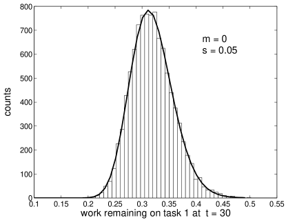
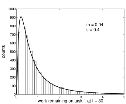
Figure 4: Histograms showing the distribution of the first component of $\mathbf{x}$ at time $t=30$ over 10,000 simulations of the vehicle interior appearance design project for various fluctuation strengths. The unperturbed WTM for this process is given in table 2. Recall the notation $m$ for the size of the fluctuation mean and $s$ for the strength of the temporal variation. The superimposed curves are log-normal probability functions calculated using the sample mean and variance and normalized by the bin width and height. The curve parameters are $\hat{\mu}=0.316,0.51,0.603$ and $\hat{\sigma}=0.123,0.486,1.019$ respectively by increasing fluctuation strength.

The log-normal character of the system is shown in figures 4 and 5, below. In figure 4, a histogram showing the work remaining on task 1 in the vehicle interior appearance design project (see tables 1 and 2, above) is shown at $t=30$ for various fluctuation strengths. Each plot’s distribution is approximately log-normal as shown in the figure by the fitted curves; note the differences in shape as the fluctuation strength increases. In figure 5, the time to solution is plotted for several levels of noise; the stopping criterion is that all components of the state vector be smaller than 0.05. This log-normal distribution of solution times is in agreement with previous results on cooperative problem solving [9].

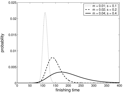
Figure 5: Distribution of finishing times for various fluctuation strengths over 10,000 simulations of the vehicle interior appearance design project. The curve parameters are $\hat{\mu}=109.9,142.61,191.07$ and $\hat{\sigma}=.0831,.179,.3238$ respectively for increasing fluctuation strength.

In order to understand the conditions under which fluctuations lead to large deviations from the average dynamics, we study the moments of the state vector. In general, the dynamics of systems whose second or third moments $\langle|\mathbf{x}_{t}|^{2}\rangle$ and $\langle|\mathbf{x}_{t}|^{3}\rangle$ are significantly larger than the powers of the average $|\langle\mathbf{x}_{t}\rangle|^{2}$ and $|\langle\mathbf{x}_{t}\rangle|^{3}$ are dominated by large deviations from the average.

In our particular case, the moments may become orders of magnitude larger than powers of the average as time goes on. This is because the moments can diverge in time even as the average converges to zero. In this situation the problem solving process is highly susceptible to long delays brought about by large deviations from the average. An example of the deviations brought about by small and large fluctuations is shown in figure 6 below.

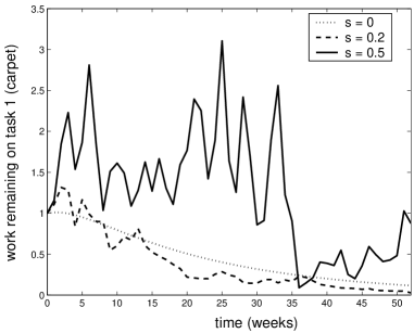
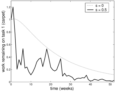
Figure 6: Example of dynamics for various fluctuation strengths. At left, the fluctuation causes a delay in task 1. At right, task 1 proceeds more quickly than an the unperturbed treatment would indicate. Recall that the parameter $s$ from (13) measures the strength of the fluctuations.

We can obtain a mathematical condition on the matrices involved which determines when the deviations described above will occur. To do this, recall expressions (9) for the evolution of the average state, which imply that powers of the average are given by

$$\begin{array}[]{lllll}|\langle\mathbf{x}_{t}\rangle|^{p}&=&c^{p}e^{tp\ln\lambda}&,&\mbox{discrete}\\ |\langle\mathbf{x}_{t}\rangle|^{p}&=&c^{p}e^{tp(\lambda-1)}&,&\mbox{continuous}.\end{array}$$ (14)

for large $t$. Here we are using the notation $\lambda$ for the largest eigenvalue of $\mathbf{A}_{0}+\mathbf{M}$ and we have normalized the right eigenvector $\mathbf{u}$ to have length 1, as is customary. In general, the moment evolution at large $t$ can also be expressed in this form:

$$\langle|\mathbf{x}_{t}|^{p}\rangle=c^{p}e^{tL_{p}}$$ (15)

(or $\langle|\mathbf{x}(t)|^{p}\rangle$ for the continuous case) where $L_{p}$ is the $p$th moment Lyapunov exponent and is always greater than the corresponding exponent in (14). The interesting case described above occurs when $\lambda<1$, so that the average dynamics are convergent, but $L_{p}>1$ for $p=2$ or 3 so that the second or third moments diverge.

The Lyapunov exponents are generally difficult to calculate. However, [54] gives a measure of the difference between the Lyapunov exponents and the corresponding exponents in the powers of the average:

$$\varepsilon^{2}=\frac{s^{2}}{\lambda^{2}}\sum_{i,j}v_{i}^{2}[(A_{0}+M)_{ij}]^{2}u_{j}^{2}.$$ (16)

Large values of $\varepsilon^{2}$ indicate that $L_{p}$ is significantly larger than $p\ln\lambda$. In this case, even a process which converges rapidly on average, i.e. with a low $\lambda$, may undergo large deviations and encounter delays. When $\varepsilon^{2}$ is small, deviations are unlikely unless the convergence of the average is very slow, i.e. $\lambda$ is close to 1. Since the variance of the $(i,j)$ element of the fluctuations is given by $s^{2}[A_{0}+M)_{ij}]^{2}$, it is clear from equation (16) that the effect of fluctuations is increased as their magnitude increases, as shown in figure 6.

To show analytically how $\varepsilon^{2}$ affects the dynamics, we consider cases in which the Lyapunov exponent in equation (15) can be approximated calculated. When the evolution is discrete and $\varepsilon^{2}$ small, the moments evolve according to [54]

$$\begin{array}[]{lllll}\langle|\mathbf{x}_{t}|^{2}\rangle&=&c^{2}e^{t(2\ln\lambda+\varepsilon^{2})}&,&\mbox{second moment}\\ \langle|\mathbf{x}_{t}|^{3}\rangle&=&c^{3}e^{t(3\ln\lambda+3\varepsilon^{2})}&,&\mbox{third moment}.\end{array}$$ (17)

These expressions show that the moments will diverge as $\varepsilon^{2}$ increases.

In the case in which the elements of the fluctuations all have the same variance $b^{2}$, [54] provides a measure of the critical strength of this variance above which deviations are likely:

$$b_{c}^{2}=\frac{1}{n+\frac{v^{2}\lambda^{2}}{1-\lambda^{2}}}.$$ (18)

When the variance of the fluctuations exceeds $b_{c}^{2}$, the second moment of the system will diverge. By applying the relation (10) we can find a corresponding critical value $s_{c}^{2}$, and thus determine the stability diagram of the project dynamics. The critical values are plotted for various $n$ in figure 7. When $\lambda<1$ but the fluctuation strength is larger than $s_{c}^{2}$ or $b_{c}^{2}$, deviations from the average are likely and although the process converges on average, significant delays are likely to occur in particular realizations of the project.

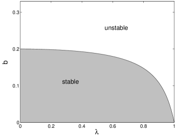
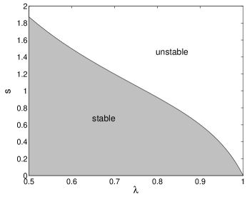
Figure 7: Stability diagram of a typical system with $n=5$. Recall that $b$ is the absolute strength of the fluctuation, while $s$ is the strength proportional to the average size of the entries of $\mathbf{A}_{0}+\mathbf{M}$.

In the continuous case, analytic results are only available for a two-dimensional system (two correlated tasks) and small noise. In this case, the moments evolve according to [3]

$$\langle|\mathbf{x}_{t}|^{p}\rangle=c^{p}\exp\big{(}t[p(\lambda-1)+p^{2}\varepsilon^{2}/2+p\gamma_{1}+pO(\varepsilon^{2})+O(p^{2})]\big{)}$$

where $\gamma_{1}$ is a complicated function of the noise and the eigenvectors $\mathbf{u}$ and $\mathbf{v}$ and $O(\varepsilon^{2})$ means an unspecified expression whose magnitude is on the order of $\varepsilon^{2}$.

5 Conclusion

In this paper we presented a dynamical theory of cooperative problem solving projects consisting of any number of interrelated tasks. The model incorporates the unavoidable fluctuating nature of the interactions in such projects, which reflect the natural variations in the amount of progress made on each task, as well as the varying relevance of information from the partial solutions of each task to any other. While simple, the theory captures key aspects of the dynamics, such as the diminishing value of interactions as the tasks near completion, as well as allowing for a satisficing decision of when the project is completed. It also captures the fact that projects with too many tasks do not converge to a desirable solution at all.

By analyzing the stochastic dynamics we showed that as the strength of the fluctuations in task effectiveness increases past a certain threshold, the convergence of a typical process to a solution is very likely to deviate from what an average treatment would indicate. In order words, single problem solving instances are likely to deviate significantly from what one would expect if fluctuations were ignored. In particular, a cooperative problem solving process may be pushed far from its goal, resulting in a significant delay in the time to solution. While this effect is most severe in problems whose average convergence is slow, large fluctuations can also disrupt the smooth convergence towards a solution in any project. This prediction is in agreement with numerous empirical results.

Moreover, over appropriate time intervals the distribution of performance among tasks is log-normally distributed, as shown in previous work on cooperative problem solving efforts. The appearance of a heavy tailed distribution above a threshold value in task variability implies that repeated observations of the evolution of a project will tend to markedly differ from the average dynamics that other models have analyzed. In other words while there might be instances where time to completion seems to be in agreement with an estimate of the average lifetime of the project, on other occasions project duration will be dramatically longer, with the concomitant aggravation of not being able to predict when such long delays will take place.

These results suggest that in order to have a predictable outcome in large cooperative projects, effort should be made to organize cooperative tasks in a way that minimizes both the instabilities implied by large unstructured groups, and the fluctuating nature of their contributions. This can be achieved by structuring tasks in such a modular or hierarchical way so that they effectively interact with very few others. Furthermore, given the stochastic nature of such processes, one possible mitigating design factor is to keep fluctuations in performance constrained to variations far below their threshold value.

Given the importance of large teams in the design and solution of technical problems and the increasing need for production agility, the study of the dynamics of group problem solving offers new insights into the organization of teams and their efficiency at solving complex tasks.

Acknowledgement

This work was partially supported by the National Science Foundation under Grant No. 9986651

Appendices

Appendix A Fluctuations have no effect on the average

As mentioned above, the average dynamics of the system are not affected by the fluctuations. In order to see this, notice that in the discrete case the system evolves according to $\mathbf{x}_{t}=(\mathbf{C}+\mathbf{B}_{t})\mathbf{x}_{t-1}$. Since the fluctuations are Markovian, i.e. the components of the matrix $B_{t}$ are independent of the state at previous times,

$$\langle\mathbf{x}_{t}\rangle=[\mathbf{C}+\langle\mathbf{B}_{t}\rangle]\langle\mathbf{x}_{t-1}\rangle$$

and we are taking the expected value of $\mathbf{B}_{t}$ entry by entry, $\langle(B_{\tau})_{ij}\rangle=0$ for all $\tau$, $i$ and $j$, we have $\langle\mathbf{x}_{t}\rangle=\mathbf{C}\langle\mathbf{x}_{t-1}\rangle$ and, extrapolating back to $t=0$, we obtain the discrete version of equation (8). Similarly, in the continuous case formal integration gives

$$\mathbf{x}(t)=\int_{0}^{t}(\mathbf{C}-\mathbf{I})\mathbf{x}(s)ds+\int_{0}^{t}d\mathbf{W}\mathbf{x}(s).$$

Since $d\mathbf{W}=\mathbf{B}(t)dt$ and the elements of $\mathbf{B}$ have mean 0,

$$\left\langle\int d\mathbf{W}\mbox{\boldmath$\phi$}(\mathbf{x},s)\right\rangle=0$$

for any function $\mbox{\boldmath$\phi$}(\mathbf{x},s)$ and the expected value is given simply by

$$\langle\mathbf{x}(t)\rangle=\int_{0}^{t}(\mathbf{A}-\mathbf{I})\langle\mathbf{x}(s)\rangle ds,$$

which is equivalent to the continuous version of equation (8).

Appendix B Dynamics of a simple linear system

For any dynamical system specified by the equations

$$\begin{array}[]{cclll}\langle\mathbf{x}_{t+1}\rangle&=&\mathbf{C}\langle\mathbf{x}_{t}\rangle&,&\mbox{discrete}\\ d\langle\mathbf{x}\rangle&=&\mathbf{C}\langle\mathbf{x}(t)\rangle dt&,&\mbox{continuous}\end{array}$$

the state at any time may be expressed in terms of the initial state by writing

$$\begin{array}[]{cclll}\langle\mathbf{x}_{t}\rangle&=&\mathbf{C}^{t}\mathbf{x}_{0}&,&\mbox{discrete}\\ \langle\mathbf{x}(t)\rangle&=&e^{(\mathbf{C}-\mathbf{I})t}\mathbf{x}(0)&,&\mbox{continuous}.\end{array}$$ (19)

In the long time limit, the matrix product $\mathbf{C}^{t}$ and the matrix exponential $e^{(\mathbf{C}-\mathbf{I})t}$ in these equations are dominated by the contribution from the largest eigenvalue for large $t$. To see this, we diagonalize $\mathbf{C}$ into the form $\mathbf{C}=\mathbf{P}\mbox{\boldmath$\Lambda$}\mathbf{P}^{-1}$, where $\Lambda$ is the diagonal matrix of eigenvalues of $\mathbf{C}$. This simplifies equations (19) because

$$\mathbf{C}^{t} = \mathbf{P}\mbox{\boldmath$\Lambda$}^{t}\mathbf{P}^{-1}$$

$$= \mathbf{P}\left(\begin{array}[]{cccc}\lambda_{1}^{t}&&&\\ &\lambda_{2}^{t}&&\\ &&\ddots&\\ &&&\lambda_{n}^{t}\end{array}\right)\mathbf{P}^{-1},$$

where the $\{\lambda_{i}\}$ are the eigenvalues of $\mathbf{C}$, and

$$e^{(\mathbf{C}-\mathbf{I})t} = \mathbf{P}e^{{\mbox{{\scriptsize\boldmath$\Lambda$}}}-\mathbf{I}t}\mathbf{P}^{-1}$$

$$= \mathbf{P}\left(\begin{array}[]{cccc}e^{(\lambda_{1}-1)t}&&&\\ &e^{(\lambda_{2}-1)t}&&\\ &&\ddots&\\ &&&e^{(\lambda_{n}-1)t}\end{array}\right)\mathbf{P}^{-1}.$$

Since $\lambda$ is the largest eigenvalue, when $t$ is large $\lambda^{t}$ and $e^{(\lambda-1)t}$ are much, much greater than all other terms in the above matrices. The above equations are thus dominated by $\lambda$ and its eigenvectors $\mathbf{u}$ (corresponding column of $\mathbf{P}$) and $\mathbf{v}$ (corresponding row of $\mathbf{P}^{-1}$). Expanding the matrix product with all entries of $\Lambda$ neglected except the ones with $\lambda$, we obtain (9).

Appendix C Log-normal distribution

The log-normal probability distribution describes a random variable whose logarithm is normally distributed. The probability density function is

$$P(x)=\frac{1}{x\sigma\sqrt{2\pi}}e^{\frac{(\ln x-\ln\mu)^{2}}{2\sigma^{2}}}$$ (22)

where $\mu$ and $\sigma$ are the mean and standard deviation of the normal distribution that describes $\ln x$. The $p$th moment of the log-normal distribution is given by

$$\langle x^{p}\rangle=\exp\big{(}p\ln\mu+\frac{p^{2}\sigma^{2}}{2}\big{)}.$$ (23)

In our application, $\sigma^{2}$ and $\ln\mu$ are proportional to $t$. For large $\sigma^{2}$ the moments diverge for large enough $p$, causing large deviations from the average.

References

- [1] R. H. Ahmadi and H. Wang, Rationalizing product design development processes, (1994). UCLA Anderson Graduate School of Management Working Paper.
- [2] T. J. Allen, Studies of the problem-solving process in engineering, IEEE Trans. Engrg. Management, EM-13 (1966), pp. 72–83.
- [3] L. Arnold, M. M. Doyle, and N. S. Namachchivaya, Small noise expansion of moment Lyapunov exponents for two-dimensional systems, Dynamics and Stability of Systems, 12 (1997), pp. 187–211.
- [4] F. Brooks, The Mythical Man-month, Addison-Wesley, Reading, Mass., 1975.
- [5] T. Browning, Applying the design structure matrix to system decomposition and integration problems: a review and new directions, IEEE Trans. Eng. Management, 48 (2001), pp. 292–306.
- [6] T. Browning, J. Deyst, S. D. Eppinger, and D. Whitney, Adding value in product development by creating information and reducing risk, IEEE Trans Engrg Management, 49 (2002), pp. 428–442.
- [7] K. B. Clark, Project scope and project performance: the effect of parts strategy and supplier involvement on product development, Management Sci., 35 (1989), pp. 1247–1263.
- [8] K. B. Clark and T. Fujimoto, Product Development Performance: Strategy, Organization, and Management in the World Auto Industry, Harvard Business School Press, Boston, 1991.
- [9] S. Clearwater, B. Huberman, and T. Hogg, Cooperative solution of constraint satisfaction problems, Science, 254 (1991), pp. 1181–1183.
- [10] M. Cusumano and R. Selby, Microsoft Secrets, Free Press, New York, 1995.
- [11] S. K. Ethiraj and D. Levinthal, Modularity and innovation in complex systems, Management Sci., 50 (2004), pp. 159–173.
- [12] D. Ford and J. Sterman, Dynamic modeling of product development processes, System Dynamics Review, 14 (1998), pp. 31–68.
- [13] , Overcoming the 90 percent syndrome: interation management in concurrent development projects, (1999). Working paper, Texas A&M University.
- [14] Z. Füredi and J. Komlós, The eigenvalues of random symmetric matrices, Combinatorica, 1 (1981), pp. 233–241.
- [15] J. R. Galbraith, Organizational Design, Addison-Wesley, Reading, Mass., 1977.
- [16] G. H. Golub and C. F. van Loan, Matrix Computations, The Johns Hopkins University Press, Baltimore, 2nd ed., 1989.
- [17] A. Griffin, The effect of project and process characteristics on product development cycle time, J. Marketing Res., 10 (1997), pp. 24–35.
- [18] A. Y. Ha and E. L. Porteus, Optimal timing of reviews in concurrent design for manufacturability, Management Sci., 41 (1995), pp. 1431–1447.
- [19] M. Hammer, Beyond Reengineering, Harper Business, New York, 1996.
- [20] T. Hogg and B. A. Huberman, Better than the best: The power of cooperation, in 1992 Lectures in Complex Systems, L. Nadel and D. Stein, eds., vol. V of SFI Studies in the Sciences of Complexity, Addison-Wesley, Reading, MA, 1993, pp. 165–184.
- [21] T. Hogg, B. A. Huberman, and J. M. McGlade, The stability of ecosystems, Proceedings of the Royal Society of London, B237 (1989), pp. 43–51.
- [22] B. A. Huberman and N. S. Glance, Evolutionary games and computer simulations, PNAS, 90 (1993), pp. 7716–7718.
- [23] B. A. Huberman and T. Hogg, Communities of practice: performance and evolution, Computational and Mathematical Organization Theory, 1 (1995), pp. 73–92.
- [24] W. C. Ibbs, Quantitative impacts of project change: size issues, Journal of Construction Engineering and Management, 123 (1997), pp. 308–311.
- [25] Y. Jin and R. Levitt, The virtual design team: a computational model of project organizations, Computational and Mathematical Organization Theory, 2 (1996), pp. 171–195.
- [26] N. R. Joglekar, (2001). Data collected at Factory Mutual Insurance Company, Norwood, MA.
- [27] F. Juhasz, On the asymptotic behavior of the spectra of nonsymmetric random (0,1) matrices, Discrete Mathematics, 41 (1982), pp. 161–165.
- [28] S. J. Kline, Innovation is not a linear process, Res. Management, 28 (1985), pp. 36–45.
- [29] V. Krishnan, S. D. Eppinger, and D. E. Whitney, A model-based framework to overlap product development, Management Sci., 43 (1997), pp. 427–438.
- [30] C. Loch, C. Terwiesch, and S. Thomke, Parallel and sequential testing of design alternatives, Management Sci., 47 (2001), pp. 663–678.
- [31] C. Mar, Process improvement applied to product development, MS thesis, MIT, 1999.
- [32] C. D. McDaniel, A linear systems framework for analyzing the automotive appearance design process, MS thesis, MIT, 1996.
- [33] J. Mihm, C. Loch, B. Huberman, and D. Wilkinson, Hierarchies and problem solving oscillations in complex organizations. preprint.
- [34] J. Mihm, C. Loch, and A. Huchzermeier, Problem-solving oscillations in complex projects, Management Science, 49 (2003), pp. 733–750.
- [35] H. Minc, Nonnegative Matrices, John Wiley and Sons, New York, 1988.
- [36] P. W. G. Morris and G. H. Hugh, The Anatomy of Major Projects, Wiley, 1987.
- [37] B. K. Øksendal, Stochastic Differential Equations: an Introduction with Applications, Springer, Berlin, 6th ed., 2003.
- [38] F. Peña-Mora and M. Li, A robust planning and control methodology for design-build fast-track civil engineering and architectural projects, Journal of Construction Engineering and Management, 127 (2002), pp. 1–17.
- [39] J. S. Reel, Critical success factors in software projects, IEEE Software, 16 (1999), pp. 18–23.
- [40] N. Repenning, P. Gocalves, and L. Black, Past the tipping point: the persistence of firefighting in product development, Calif. Management Review, 43 (2001), pp. 44–63.
- [41] J. W. Rivken and N. Siggelkow, Balancing search and stability: interdependencies among elements of organizational design, Management Sci., 49 (2003), pp. 290–311.
- [42] T. A. Roemer, R. H. Ahmadi, and R. H. Wang, Time-cost trade-offs in overlapped product development, Oper. Res., 48 (2000), pp. 858–865.
- [43] R. P. Smith and S. D. Eppinger, Identifying controlling features of engineering design iteration, Management Sci., 43 (1997), pp. 276–293.
- [44] M. E. Sosa, S. D. Eppinger, and C. M. Rowles, Identifying modular and integrative systems and their impact on design team interactions, Trans. ASME, 125 (2003), pp. 240–252.
- [45] G. Strang, Linear Algebra and Its Applications, Academic Press, New York, 1976.
- [46] T. Tamai and A. Itou, Requirements and design change in large-scale software development: analysis from the viewpoint of process backtracking, in Proceedings of the 15th international conference on Software Engineering, Los Alamitos, California, 1997, IEEE Computer Society Press, pp. 167–176.
- [47] C. Terwiesch and C. H. Loch, Managing the process of engineering change orders, J. Product Innovation Management, 16 (1999), pp. 160–172.
- [48] C. Terwiesch, C. H. Loch, and A. de Meyer, Exchanging preliminary information in concurrent engineering: alternative coordination strategies, Organization Science, 13 (2002), pp. 402–419.
- [49] S. Thomke, The role of flexibility in the development of new products, Res. Policy, 26 (1997), pp. 105–119.
- [50] J. Thompson, Organizations in Action, McGraw-Hill, New York, 1978.
- [51] K. Ulrich, The role of project architecture in the manufacturing firm, Research Policy, 24 (1995), pp. 419–440.
- [52] T. van Zandt, Decentralized information processing in the theory of organizations, in Contemporary Economic Issues, M. Sertel, ed., London, 1999, MacMillan, pp. 125–160.
- [53] D. E. Whitney, Designing the design process, Res. Engineering, 2 (1990), pp. 3–13.
- [54] D. Wilkinson, Moment instabilities in multidimensional stochastic difference systems with multiplicative noise. preprint.
- [55] A. Yassine, N. Joglekar, D. Braha, S. Eppinger, and D. Whitney, Information hiding in product development: the design churn effect, Res. Engineering Design, 14 (2003), pp. 145–161.