Search for universal roughness distributions in a critical interface model

Abstract

We study the probability distributions of interface roughness, sampled among successive equilibrium configurations of a single-interface model used for the description of Barkhausen noise in disordered magnets, in space dimensionalities $d=2$ and $3$. The influence of a self-regulating (demagnetization) mechanism is investigated, and evidence is given to show that it is irrelevant, which implies that the model belongs to the Edwards-Wilkinson universality class. We attempt to fit our data to the class of roughness distributions associated to $1/f^{\alpha}$ noise. Periodic, free, “window”, and mixed boundary conditions are examined, with rather distinct results as regards quality of fits to $1/f^{\alpha}$ distributions.

I INTRODUCTION

This paper deals with fluctuation properties of driven interfaces in random media. The subject has been the focus of much current interest (for reviews see, e.g., Refs. Barábasi and Stanley, 1995; Kardar, 1998). Special attention has been given to features at and close to the depinning transition, where a threshold is reached for the external driving force, above which the interface starts moving at a finite speed. In analogy with the well-established scaling theory of equilibrium critical phenomena, one usually searches for the underlying universality classes and their respective critical indices, wherever such concepts are applicable. One example is the roughness exponent $\zeta$ which characterizes the disorder-averaged mean-square deviations of the interface about its mean height, at depinning Barábasi and Stanley (1995).

It has been shown very recently that the probability distribution functions (PDFs) of critical fluctuations in seemingly disparate (both equilibrium and out-of-equilibrium) systems display a remarkable degree of universality Bramwell et al. (1998, 2000); Antal et al. (2001, 2002). In the context of depinning phenomena, this indicates that one may gain additional insight into the physical mechanisms involved, by investigating the full roughness PDFs instead of concentrating on their lowest-order moments. Here we investigate the PDFs of interface roughness for a specific single-interface model which has been used in the description of Barkhausen noise Urbach et al. (1995); Bahiana et al. (1999); de Queiroz and Bahiana (2001); de Queiroz (2004), and is related to the quenched Edwards-Wilkinson universality class Leschhorn (1993); Makse and Amaral (1995); Makse et al. (1998); Rosso et al. (2003a). A preliminary investigation of this problem was reported in Ref. de Queiroz, 2004.

Barkhausen “noise” (BN) is an intermittent phenomenon which reflects the dynamics of domain-wall motion in the central part of the hysteresis cycle in ferromagnetic materials (see Ref. Durin and Zapperi, for an up-to-date review). A sample placed in a time-varying external magnetic field undergoes sudden microscopic realignments of groups of magnetic moments, parallel to the field. For suitably slow driving rates, such domain-wall motions, or “avalanches”, are well separated and can be easily individualized. The accompanying changes of magnetic flux are usually detected by wrapping a coil around the sample and measuring the voltage pulses thus induced across the coil. The integral of the voltage amplitude of a given pulse over time is proportional to the change in sample magnetization, thus giving a measure of the number of spins overturned in that particular event, or “avalanche size”. Modern experimental techniques allow direct observation, in ultra-thin films, of the domain-wall motion characteristic of BN, via the magneto-optical Kerr effect Puppin (2000); Kim et al. (2003).

It has been proposed that BN is an illustration of “self-organized criticality” Babcock and Westervelt (1990); Cote and Meisel (1991); O’Brien and Weissman (1994); Urbach et al. (1995), in the sense that a broad distribution of scales (i.e. avalanche sizes) is found within a wide range of variation of the external parameter, namely the applied magnetic field, without any fine-tuning. Accordingly, the interface model studied here incorporates a self-regulating mechanism in the form of a demagnetizing term (see below). In the context of interface depinning models, the question arises of whether this is a relevant perturbation, i.e., whether self-organized depinning phenomena belong to the same universality class as their counterparts which do not incorporate such mechanisms.

In what follows, we first recall pertinent aspects of the interface model used here, and of our calculational methods, as well as the connections between roughness distributions and $1/f^{\alpha}$ noise. Next, we exhibit numerical data for roughness distributions, generated by our simulations. We examine the influence of the self-regulating mechanism, and investigate the effect of assorted boundary conditions, both on our results and on the class of $1/f^{\alpha}$ noise distributions to which they are compared. Finally, we discuss our findings with regard to the relevant universality classes.

II Model and calculational method

The single-interface model used here was introduced in Ref. Urbach et al., 1995 for the description of BN. We consider the adiabatic limit of a very slow driving rate, thus avalanches are considered to be instantaneous (occurring at a fixed value of the external field).

Simulations are performed on an $L_{x}\times L_{y}\times\infty$ geometry, with the interface motion set along the infinite direction. The interface at time $t$ is described by its height $h_{i}\equiv h(x,y,t)$, where $(x,y)$ is the projection of site $i$ over the cross-section. No overhangs are allowed, so $h(x,y,t)$ is single-valued. We consider mainly $L_{y}=1$ (system dimensionality $d=2$, interface dimensionality $d^{\prime}=d-1=1$), and $L_{x}=L_{y}$ ($d=3$, $d^{\prime}=2$). For reasons to be explained below, we will use the following sets of boundary conditions: periodic (PBC), so every site has two neighbors for $d=2$ and four for $d=3$; free (FBC), meaning that the interface is horizontal at the edges ($\partial h/\partial\widehat{n}=0$, where $\widehat{n}=\widehat{x}$ or $\widehat{y}$ is the normal in the cross-section plane), and mixed (MBC), i. e., periodic along $x$ and free along $y$. These latter were employed in Ref. de Queiroz, 2004, to reproduce the physical picture of films with varying thickness. We also considered an alternative implementation of FBC, namely window boundary conditions (WBC), to be described in Section IV.3.

Each element $i$ of the interface experiences a force given by:

$$f_{i}=u(x,y,h_{i})+{k}\sum_{j}\left[h_{\ell_{j}(i)}-h_{i}\right]+H_{e}\leavevmode\nobreak\ ,$$ (1)

where

$$H_{e}=H-\eta M\leavevmode\nobreak\ .$$ (2)

The first term on the RHS of Eq. (1) is chosen randomly, for each lattice site $\vec{r_{i}}\equiv(x,y,h_{i})$, from a Gaussian distribution of zero mean and standard deviation $R$, and represents quenched disorder. Large negative values of $u$ lead to local interface pinning. The second term (where the force constant $k$ is taken as the unit for $f$) corresponds to elastic nearest-neighbor coupling (surface tension); $\ell_{j}(i)$ is the position of the $j$-th nearest neighbor of site $i$. For MBC, sites at $y=1$ and $y=L_{y}$ have only three neighbors on the $xy$ plane (except in the monolayer case $L_{y}=1$ which is the two-dimensional limit, where all interface sites have two neighbors). The last term is the effective driving force, resulting from the applied uniform external field $H$ and a demagnetizing field which is taken to be proportional to $M=(1/L_{x}L_{y})\sum^{L_{x}L_{y}}_{i=1}h_{i}$, the magnetization (per site) of the previously flipped spins for a lattice of transverse area $L_{x}L_{y}$. For actual magnetic samples, the demagnetizing field is not necessarily uniform along the sample; even when it is (e.g. for a uniformly magnetized ellipsoid), $\eta$ would depend on the system’s aspect ratio Zapperi et al. (1998). Therefore, our approach amounts to a simplification, which is nevertheless expected to capture the essential aspects of the problem de Queiroz and Bahiana (2001). Here we use $R=5.0$, $k=1$, $\eta=0.05$, values for which fairly broad distributions of avalanche sizes and roughness are obtained Bahiana et al. (1999); de Queiroz and Bahiana (2001); de Queiroz (2004). We also consider the effects of taking $\eta\equiv 0$, i.e., the non-self-organizing limit.

We start the simulation with a flat wall. All spins above it are unflipped. The force $f_{i}$ is calculated for each unflipped site along the interface, and each spin at a site with $f_{i}\geq 0$ flips, causing the interface to move up one step. The magnetization is updated, and this process continues, with as many sweeps of the whole lattice as necessary, until $f_{i}<0$ for all sites, when the interface comes to a halt. The external field is then increased by the minimum amount needed to bring the most weakly pinned element to motion. The avalanche size corresponds to the number of spins flipped between two consecutive interface stops.

On account of the demagnetization term, the effective field $H_{e}$ at first rises linearly with the applied field $H$, and then, upon further increase in $H$, saturates (apart from small fluctuations) at a value rather close to the critical external field for the corresponding model without demagnetization Urbach et al. (1995); Bahiana et al. (1999). The saturation $H_{e}$ depends on $R$, $k$ and $\eta$ (not noticeably on $L_{x}$, $L_{y}$) Bahiana et al. (1999); de Queiroz (2004), and can be found from small-lattice simulations. It takes $10^{2}-10^{3}$ avalanches for a steady-state regime to be reached, as measured by the stabilization of $H_{e}$ against $H$.

III Roughness distributions and $1/f^{\alpha}$ noise

We have generated histograms of occurrence of interface roughness, to be examined in the context of universal fluctuation distributions Bramwell et al. (1998, 2000); Antal et al. (2001, 2002). We have used only steady-state data, i.e., after the stabilization of $H_{e}$ of Eq. (2) against external field $H$. This is the regime in which the system is self-regulated at the edge of criticality Urbach et al. (1995); Bahiana et al. (1999). As the model is supposed to mimic the data acquisition regime for BN, during which the external field grows linearly in time Urbach et al. (1995); Bahiana et al. (1999); de Queiroz and Bahiana (2001); de Queiroz (2004); Durin and Zapperi , the value of $H$ is a measure of “time”.

At the end of each avalanche, we measured the roughness $w_{2}$ of the instantaneous interface configuration at time $t$, as the (position-averaged) square width of the interface height Antal et al. (2002); Rosso et al. (2003b):

$$w_{2}(t)=\left(L_{x}L_{y}\right)^{-1}\,\sum_{i=1}^{L_{x}L_{y}}\left(h_{i}(t)-\overline{h}(t)\right)^{2}\ ,$$ (3)

where $\overline{h}(t)$ is the average interface height at $t$. As the avalanches progress, one gets a sampling of successive equilibrium configurations; the ensemble of such configurations yields a distribution of the relative frequency of occurrence of $w_{2}$. Here we usually considered ensembles of $5\times 10^{7}$ events (one and a half orders of magnitude larger than in Ref. de Queiroz, 2004), so we ended up with rather clean distributions. This was essential, in order to resolve ambiguities left over from our previous results de Queiroz (2004).

The width distributions for correlated systems at criticality may be put into a scaling form Foltin et al. (1994); Antal et al. (2001, 2002); Rosso et al. (2003b),

$$\Phi(z)=\langle w_{2}\rangle\,P(w_{2})\ ,\quad z\equiv w_{2}/\langle w_{2}\rangle\ ,$$ (4)

where angular brackets stand for averages over the ensemble of successive interface configurations, and the size dependence appears only through the average width $\langle w_{2}\rangle$. By running simulations with ${\cal O}(10^{6})$ events, and $400\leq L_{x}\leq 1200$ for $d=2$ $(L_{y}=1$), $30\leq L_{x}=L_{y}\leq 80$ for $d=3$ de Queiroz (2004), we ascertained that Eq. (4) indeed holds, i.e., finite-size effects are not detectable in any significant way as far as the scaling functions $\Phi(z)$ are concerned. The finite-size scaling of the first moment gives the roughness exponent Barábasi and Stanley (1995):

$$\langle w_{2}(L)\rangle\sim L^{2\zeta}\ \ ,$$ (5)

In the context of critical fluctuation phenomena, it is known that boundary conditions have a non-trivial effect on scaling functions, as infinite-range critical correlations are sensitive to the boundaries of the system Antal et al. (2001, 2002, 2004); Rosso et al. (2003b); Binder (1981). This is the motivation for use of the assorted boundary conditions defined in Sec. II.

We have compared our results against the family of roughness distributions for $1/f^{\alpha}$ noise, described in Refs. Antal et al., 2002; Rosso et al., 2003b. As explained there, such distributions are derived under the assumption that the Fourier modes into which the interface is decomposed are uncorrelated (generalized Gaussian approximation Rosso et al. (2003b)), and with amplitudes such that the frequency dependence of the power spectrum is purely $1/f^{\alpha}$ Antal et al. (2002). This is the simplest starting point from which one may expect non-trivial results (the trivial ones corresponding to the case in which the real-space fluctuations are themselves uncorrelated, implying $\alpha=1/2$).

IV results

IV.1 Influence of self-regulating term

We first investigated what could be learned about the relevance of the self-regulating term, as regards roughness distributions. In order to do so, we determined the approximate critical value $H_{e}^{c}$ of the internal field $H_{e}$ of Eq. (2), by starting a simulation with $\eta\neq 0$ and waiting for $H_{e}$ to stabilize. At that point, we set $\eta=0$ and repeatedly varied $H$ in the interval $(x\,H_{e}^{c},H_{e}^{c})$, $x\lesssim 1$, according to the procedure delineated in Sec. II. Though the interval of variation of $H$ did affect the size distribution of avalanches, as this is what characterizes the proximity of the depinning point Urbach et al. (1995); Bahiana et al. (1999), no change was apparent in the roughness data when comparing results, e.g., for $x=0.95$ and $x=0.9$. For the simulations described in the remainder of this subsection, we used the latter value. In all cases studied, namely, $d=2$ PBC and $d=3$ with both MBC and PBC, the influence of the demagnetization term on the roughness PDFs is rather small, but systematic. This is illustrated in Fig. 1 for $d=3$ with MBC, the case for which the deviations between the $\eta\neq 0$ and $\eta=0$ sets of data are the largest in magnitude.

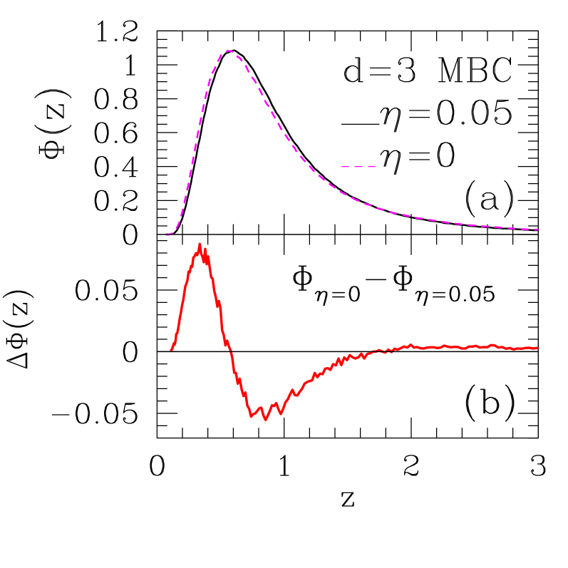
Figure 1: (a) Scaled probability distributions $\Phi(z)$ in $d=3$ with MBC, for $z$ defined in Eq. (4). Data for $L=40$, $5\times 10^{7}$ configurations. Full line: demagnetization factor $\eta=0.05$; dashed line: $\eta=0$. (b) Scaling function difference against $z$.

One sees that neglecting the demagnetizing term causes a small leftward shift of the scaling curve. As we will see in Section IV.2, the changes it causes to the fits of our distributions to the analytical $1/f^{\alpha}$ curves are of the order of systematic imprecisions characteristic of the fitting procedure. Nevertheless, it is instructive to seek the physical origins of such effect. This is done by direct inspection of the unscaled PDFs.

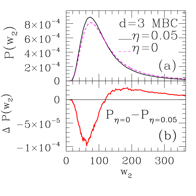
Figure 2: (a) Probability distributions $P(w_{2})$ in $d=3$ with MBC. Data for $L=40$, $5\times 10^{7}$ configurations. Full line: demagnetization factor $\eta=0.05$; dashed line: $\eta=0$. (b) Probability distribution difference against $w_{2}$. Extent of horizontal axis corresponds to the same interval of $z$–variation in Fig. 1.

In Fig. 2 it is apparent that, for $\eta=0$ the high-end tail of $P(w_{2})$ is slightly fatter than for $\eta\neq 0$, at the expense of a small amount of depletion around the most probable value of $w_{2}$. Accordingly, the average $\langle w_{2}\rangle$ is higher by $\simeq 8\%$ in the former case than in the latter (the fractional difference between averages is the same also for $d=2$ and $d=3$ PBC). Such a trend can be understood by recalling that the $\eta=0$ data have been collected just below the depinning transition, i.e., still within the regime where pinning forces are dominant. Thus the interface mostly meanders about, in order to comply with local energy minimization requests. The complement of this picture is that, for $H>H_{c}$ the interface moves with finite speed, more or less ignoring local randomness configurations, and becoming smoother the farther one is above the critical point. In short, for a given lattice size the average interface roughness decreases monotonically as the external field (driving force) is increased across its critical value.

The interpretation of the small differences between $\eta=0$ and $\eta\neq 0$ distributions is then as follows: (i) because of the way in which data for the former were collected here, they represent a system just below $H_{c}$, for which interface roughness is slightly larger than at the critical point; and (ii) the closeness of $\eta=0$ data to those for $\eta\neq 0$, and the way in which both sets of data differ, strongly suggest that behavior at the critical point of the $\eta=0$ system is the same as that of the $\eta\neq 0$ (self-regulated) case. We conclude that the self-regulating term is irrelevant, as far as critical roughness distributions are concerned.

IV.2 PBC, $d=2$ and $3$

Analytical expressions for the $1/f^{\alpha}$ distributions with PBC are either given in Ref. Antal et al., 2002 ($d=2$), or can be derived straightforwardly from Refs. Antal et al., 2002; Rosso et al., 2003b ($d=3$). In the latter case, the use of exact identities for two-dimensional lattice sums Zucker and Robertson (1975) speeds up calculations considerably. Estimates of the exponent $\zeta$ of Eq. (5), from power-law fits of simulational data with ${\cal O}(10^{6})$ events, and $400\leq L_{x}\leq 1200$ for $d=2$, $30\leq L\leq 80$ for $d=3$, give $\zeta(d=2,{\rm PBC})=1.24(1)$, $\zeta(d=3,{\rm PBC})=0.71(1)$ de Queiroz (2004).

Consideration of the scaling properties of height-height correlation functions and their Fourier transforms then suggests Rosso et al. (2003b), for the generalized Gaussian case of independent Fourier modes, that

$$\alpha=d^{\prime}+2\zeta\qquad(d^{\prime}=d-1)\ ,$$ (6)

which would imply $\alpha=3.48(2)$ ($d=2),\$3.42(2) ($d=3$).

Such predictions can be quantitatively checked by estimating the values of $\chi^{2}$ per degree of freedom ($\chi^{2}_{\rm\ d.o.f.}$) from fits of our simulation results to the analytical distributions. Since, even with $5\times 10^{7}$ samples, the simulational data eventually get frayed at the top end, given the long forward tails characteristic of all systems studied here, our fits used only data for which $\Phi(z)\geq 10^{-3}$. This turned out not to be a drastic restriction, as we were left typically with at least $100-200$ points to fit in each case.

Figure 3: $\chi^{2}$ per degree of freedom ($\chi^{2}_{\rm\ d.o.f.}$) for fits of simulation data with PBC to analytical forms of $1/f^{\alpha}$ distributions, against $\alpha$. Triangles: $d=2$, $L_{x}=400$; squares, $d=3$, $L=40$.

Assuming the uncertainty in the value of $\alpha$ that best fits our data to be given by requiring that $\chi^{2}_{\rm\ d.o.f.}$ stay within $150\%$ of its minimum, we quote from the data shown in Fig. 3: $\alpha=3.60(13)$ ($d=2$); $3.52(6)$ ($d=3$). The agreement with the above predictions is satisfactory, though slight discrepancies remain. A visual check of the goodness-of-fit for each case is given in Figs. 4 and 5.

Fitting $\eta=0$ data to the closed-form distributions produces curves whose minima of $\chi^{2}_{\rm\ d.o.f.}$ are essentially the same as in Fig. 3, and slightly shifted rightwards. Using the same criteria as above for the estimation of error bars, we have, for $\eta=0$: $\alpha=3.64(16)$ ($d=2$); $3.59(5)$ ($d=3$).

Detailed discussion, and pertinent comparisons with data from Ref. Rosso et al., 2003b, will be deferred to Section V.

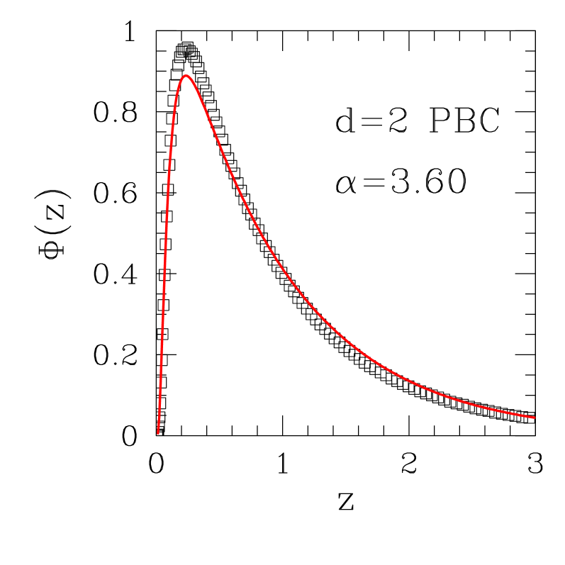
Figure 4: Scaled probability distribution $\Phi(z)$ in $d=2$ (PBC), for $z$ defined in Eq. (4), from $5\times 10^{7}$ configurations. Squares: simulation data ($L=400$). Full line is roughness distribution for $1/f^{\alpha}$ noise given in Ref. Antal et al., 2002, with $\alpha=3.60$.

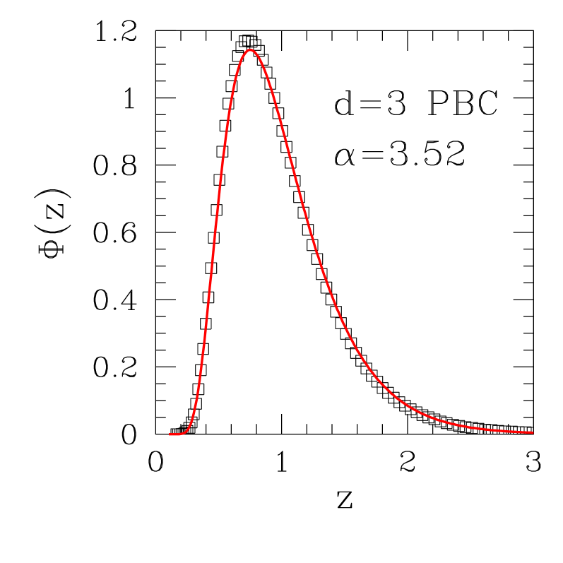
Figure 5: Scaled probability distribution $\Phi(z)$ in $d=3$ with PBC, for $z$ defined in Eq. (4), from $5\times 10^{7}$ configurations. Squares: simulation data ($L=40$). Full line is roughness distribution for $1/f^{\alpha}$ noise, with $\alpha=3.52$.

IV.3 FBC and WBC, $d=2$ and $3$

We have generated roughness data in both $d=2$ and $3$ with FBC. Our initial implementation of FBC, used also in Ref. de Queiroz, 2004, aims at a literal reproduction of the constraint that the interface must be horizontal at the edges. Thus, e.g. for $d=2$, “ghost” sites are added at $x=0$, $x=L_{x}+1$, whose heights are always adjusted to be respectively $h(0,t)=h(1,t)$, $h(L_{x}+1,t)=h(L_{x},t)$. This way, the edge sites at $x=1$ and $L_{x}$ experience no elastic pull (see the second term on the right-hand side of Eq. (1)) from their ghost neighbors outside the sample.

Similarly to the PBC cases, estimates of the exponent $\zeta$ of Eq. (5) were extracted from power-law fits of simulational data with ${\cal O}(10^{6})$ events, and $400\leq L_{x}\leq 1000$ for $d=2$, $30\leq L\leq 80$ for $d=3$. The results are $\zeta(d=2,{\rm FBC})=1.28(2)$, $\zeta(d=3,{\rm FBC})=0.89(1)$. While the former value might be construed as not inconsistent with PBC and FBC giving the same universality class for $d=2$, the same picture cannot hold for $d=3$. Though it is known Antal et al. (2001, 2002, 2004); Rosso et al. (2003b); Binder (1981) that boundary conditions do have significant influence on scaling functions of critical systems, they are not generally expected to change the values of critical exponents.

In order to discuss the roughness PDFs, we first recall the effect of FBC on $1/f^{\alpha}$ distributions. The generating function $G(s)=\int dw_{2}\,P(w_{2})\,e^{-sw_{2}}$ has the general form for PBC Antal et al. (2002); Rosso et al. (2003b)

$$G_{p}(s)=\prod_{{\bf n}\neq 0}\left(1+\frac{s}{{\bf n}^{\alpha}}\right)^{-1/2}\ ,$$ (7)

where ${\bf n}$ is a lattice vector in $d-1$ dimensions with integer coordinates. Because all ${\bf n}$ are counted, the square root disappears due to the (at least) twofold degeneracy. Requiring that the interface be horizontal at the edges implies that the Fourier representation of $h(t)$ includes only cosines. The corresponding $G_{f}(s)$ has the degeneracy of its singularities cut in half, compared to PBC.

In $d=2$, this means that the single poles found for PBC turn into square-root singularities. Evaluation of $P(w_{2})$, as the inverse Laplace transform of $G_{f}(s)$, thus necessitates a direct approach, since the residue theorem is inapplicable. This has been accomplished in Ref. Moulinet et al., 2004, from which the relevant expressions were extracted in order to attempt a minimization of $\chi^{2}_{\rm\ d.o.f}$ against $\alpha$, similar to that of Section IV.2. With $\zeta(d=2,{\rm FBC})$ as above, one would expect a good fit for $\alpha\simeq 3.5-3.6$. Instead, $\chi^{2}_{\rm\ d.o.f}$ has a minimum value $\simeq 4\times 10^{-3}$ at $\alpha=2.96$, and increases monotonically to reach $\simeq 4\times 10^{-2}$ at $\alpha=3.5$. This is clearly at variance with correspondings results for the PBC case.

We then decided to generate data using window boundary conditions (WBC) Antal et al. (2002); Moulinet et al. (2004), which are generally accepted as an alternative way to simulate free edges. Accordingly, in $d=2$ we imposed global PBC on a system of overall length $L_{x}$, and measured the local roughness within each of $n_{w}$ adjacent windows of length $L_{x}/n_{w}$. With $n_{w}\gg 1$, it is plausible to assume that the resulting PDFs are independent of the boundary conditions established at $x=0$, $L_{x}$. In order to guarantee statistical independence, one should in principle use widely separated windows. However, the use of nonoverlapping, but neighboring, windows instead appears to introduce no measurable errors on the resulting PDFs Antal et al. (2002). We fixed $n_{w}=10$, and initially measured $\zeta$ via Eq. (5), from a sequence of simulations with ${\cal O}(10^{6})$ events (i.e. individual avalanches, thus the total number of roughness samples is larger by a factor of $n_{w}$), and $400\leq L_{x}\leq 1200$, which gave $\zeta(d=2,{\rm WBC})=1.21(2)$. Though this differs by $3.5$ standard deviations from the value coming from FBC, it is just consistent, at the margin, with $\zeta(d=2,{\rm PBC})=1.24(1)$ found above.

Direct examination of scaled PDFs results in the following observations. First, in Figure 6 one can see that the PDFs in $d=2$ for FBC and WBC are unmistakably distinct. Furthermore, fits of FBC data to the analytical expressions derived in Ref. Moulinet et al., 2004 have been found to be generally of low quality. As mentioned above, the best fit of FBC data is for the $\alpha=2.96$ curve, shown in the Figure as a dashed line, and corresponds to $\chi^{2}_{\rm\ d.o.f.}\simeq 4\times 10^{-3}$. Though this average deviation is of the same order as that for the best case with PBC (recall Fig. 3), comparison to Fig. 4 shows that, while for PBC discrepancies are concentrated close to the narrow peak (thus they can be at least partially ascribed to binning effects), here one has a rather widespread disagreement in shape.

On the other hand, WBC data can be much more closely fitted by the analytical expressions, as shown both in the inset of Fig. 6, where $\chi^{2}_{\rm\ d.o.f.}$ exhibits a minimum value $\simeq 7\times 10^{-4}$ at $\alpha=3.85$, and directly in the main Figure, by the superposition of the $\alpha=3.85$ curve onto the corresponding numerical data.

In summary, an analytical form derived from assuming an interface whose Fourier representation has only cosines (i.e. is horizontal at the edges) has provided a very good fit to numerical data generated by imposing WBC. Though this appears contradictory, the same procedure has been successfully accomplished in Ref. Moulinet et al., 2004, with regard to both experimental and simulational data.

Still, an important question remains, since the optimum $\alpha=3.85(5)$ (error bars estimated as in Section IV.2) implies $\zeta=1.43(3)$ via Eq. (6). This is significantly distinct from all three estimates thus far obtained for $d=2$, which average to 1.25(5). We shall defer the discussion of this point to Section V.

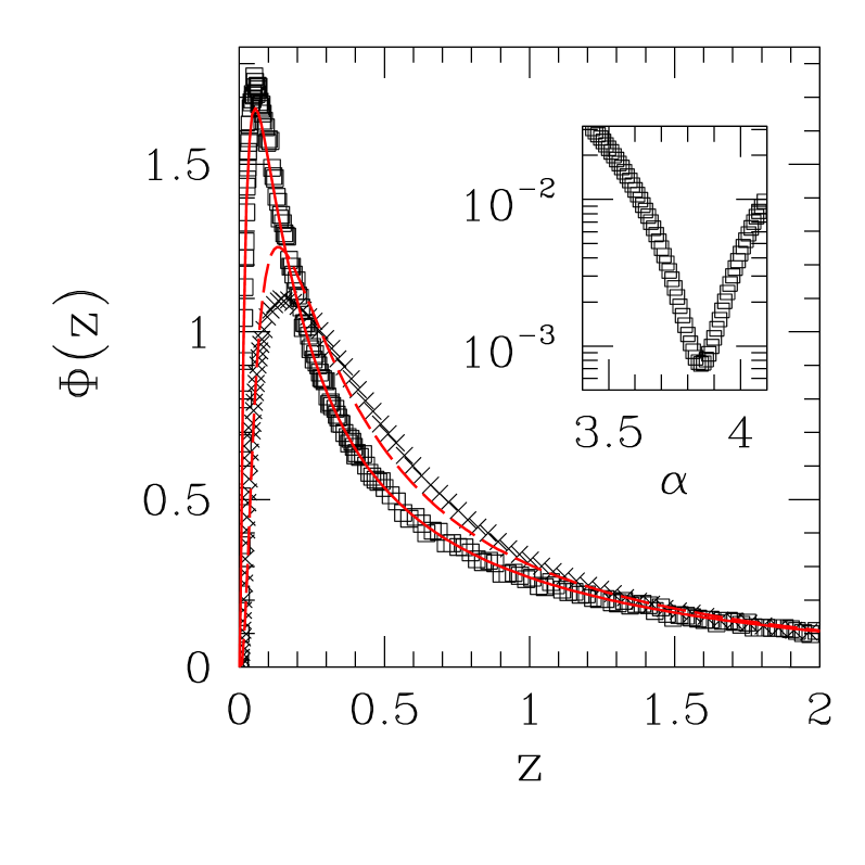
Figure 6: Scaled probability distribution $\Phi(z)$ in $d=2$, for $z$ defined in Eq. (4). Points are simulation data. Crosses: $L=400$, FBC, $5\times 10^{7}$ configurations. Squares: $L=400$, WBC, $10^{7}$ avalanches, $n_{w}=10$ windows. Full line is roughness distribution for $1/f^{\alpha}$ noise (see Ref. Moulinet et al., 2004), with $\alpha=3.85$. Dashed line : roughness distribution for $\alpha=2.96$ (see text). Inset: $\chi^{2}_{\rm\ d.o.f.}$ against $\alpha$, for fits of WBC simulation data against $1/f^{\alpha}$ distributions, showing a minimum at $\alpha=3.85$.

Turning now to $d=3$, all poles of $G_{p}(s)$ have even degeneracy. A straightforward adaptation for FBC is as follows. Recalling that the lattice sums $\sum_{{\bf n}}|{\bf{n}}|^{-\alpha}$ which crop up in the calculation of $\langle w_{2}\rangle$ Antal et al. (2001, 2002); Rácz and Plischke (1994) must be halved, this implies a rescaling of the variable $s$, so formally one can write Antal et al. (2002):

$$G_{f}(s)=\sqrt{G_{p}(2s)}\ .$$ (8)

Fitting our $d=3$ FBC data to analytical distribution functions, obtained with help of Eq. (8), turns out to give similar results to the $d=2$ case. The above-quoted value $\zeta=0.89(1)$, from the finite-size scaling of $\langle w_{2}\rangle$, together with Eq. (6), would suggest $\alpha=3.78(2)$. However, $\chi^{2}_{\rm\ d.o.f.}$ against $\alpha$ has a single minimum ($\simeq 10^{-3}$) at $\alpha=3.18(8)$ (error bars estimated as in Section IV.2) and increases monotonicaly, reaching $\simeq 2\times 10^{-2}$ at $\alpha=3.78$.

We again resorted to WBC. Imposing PBC at the edges of a system with $L\times L$ cross-section, we measured local roughness within each of $n_{w}$ non-overlapping, adjacent, square windows of linear dimension $L/\sqrt{n_{w}}$ (or the largest integer contained in it). We took $n_{w}=16$, and initially measured $\zeta$ from a sequence of simulations with ${\cal O}(10^{6})$ events, and $30\leq L\leq 80$, which gave $\zeta(d=3,{\rm WBC})=0.75(2)$. The discrepancy between this and the value $0.89(1)$ coming from FBC is rather more severe than the corresponding case for $d=2$. On the other hand, the present estimate is close to the values of $\zeta(d=3,{\rm PBC})$ found above, namely $0.71(1)$ from Eq. 5, and $0.76(3)$ from optimization of fits against $1/f^{\alpha}$ distributions plus Eq. 6.

Again, we investigated the roughness PDFs generated with WBC. Similarly to the $d=2$ case, they differ markedly from the ones obtained with FBC, as shown in Fig. 7 . This time, fits against the analytical expressions given through Eq. (8) exhibit a deep, well-defined minimum of $\chi^{2}_{\rm\ d.o.f.}$ at $\alpha=3.76(5)$ (see inset in the Figure), in very good agreement with $\alpha=3.78(2)$ predicted from finite-size scaling of $\langle w_{2}\rangle$ data for FBC, together with Eq. (6). However, for reasons to be explained at length in Section V, we believe this coincidence to be accidental.

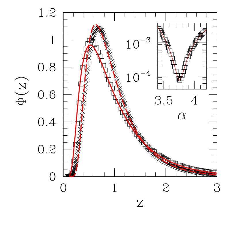
Figure 7: Scaled probability distribution $\Phi(z)$ in $d=3$, for $z$ defined in Eq. (4). Points are simulation data. Crosses: $L=40$, FBC, $5\times 10^{7}$ configurations. Squares: $L=40$, WBC, $3\times 10^{7}$ avalanches, $n_{w}=16$ windows. Lines are roughness distributions for $1/f^{\alpha}$ noise (see Eq. (8)), with $\alpha=3.76$ (full) and $3.18$ (dashed). Inset: $\chi^{2}_{\rm\ d.o.f.}$ against $\alpha$, for fits of WBC simulation data against $1/f^{\alpha}$ distributions, showing a minimum at $\alpha=3.76$.

IV.4 MBC, $d=3$

We started by studying systems with a square cross-section, imposing PBC along $x$ and FBC, as defined at the beginning of Section IV.3, along $y$.

Estimates of the exponent $\zeta$ of Eq. (5) were again extracted from power-law fits of simulational data with ${\cal O}(10^{6})$ events, and $30\leq L\leq 80$ for $d=3$ MBC, with the result $\zeta(d=3,{\rm MBC})=0.87(1)$ de Queiroz (2004).

The Fourier representation of $h(t)$ with MBC can be put in the form:

$$h(x,y)=\sum_{m,n}c_{mn}\,e^{2\pi i\left(mx+\frac{n}{2}y\right)/L}\ ,$$ (9)

where $m,n=0,\pm 1,\pm 2,\dots$, $(m,n)\neq(0,0)$, and $c_{-m,n}=c^{\ast}_{m,n}$; $c_{m,-n}=c_{m,n}$. Thus a global rescaling such as that of Eq. (8) is not possible. On the other hand, starting from Eq. (9), an analysis similar to that of Refs. Antal et al., 2002; Rácz and Plischke, 1994 suggests a generating function:

$$G_{m}(s)=\prod_{m,n}\left(1+\frac{s}{(4m^{2}+n^{2})^{\alpha/2}}\right)^{-1/2}\ ,$$ (10)

again with $(m,n)\neq(0,0)$. The double sum $\sum_{m,n}(4m^{2}+n^{2})^{-\alpha/2}$, which appears in the subsequent expression for $\langle w_{2}\rangle$, corresponds to ${\cal Q}(1,0,4)$ of Ref. Zucker and Robertson, 1975 and can be easily evaluated.

We performed fits of simulational data to the closed-form PDFs calculated as above. While Eq. (6), with $\zeta=0.87(1)$, gives $\alpha=3.74(2)$, $\chi^{2}_{\rm\ d.o.f}$ has a minimum $\simeq 2\times 10^{-3}$ at $\alpha=3.36(10)$. The overall quality of fits is slightly worse than for $d=3$ FBC (refer to Fig. 7).

In order to investigate WBC, we took rectangular systems with dimensions $L_{x}$ and $L_{y}=4\,L_{x}$ with full PBC (we denote this setup as mixed window boundary conditions (MWBC)) and calculated local roughness distributions within $n_{w}=4$ square windows of $L_{x}\times L_{x}$ sites each, side by side along the $y$ axis. Scaling of the first moment of the distribution, Eq. (5), with $30\leq L_{x}\leq 80$, gave $\zeta=0.74(1)$.

Again, the roughness PDF thus obtained was markedly distinct from that with MBC. In addition, fits to the analytical expressions derived from Eq. (10) were considerably worse than those of MBC data, with a minimum $\chi^{2}_{\rm\ d.o.f}\simeq 1\times 10^{-2}$ at $\alpha=4.1$.

The results are displayed in Fig. 8, where it can be seen that even the best-fitting analytical PDF fails to provide a good match to the MWBC data (except for the initial, rather steep, ascent close to $z=0$).

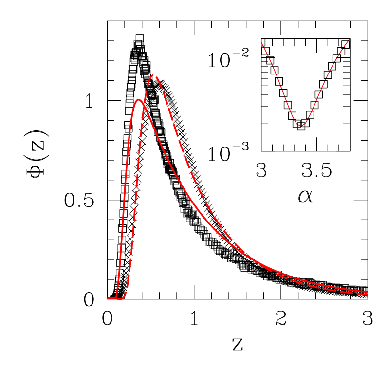
Figure 8: Scaled probability distribution $\Phi(z)$ in $d=3$, for $z$ defined in Eq. (4). Crosses: simulation data ($L=40$, MBC, $5\times 10^{7}$ configurations). Squares: simulation data ($L_{x}=40$, $L_{x}=160$, MWBC (see text), $3\times 10^{6}$ avalanches, $n_{w}=4$ windows). Lines are roughness distributions for $1/f^{\alpha}$ noise (see Eq. (10)), with $\alpha=4.1$ (full) and $3.36$ (dashed). Inset: $\chi^{2}_{\rm\ d.o.f.}$ against $\alpha$, for fits of MBC simulation data against $1/f^{\alpha}$ distributions, showing a minimum at $\alpha=3.36$.

V Discussion and Conclusions

We begin our discussion by recalling from Ref. de Queiroz, 2004 and Sec. IV.2 that, for the model considered here with PBC, the finite-size scaling of the first moment of the distribution gives $\zeta(d=2,{\rm PBC})=1.24(1)$, $\zeta(d=3,{\rm PBC})=0.71(1)$. Both compare well with the usually accepted values for the quenched Edwards-Wilkinson (EW) universality class Leschhorn (1993); Makse and Amaral (1995); Makse et al. (1998); Rosso et al. (2003a), respectively $\zeta\simeq 1.25$ ($d=2$) and $\zeta\simeq 0.75$ ($d=3$). Furthermore, consideration of the full distributions points the same way: our simulational data displayed in Figs. 4 and 5 match very well those in Figure 2 of Ref. Rosso et al., 2003b which concern the EW model. The agreement with EW behavior is consistent with our results of Sec. IV.1 regarding the independence of scaled roughness distributions on the demagnetizing term. Indeed, the quenched EW equation can be written as Rosso et al. (2003a)

$$\frac{\partial h({\bf x},t)}{\partial t}=u({\bf x},h)+a\,\nabla^{2}h({\bf x})+f\ ,$$ (11)

where $u$ represents quenched disorder and $f$ is the external driving force. This has a one-to-one correspondence with Eq. (1), except that in that Equation we allowed for the self-regulating, demagnetizing, term. Having shown that such mechanism is irrelevant as far as scaled roughness distributions are concerned, it becomes tenable to assume that, overall, our model belongs to the EW universality class.

Still for PBC, the connection between the exponents $\alpha$ and $\zeta$, predicted Rosso et al. (2003b) in Eq. (6), is verified within reasonable error bars.

Turning to different sets of boundary conditions, we first point out that small differences in implementation of FBC (namely, “literal” FBC, i.e. horizontal interface at the edges, versus WBC) significantly alter the roughness PDFs. The question then arises of which, if any, of these implementations is the “right” one.

We investigate this by referring to results derived through a “proven” method, i.e. finite-size scaling of the first moment of the distribution. Examination of the corresponding column of Table 1 strongly suggests that, in both $d=2$ and $3$, WBC (including WMBC) preserves universality with PBC, while FBC does not (though in $d=2$ FBC does not perform very badly). Accepting such preservation as a basic tenet, we conclude that FBC as implemented induces strong distortions in the scaling behavior of interface roughness. In this context, the good agreement in $d=3$ between the optimum $\alpha$ for fits of WBC data to the analytical forms, and that coming from finite-size scaling of FBC data via Eqs. (5) and (6), must be regarded as fortuitous.

Thus, we discard FBC, as well as MBC, for the remaining of the present discussion. One must note, however, that use of MBC (i.e. partial FBC) provides a sensible representation of the physical setup found in thin films, as well as reproducing well-known results (concerning scaling behavior of avalanche sizes) at both ends of the crossover between $d=2$ and $3$ de Queiroz (2004).

Table 1: Estimates of roughness exponent $\zeta$ for different dimensionalities and boundary conditions (BC). $\zeta^{\rm FSS}$: finite-size scaling of first moment of distribution, Eq. (5). $\zeta_{\rm fit}$: from best-fitting $1/f^{\alpha}$ distribution and Eq. (6). $\chi^{2}_{\rm\ d.o.f.}$ (min): value of $\chi^{2}_{\rm\ d.o.f.}$ for $\zeta=\zeta_{\rm fit}$.

	$\zeta^{\rm FSS}$	$\zeta_{\rm fit}$	$\chi^{2}_{\rm\ d.o.f.}$ (min)
$d=2$ PBC	$1.24(1)$	$1.30(8)$	$6\times 10^{-4}$
$d=2$ FBC	$1.28(2)$	$0.98(7)$	$4\times 10^{-3}$
$d=2$ WBC	$1.21(2)$	$1.42(3)$	$7\times 10^{-4}$
$d=3$ PBC	$0.71(1)$	$0.76(3)$	$3\times 10^{-4}$
$d=3$ FBC	$0.89(1)$	$0.59(4)$	$1\times 10^{-3}$
$d=3$ WBC	$0.75(2)$	$0.88(1)$	$8\times 10^{-5}$
$d=3$ MBC	$0.87(1)$	$0.68(5)$	$2\times 10^{-3}$
$d=3$ MWBC	$0.74(1)$	$1.05(10)$	$1\times 10^{-2}$

Returning to roughness scaling, we see in Table 1 that the fair agreement between $\zeta^{\rm FSS}$ and $\zeta_{\rm fit}$, found for PBC in $d=2$ and $3$, is absent in the remaining cases under consideration, i.e. $d=2$ WBC, $d=3$ WBC, $d=3$ MWBC. One might ask whether finite-size effects (though widely believed to vanish already for small lattices Antal et al. (2001, 2002); Rosso et al. (2003b); Foltin et al. (1994)) still have a nonnegligible quantitative effect on the scaled roughness PDFs found here, so as to distort our fits to the analytical distributions. We present data to show that this is not the case.

In Figure 9 we compare $L=40$ and $L=80$ PDFs, for $d=3$ WBC. Contrary to the systematic trend exhibited in Fig. 1 (for comparison between $\eta=0$ and $\neq 0$ distributions), here the difference $\Delta\Phi(z)$ is rather small and essentially random, arising because of fluctuations in statistics, coupled with binning effects. An apparently systematic effect shows up only for the narrow range close to $z=0$ where both PDFs have a steep slope. That, however, involves only of order $5-10$ points, with a consequently reduced effect on the overall statistics. The corresponding curves $\chi^{2}_{\rm\ d.o.f.}$ against $\alpha$ are nearly indistinguishable; with $L=80$ data, the minimum of $\chi^{2}_{\rm\ d.o.f.}$ is $9\times 10^{-5}$ at $\alpha=3.76(4)$, virtually identical to the $L=40$ result shown in Fig 7 (see also Table 1). For $d=2$ WBC and $d=3$ MWBC, the overall picture is the same. Therefore, finite-size effects on the numerically-obtained PDFs are not a likely source for the disagreements found.

Figure 9: (a) Scaled probability distributions $\Phi(z)$ in $d=3$ with WBC, for $z$ defined in Eq. (4). Squares: $L=40$. Full line: $L=80$. In both cases, $10^{6}$ avalanches, $n_{w}=16$ windows. (b) Scaling function difference against $z$.

We note also that, when considering $1/f^{\alpha}$ distributions, there is no apparent reason why Eq. (6) should not hold for boundary conditions other than PBC, as that Equation was derived for generalized Gaussian distributions Rosso et al. (2003b) with the only assumption that the large-scale behavior is determined by a single observable.

We are thus left with a single point to analyze, namely the overall adequacy of $1/f^{\alpha}$ distributions to describe the problem at hand. The following comments are in order:

(1) already for PBC, the study of generalized depinning problems shows that small but systematic discrepancies remain between numerical data and $1/f^{\alpha}$ PDFs, whose origins can be traced to higher cumulants of the correlation functions Rosso et al. (2003b). Thus, in this sense the $1/f^{\alpha}$ distributions are not expected to be a perfect fit, even for PBC.

(2) In Ref. Moulinet et al., 2004 the equation of motion for $h(x)$ contains a long-range elastic term, $\int dx_{1}\,\left(h(x)-h(x_{1})\right)/(x-x_{1})^{2}$, instead of the local term, $\nabla^{2}h({\bf x})$, present here. While in that case an $1/f^{\alpha}$ distribution gives good fits to the numerically-generated roughness PDF with WBC, this does not necessarily imply that a similar quality of fit can be found for the present EW problem with WBC. In this connection, one might ask how far the independent Fourier mode assumption, basic in the derivation of $1/f^{\alpha}$ PDFs, is affected by such details. One sees that the long-range term contributes qualitatively in the same direction as PBC, i.e. by imposing additional constraints on interface roughness (when compared, respectively, to short-range interactions and WBC).

A plausible scenario then emerges, in which the amplitude of corrections to the representation of an interface roughness PDF by an $1/f^{\alpha}$ distribution would depend on how much that interface is constrained, either by boundary conditions or by elastic terms in the equation of motion. Lessening of such constraints would imply an increase in the correction amplitudes. However, at present we do not see a way to quantify and test these remarks.

Clearly, more work is needed in order to clarify the connection between $1/f^{\alpha}$ distributions and generalized depinning transitions.