Variational theory for a single polyelectrolyte chain revisited

Abstract

We reconsider the electrostatic contribution to the persistence length, $\ell_{e}$, of a single, infinitely long charged polymer in the presence of screening. A Gaussian variational method is employed, taking $\ell_{e}$ as the only variational parameter. For weakly charged and flexible chains, crumpling occurs at small length scales because conformational fluctuations overcome electrostatic repulsion. The electrostatic persistence length depends on the square of the screening length, $\ell_{e}\sim\kappa^{-2}$, as first argued by Khokhlov and Khachaturian by applying the Odijk-Skolnick-Fixman (OSF) theory to a string of crumpled blobs. We compare our approach to previous theoretical works (including variational formulations) and show that the result $\ell_{e}\sim\kappa^{-1}$ found by several authors comes from the improper use of a cutoff at small length scales. For highly charged and stiff chains, crumpling does not occur ; here we recover the OSF result and validate the perturbative calculation for slightly bent rods.

1 Introduction

Charged polymer chains, also called polyelectrolytes, have many industrial applications (flocculants, viscosifiers, adsorbants, etc.) related to their large solubility in water, which is present even for a highly hydrophobic backbone. They are also important in biology since many biopolymers (such as nucleic acids) are charged.

In this paper we reconsider the controversial issue of the dependence of the persistence length of polyelectrolytes on electrostatic interactions and, consequently, on the salt concentration in water, which has been of central interest during the past few years Forster ; BarratRev ; NetzRev . This is an important question with a large number of experimental implications, since for instance, many properties of biological and synthetic polymers depend on their stiffness and thus on the salt concentration in the solution. It is therefore an important control parameter. Most of the theoretical attempts have treated electrostatic interactions on the linear Debye-Hückel level, leaving aside the very important effects connected with counterion condensation (which can be obtained on the mean-field level by properly taking non-linear effects into account) and with strong electrostatic correlations, important when multivalent ions are present kardar ; shklovskii ; ariel . Here we use the same simplifying assumptions. Our purpose is therefore not to describe experiments or simulations (with explicit counterions) better than previous calculations, but to detect and eliminate inherent methodological shortcomings and inconsistencies in some of the previous calculations, which led to controversial results. Our results should therefore not be compared with experiments, but rather with one of the many simulations of polymer chains where Debye-Hückel repulsions are used Micka ; Stevens ; Everaers ; Nguyen ; Ullner . Especially the disagreement between a number of previous variational calculations is highly irritating Schmidt ; Barrat ; Bratko ; Li ; Thirumalai1 ; Netz ; Thirumalai2 : variational calculations are typically known to be very robust, reliable and therefore useful in a wide range of physics applications. The immediate question therefore should be : is there any ingredient in fluctuating charged polymers that forbids the use of a variational theory ? The answer we give in this paper is clearly negative. Variational methods do work for charged polymers as they do for superconductivity, strongly correlated electron systems, protein folding, random media, etc. This makes our methods in principle also applicable to more complicated problems such as polymer solutions and the coupling between counterion condensation and chain stiffening (which we will tackle in the future).

Our calculational strategy consists in constructing the simplest variational Gaussian correlation function which i) reflects the stiffening of the chain at small length scales, but at the same time, ii) leads to a converging variational free energy and therefore makes introduction of a small-scale cutoff (as used in previous calculations) unnecessary. Quite surprisingly, the simple worm-like chain correlation function does not satisfy criterion ii) and therefore has to be discarded. The simplest workable correlation function, related to the tangent-tangent correlation function, shows a two-scale behaviour, in agreement with previous perturbative calculations BarratRev . It explains why the electrostatic persistence length is difficult to extract in experiments or simulations. As our main result, we obtain that, in the flexible polymer case, where the chain crumples at small length scales and forms a persistent chain of Gaussian blobs (Gaussian-persistent regime), the electrostatic persistence length depends on the square of the screening length, $\ell_{e}\sim\kappa^{-2}$. We thus confirm the scaling theory by Khokhlov and Khachaturian KK who applied the Odijk-Skolnick-Fixman (OSF) Odijk ; SF theory to a string of crumpled blobs. This is in accordance with previous theoretical studies Netz ; Thirumalai2 and very recent simulations Everaers ; Nguyen . The uncontrolled usage of a cutoff at small length scales seems to be the origin of the very different results for the persistence length found in previous papers. In the next section, we summarize previous calculations for the persistence length of charged polymers. In Section 3, we present the general scheme of our calculations both for flexible and stiff chains. In Section 4, we study the case of flexible chains, using a variational Hamiltonian which exhibits a crossover from crumpled statistics at small scales to rod-like behaviour at intermediate scales. We show both numerically and analytically in the asymptotic limit of low ionic strength that $\ell_{e}\sim\kappa^{-2}$. In Section 5, we return to the case of stiff polymers, the persistent regime, and show why the worm-like-chain model cannot be used per-se for a variational approach. This is related to the behaviour at small scales. We use a slightly more complicated variational kernel which regularizes the small-scale behaviour and recover variationally the classical Odijk-Skolnick-Fixman result. Section 6 is devoted to the discussion of our results and the comparison with previous theoretical calculations. Finally in Section 7, we give our concluding remarks.

2 Previous Results

The first studies of the influence of electrostatic interactions on polyelectrolyte stiffness have been done by Odijk Odijk and Skolnick and Fixman SF . By performing a perturbation calculation on a slightly bent rigid charged rod using the Debye-Hückel approximation, they found that the total persistence length is

$$\ell_{p}=\ell_{0}+\ell_{e}$$ (1)

where $\ell_{0}$ is the bare persistence length and $\ell_{e}$ the electrostatic contribution:

$$\ell_{e}=\ell_{\mathrm{OSF}}=\frac{\ell_{B}}{4A^{2}\kappa^{2}}$$ (2)

The length $\ell_{B}=e^{2}/(4\pi\epsilon k_{B}T)$ is the Bjerrum length (the distance between two elementary charges interacting with the thermal energy $k_{B}T$), $A$ the distance between charges along the chain and $\kappa=[4\pi\ell_{B}(c_{+}+c_{-})]^{1/2}$ the Debye-Hückel parameter, related to micro-ion concentrations, $c_{\pm}$. This result is valid for polymer conformations which do not deviate too much from the rod-like reference state, i.e. for stiff polymers with a large bare persistence length, $\ell_{B}\ell_{0}/A^{2}\gg 1$, and sufficient screening. In a systematic derivation, Barrat and Joanny found that the electrostatic stiffening is actually scale-dependent and $\ell_{e}$ as given by Eq. (2) is only realized at large scales Barrat .

The case of flexible polymers, however, remained somewhat unclear and a host of controversial results can be found in the literature. On one hand, Khokhlov and Khachaturian KK (KK) assumed that the OSF theory can be applied to a chain of polyelectrolyte blobs in the case of weakly charged flexible polyelectrolytes. At short length scales, the electrostatic repulsion is weaker than the chain entropy. The electrostatic blob size, $\xi\simeq\ell_{0}n^{1/2}$ where $n$ is the number of monomers (each of size $\ell_{0}$) in the blob, is defined by the requirement that the electrostatic energy of the Gaussian polymer coil is equal to the thermal energy, that is $(n\ell_{0}/A)^{2}\ell_{B}/\xi\simeq 1$. The blob size follows as

$$\xi\simeq\ell_{0}\left(\frac{\ell_{B}\ell_{0}}{A^{2}}\right)^{-1/3}$$ (3)

and the number of monomer in the blob is

$$n\simeq\left(\frac{\ell_{B}\ell_{0}}{A^{2}}\right)^{-2/3}$$ (4)

At a scaling level, the effective distance between charges along the direction of the string of blobs is then renormalized by the linear density of monomers, $A^{\prime-1}\simeq\frac{\ell_{0}n}{\xi}A^{-1}$. By replacing $A$ by $A^{\prime}$ in Eq. (2), KK found

$$\ell_{e}=\ell_{\mathrm{KK}}\simeq\left(\frac{\ell_{B}\ell_{0}}{A^{2}}\right)^{1/3}\frac{1}{\ell_{0}\kappa^{2}}$$ (5)

which exhibits the same dependence in $\kappa^{-2}$ as the OSF result. This has been confirmed by Li and Witten who studied the effect of chain fluctuations in the presence of screening and showed that they do not affect the value of $\ell_{e}$ found by KK Li .

On the other hand, using a variational approach by modelling the flexible polyelectrolyte as a chain under tension, Barrat and Joanny Barrat found a different $\kappa$ dependence:

$$\ell_{e}=\ell_{\mathrm{BJ}}\simeq\frac{1}{\kappa}$$ (6)

This result is consistent with a scaling argument proposed by de Gennes et al. PGG for solutions and has also been found by Pfeuty Pfeuty using the Renormalization Group theory. More recent renormalization calculations have been done by Liverpool and Stapper Liverpool2 and point to a similar (even sublinear) dependence of the persistence length on $\kappa$. A number of different approaches led to the same behaviour : i) an approach based on minimization of an approximated free energy Schmidt , ii) a $1/d$ expansion (where $d$ is the space dimension) Rudi , and iii) variational approaches Thirumalai1 using the “uniform expansion” method first derived by Edwards and Singh Singh ; DE .

It is important to mention that the result Eq. (6) poses problems at the crossover charge $\ell_{B}\ell_{0}\simeq A^{2}$, between the Gaussian-persistent and the persistent regime. The $\kappa$ dependence for $\ell_{e}$ is then not continuous and a crossover formula should be found in theories. Among theoretical works which predict Eq. (6), there is no satisfying answer to this question.

Recently, Netz and Orland Netz used the most general Gaussian kernel for the variational Hamiltonian Jonsson1 and recovered the well-known three distinct scaling regimes, defined according to the value of the screening parameter $\kappa\ell_{0}$ and the charge parameter $\ell_{B}\ell_{0}/A^{2}$. For weakly charged polymers and at large screening, one is in the Gaussian regime where the notion of electrostatic persistence length is meaningless. At small screening, and according to the charge and the stiffness of the chain (for $\ell_{B}\ell_{0}/A^{2}>1$), one reaches the persistent regime where $\ell_{e}$ is given by the OSF result, equation (2). The Gaussian-persistent regime is reached when the electrostatic repulsion between monomers is weaker (for $\ell_{B}\ell_{0}/A^{2}<1$) and the chain is crumpled at small length scales. It is shown that in this last regime, the asymptotic electrostatic persistence length (when $\kappa\ell_{0}\rightarrow 0$) is given by the KK result, equation (5).

Although the work by Netz and Orland is in accord with the growing consensus that the KK result is asymptotically correct, it uses quite complicated mathematics and cannot be easily extended to other systems, such as polyelectrolyte solutions. Moreover, the persistence length is found quite indirectly by matching the small-distance behaviour with the asymptotic swelling range due to excluded volume interactions. Hence, the intermediate distance range where the chain statistics is truly Gaussian at scales larger than the persistence length is not considered. However, such an intermediate range always exists provided that $\ell_{p}\gg\kappa^{-1}$ which is typically the case both in the persistent and the Gaussian-persistent regimes NetzRev . The persistence length should thus be determined by the crossover between the persistent range and the intermediate Gaussian range. Finally, in order to compare to experiments and simulations, it would be interesting to find the $\kappa$-dependence also near the crossover, $\kappa\xi\simeq 1$, where screening becomes important, and not only asymptotically. These are the reasons that motivated this study where the variations of $\ell_{e}(\kappa)$ are determined self-consistently by choosing $\ell_{e}$ as the variational parameter.

In a number of papers a similar single-parameter variational theory was used, but the variational persistence length reflected the swelling behaviour of the chain for large scales Muthu2 ; Ghosh ; Yethiraj ; Donley1 ; Donley2 ; Winkler . This is borne out by the fact that the persistence length depends on the chain length with a characteristic power law $\ell_{e}\sim N^{\gamma}$ which in the infinite chain limit $N\rightarrow\infty$ gives the correct swelling behaviour for the radius of gyration. In these calculations, the persistence length does not reflect the mechanical properties of the chain at small length scales, because one would expect the persistence length to saturate to a finite value as $N\rightarrow\infty$. In our paper, in contrast, we fix the large-scale behaviour as being Gaussian (thus corresponding to the actual intermediate regime for real chains) and the variational parameter reflects the transition from the rod-like to the Gaussian behaviour. The reason for this choice is that taking into account both the stiffening (at small length scales) and the swelling (at large length scales) requires two distinct variational parameters, a formidable task which can be done only asymptotically and within uncontrolled approximations Netz .

3 Model

In the following, we consider a Gaussian charged polymer in a solution of monovalent salt (concentrations $c_{+}$ for cations and $c_{-}$ for anions). The polymer chain of polymerization index $N$ and a chain length $L=N\ell_{0}$ is supposed uniformly charged with quenched charges $+e$. The distance between charges along the chain is given by $A$. We remain at the linear level for electrostatic interactions, assuming a Debye-Hückel screened interaction between charges due to the presence of monovalent counterions and salt. As explained in the Introduction, we therefore neglect non-linear effects connected to counterion condensation at low salt concentrations (we plan to incorporate such effects in the future by using a modified variational action; in the present paper we mostly try to resolve inconsistencies in previous treatment of this linear model). We use a continuous description of the polymer, parameterized by the curvilinear index $s$ and where $\mathbf{r}(s)$ is the position of the monomer labelled by $s$. The Hamiltonian of the system is LNN ; Muthu2 ; Winkler

$$\beta\mathcal{H}[\mathbf{r}] = \beta\mathcal{H}_{\mathrm{el}}[\mathbf{r}]+\beta\mathcal{H}_{\mathrm{stiff}}[\mathbf{r}]+\beta\mathcal{H}_{\mathrm{int}}[\mathbf{r}]$$ (7)

$$= \frac{1}{2}\int_{0}^{L}\mathrm{d}s\left[\frac{3}{2\ell_{0}}\mathbf{\dot{r}}^{2}(s)+\frac{3\ell_{0}}{2}\mathbf{\ddot{r}}^{2}(s)\right]$$

$$+ \frac{\ell_{B}}{2A^{2}}\int_{0}^{L}\mathrm{d}s\int_{0}^{L}\mathrm{d}s^{\prime}\frac{\exp(-\kappa|\mathbf{r}(s)-\mathbf{r}(s^{\prime})|)}{|\mathbf{r}(s)-\mathbf{r}(s^{\prime})|}$$

where $\beta=(k_{B}T)^{-1}$. The first term is the standard elasticity of entropic origin, the second one the bending stiffness of the chain, and the last term the electrostatic interaction. The partition function is

$$\mathcal{Z}=\int\mathcal{D}\mathbf{r}\exp\{-\beta\mathcal{H}[\mathbf{r}]\}$$ (8)

and is intractable due to the electrostatic term.

To make progress, we choose a variational Gaussian Hamiltonian which most generally reads

$$\beta\mathcal{H}_{0}[\mathbf{r}]=\frac{1}{2}\int_{0}^{L}\mathrm{d}s\int_{0}^{L}\mathrm{d}s^{\prime}\mathbf{r}(s)g^{-1}(s-s^{\prime})\mathbf{r}(s^{\prime})$$ (9)

where $g^{-1}$ is the Gaussian kernel. Gaussian statistics implies that $g$ is the monomer-monomer correlation function:

$$\langle\mathbf{r}(s)\mathbf{r}(s^{\prime})\rangle_{0}=3g(s-s^{\prime})$$ (10)

where $\langle...\rangle_{0}$ denotes the expectation value computed with the variational Hamiltonian (9). It is related to the squared monomer separation as

$$\langle[\mathbf{r}(s)-\mathbf{r}(s^{\prime})]^{2}\rangle_{0}=G(s-s^{\prime})=6g(0)-6g(s-s^{\prime})$$ (11)

The tangent-tangent correlation function is simply

$$\langle\mathbf{\dot{r}}(s)\mathbf{\dot{r}}(s^{\prime})\rangle_{0}=3\frac{\partial^{2}}{\partial s\partial s^{\prime}}g(s-s^{\prime})=\frac{1}{2}G^{\prime\prime}(s-s^{\prime})$$ (12)

The variational free energy reads in the Gibbs-Bogoliubov form

$$F_{\mathrm{var}}=F_{0}+\langle\mathcal{H}-\mathcal{H}_{0}\rangle_{0}$$ (13)

where $\beta F_{0}=-\ln\mathcal{Z}_{0}$ is the free energy associated with the variational Hamiltonian defined in equation (9). The Gibbs inequality ensures that $F_{\mathrm{var}}\geq F_{\mathrm{exact}}$ when $F_{\mathrm{var}}$ is minimized with respect to the variational parameters. As we are interested in the persistence length, we will choose the electrostatic contribution $\ell_{e}$ (to be defined below) as the only variational parameter. The value of the persistence length will thus be determined by minimizing equation (13) with respect to $\ell_{e}$. It must be emphasized, however, that we will restrict our choice of variational Hamiltonians to the subclass of non-swollen (ideal) correlations at large scales, and by doing so, we do not obtain the true minimum of the variational free energy.

Before starting explicit calculations, it is useful to consider the Hamiltonian (7) and to rescale all lengths by the bare persistence length according to $r=\ell_{0}\tilde{r}$ and $s=\ell_{0}\tilde{s}$. We obtain

$$\beta\mathcal{H}[\mathbf{\tilde{r}}] = \frac{3}{4}\int_{0}^{N}\mathrm{d}\tilde{s}\left[\mathbf{\dot{\tilde{r}}}^{2}(\tilde{s})+\mathbf{\ddot{\tilde{r}}}^{2}(\tilde{s})\right]$$

$$+ \frac{1}{2}\frac{\ell_{B}\ell_{0}}{A^{2}}\int_{0}^{N}\mathrm{d}\tilde{s}\int_{0}^{N}\mathrm{d}\tilde{s}^{\prime}\frac{\exp(-\kappa\ell_{0}|\mathbf{\tilde{r}}(\tilde{s})-\mathbf{\tilde{r}}(\tilde{s}^{\prime})|)}{|\mathbf{\tilde{r}}(\tilde{s})-\mathbf{\tilde{r}}(\tilde{s}^{\prime})|}$$

with three dimensionless parameters, namely the charge parameter, $\ell_{B}\ell_{0}/A^{2}$, the screening parameter $\kappa\ell_{0}$ and the polymerization index $N$. In this paper, we consider the thermodynamic limit $N\to\infty$ and therefore are only left with two parameters.

In the limit $\ell_{B}\ell_{0}/A^{2}=0$ the tangent-tangent correlation function can be calculated exactly from Hamiltonian (7) and reads

$$\langle\mathbf{\dot{r}}(s)\mathbf{\dot{r}}(0)\rangle_{\mathrm{wlc}}=\exp\left(-\frac{|s|}{\ell_{0}}\right)$$ (15)

while the squared monomer separation is given by

$$G_{\mathrm{wlc}}(s)=2\ell_{0}^{2}\left[\frac{|s|}{\ell_{0}}-1+\exp\left(-\frac{|s|}{\ell_{0}}\right)\right]$$ (16)

The correlation function therefore is identical to the worm-like-chain (WLC) model which has been first proposed by Kratky and Porod for describing neutral semiflexible chains desCloiseaux .

In our variational calculation, we will choose a modified WLC Hamiltonian, or, equivalently, a modified correlation function $G(s)$, which will reflect non-zero values of the charge parameter $\ell_{B}\ell_{0}/A^{2}$. The choice of the variational correlation function will contain our knowledge of the behaviour of charged chains. For weakly charged and flexible chains, the electrostatic repulsion between two adjacent charged segments of length $\ell_{0}$ and charge $\ell_{0}/A$ is weaker than the thermal energy, $k_{B}T$, for $(\ell_{0}/A)^{2}\ell_{B}/\ell_{0}<1$, and thus is not sufficient to align the two segments. This threshold is equivalent to the condition

$$\frac{\ell_{B}\ell_{0}}{A^{2}}<1$$ (17)

In this case, the statistics of the chain is Gaussian at small scales and the chain has locally a crumpled configuration. The electrostatic blob size PGG , $\xi$, is thus defined at the scaling level by Eq. (3). This blob size is found using a scaling argument but can also be found variationally as shown in Refs. PGG ; Barrat plus a logarithmic correction Netz . In the following, we neglect logarithmic corrections and use Eq. (4) for $n$ in the rest of the paper. For weakly charged chains, we choose a variational correlation function in accordance with these scaling results and which exhibits the crumpled configuration at small scales (Section 4). The case of highly charged and stiff chains for $\ell_{B}\ell_{0}/A^{2}>1$, which is treated in Section 5, is more subtle since here the variational correlation function has to be treated in a way such that all integrals occurring in the variational free energy are regular in the small distance limit.

4 Flexible polyelectrolytes

At scales smaller than the electrostatic blob size ($\tilde{s}<n$) the chain conformation is Gaussian, as argued above. For larger scales ($\tilde{s}>n$), the chain shows, for sufficiently large charge parameter, electrostatic stiffness and should be described by an analogue of Eqs. (15) and (16), provided that we properly rescale the contour length by the blob size.

To simplify the mathematics, we in this section use a flexible polymer model,

$$\beta\mathcal{H}[\mathbf{r}] = \frac{3}{2\ell_{0}}\int_{0}^{L}\mathrm{d}s\mathbf{\dot{r}}^{2}(s)$$ (18)

$$+ \frac{\ell_{B}}{2A^{2}}\int_{0}^{L}\mathrm{d}s\int_{0}^{L}\mathrm{d}s^{\prime}\frac{\exp(-\kappa|\mathbf{r}(s)-\mathbf{r}(s^{\prime})|)}{|\mathbf{r}(s)-\mathbf{r}(s^{\prime})|}$$

The simplest variational tangent-tangent correlation function can be written as

$$\langle\mathbf{\dot{r}}(s)\mathbf{\dot{r}}(0)\rangle_{0}=\frac{1}{2}G^{\prime\prime}(s)=\ell_{0}\delta(s)+\frac{1}{n}\exp\left(-\frac{|s|}{n^{1/2}\ell_{e}}\right)$$ (19)

which reproduces the crumpled statistics following from Eq. (18) at small scales, and also a persistent behaviour with a persistence length $\ell_{e}$ (or $n^{1/2}\ell_{e}$ along the contour of the chain) at large scales. The factor $n^{-1}$ in front of the second term ensures the correct crossover between the Gaussian and rod-like behaviour. By integrating twice, we obtain the mean-squared monomer-monomer separation

$$G(s)=\ell_{0}|s|+2\ell_{e}^{2}\left[\frac{|s|}{n^{1/2}\ell_{e}}-1+\exp\left(-\frac{|s|}{n^{1/2}\ell_{e}}\right)\right]$$ (20)

We remark that our variational choice is exactly the same as the one proposed by Barrat and Joanny Barrat . This can be shown explicitly by integrating out the fluctuating tension $\mathbf{t}(s)$ (which can be done exactly) in their partition function.

In the following, we compute the different terms of the variational free energy equation (13) using equations (7), (9) and (19). We denote by $h(\omega)$ the Fourier transform of the tangent-tangent correlation function

$$h(\omega) = \int_{-\infty}^{\infty}\mathrm{d}s\langle\mathbf{\dot{r}}(s)\mathbf{\dot{r}}(0)\rangle_{0}\mathrm{e}^{\iota\omega s}$$ (21)

$$= \int_{0}^{\infty}\mathrm{d}sG^{\prime\prime}(s)\cos(\omega s)$$

where we used that $G^{\prime\prime}$ is an even function. We find

$$h(\omega)=\ell_{0}\left[1+\frac{\ell_{e}}{\xi}\frac{2}{1+n\ell_{e}^{2}\omega^{2}}\right]$$ (22)

The average value of the elastic part is easily found to be

$$\beta\langle\mathcal{H}_{\mathrm{el}}\rangle_{0} = \int_{-\infty}^{\infty}\frac{\mathrm{d}\omega}{2\pi}\frac{3L}{2\ell_{0}}h(\omega)=\frac{3L}{2\ell_{0}}\langle\mathbf{\dot{r}}(0)\mathbf{\dot{r}}(0)\rangle_{0}$$ (23)

$$= \frac{3N}{2}\int_{-\infty}^{\infty}\frac{\mathrm{d}\omega}{2\pi}+\frac{3}{2}\frac{N}{n}$$

which does not depend on the variational parameter. Furthermore, it is easy to check that $\langle\mathcal{H}_{0}\rangle_{0}$ is a constant independent of $\ell_{e}$. The entropy term is given by

$$\beta F_{0} = -\ln\mathcal{Z}_{0}$$ (24)

$$= -\frac{3L}{2}\int_{-\infty}^{\infty}\frac{\mathrm{d}\omega}{2\pi}\ln\left[\frac{h(\omega)}{\ell_{0}^{3}\omega^{2}}\right]$$

By substracting the free energy part associated with the ultraviolet divergence ($\omega\to\infty$), i.e. the small length-scale fluctuations which do not depend on the variational parameter,

$$\beta F_{\mathrm{uv}}=\frac{3L}{2}\int_{-\infty}^{\infty}\frac{\mathrm{d}\omega}{2\pi}\ln(\ell_{0}^{2}\omega^{2})$$ (25)

we find

$$\beta\left(F_{0}-F_{\mathrm{uv}}\right) = -\frac{3}{2}\frac{N}{n}\frac{\xi}{\ell_{e}}\int_{-\infty}^{\infty}\frac{\mathrm{d}x}{2\pi}\ln\left(1+\frac{\ell_{e}}{\xi}\frac{2}{1+x^{2}}\right)$$ (26)

$$= \frac{3}{2}\frac{N}{n}\frac{\xi}{\ell_{e}}\left(1-\sqrt{1+2\frac{\ell_{e}}{\xi}}\right)$$

In the limit $N\rightarrow\infty$, the interaction term reduces to

$$\beta\langle\mathcal{H}_{\mathrm{int}}\rangle_{0} = \frac{L\ell_{B}}{A^{2}}\int_{0}^{\infty}\mathrm{d}s\left\langle\frac{\exp(-\kappa|\mathbf{r}(s)-\mathbf{r}(0)|)}{|\mathbf{r}(s)-\mathbf{r}(0)|}\right\rangle_{0}$$

$$= \frac{L\ell_{B}}{A^{2}}\int_{0}^{\infty}\mathrm{d}s\int\frac{\mathrm{d}^{3}\mathbf{q}}{(2\pi)^{3}}\frac{4\pi}{\kappa^{2}+\mathbf{q}^{2}}\left\langle\mathrm{e}^{\imath\mathbf{q}|\mathbf{r}(s)-\mathbf{r}(0)|}\right\rangle_{0}$$

$$= \frac{L\ell_{B}}{A^{2}}\frac{2}{\pi}\int_{0}^{\infty}\mathrm{d}s\int_{0}^{\infty}\mathrm{d}q\frac{q^{2}}{\kappa^{2}+q^{2}}\mathrm{e}^{-\frac{1}{6}q^{2}G(s)}$$

By inserting equation (19) in the last equation, using the definition of $n$ and after a few algebraic calculations we obtain

$$\frac{n}{N}\beta\langle\mathcal{H}_{\mathrm{int}}\rangle_{0} = \int_{0}^{\infty}\mathrm{d}x\left\{\sqrt{\frac{6}{\pi}}\frac{1}{\sqrt{G(x)}}\right.$$

$$- \left.\kappa\ell_{e}\mathrm{e}^{\frac{1}{6}(\kappa\ell_{e})^{2}G(x)}\mathrm{erfc}\left[\frac{\kappa\ell_{e}}{\sqrt{6}}\sqrt{G(x)}\right]\right\}$$

where

$$G(x)=x\frac{\xi}{\ell_{e}}+2(\mathrm{e}^{-x}-1+x)$$ (29)

and the complementary error function is

$$\mathrm{erfc}(x)=\frac{2}{\sqrt{\pi}}\int_{x}^{\infty}\mathrm{d}t\exp(-t^{2})$$ (30)

At scales larger than the electrostatic blob size $\xi$, tangents are correlated over distances up to the persistence length $\ell_{e}$ if the Debye length, $\kappa^{-1}$, is larger than $\xi$, that is, if $\kappa\xi<1$. The case where $\kappa\xi>1$ and $n>1$ corresponds to the Gaussian regime Netz and the notion of electrostatic persistence length is then meaningless. We have checked that, indeed, $\ell_{e}$ goes to 0 for $\kappa\xi>1$.

The minimization of the variational free energy per blob, $n\beta F_{\mathrm{var}}/N$, with respect to $\ell_{e}$ is first done numerically. The result $\ell_{e}(\kappa)$ for $\kappa\xi$ varying from 0.001 to 1 is shown in Figure 1 in a log-log plot. We observe that the electrostatic persistence length decreases with $\kappa$ following the power law $\ell_{e}\sim\kappa^{-2}$ in the limit of small $\kappa\xi$ ($\kappa\xi<0.1$). The solid line denotes the function

$$\ell_{e}=\frac{1}{\xi\kappa^{2}}$$ (31)

which demonstrates that the result found by Khokhlov and Khachaturian by scaling arguments is correct for Debye lengths larger than 10 blob sizes. For smaller Debye lengths ($0.1<\kappa\xi<1$), our results show a smooth crossover to the results obtained in Ref. Barrat , Eq. (6), shown in Figure 1 as a broken line. It should be noted that this part of the curve ($0.1<\kappa\xi<1$) varies depending on the variational choice and is not universal (see Appendix). To understand where the discrepancy between our asymptotic scaling and the result by Barrat and Joanny comes from, we analyze our variational free energy in the limit of weak screening.

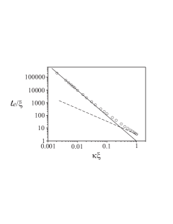
Figure 1: Numerical minimization of the variational equation (13) with respect to $\ell_{e}$: log-log plot of the renormalized persistence length, $\ell_{e}/\xi$, vs. the renormalized Debye parameter, $\kappa\xi$ (where $\xi$ is the electrostatic blob size). The solid line denotes the function $\ell_{e}=\frac{1}{\xi\kappa^{2}}$ while the broken line is proportional to $\kappa^{-1}$.

From Eq. (26), we can approximate the entropy per electrostatic blob by

$$\frac{n}{N}\beta(F_{0}-F_{\mathrm{uv}})\simeq-\frac{3}{\sqrt{2}}\left(\frac{\xi}{\ell_{e}}\right)^{1/2}$$ (32)

in the limit $\ell_{e}/\xi\rightarrow\infty$, which is the low-screening limit. Obviously, this limiting formula is different from the result found by Barrat and Joanny for the entropy, $\frac{n}{N}\beta F_{0}\simeq\ln(\ell_{e}/\xi)$ [see Eq. (7) of Ref. Barrat ]. This different dependence of the entropy on $\ell_{e}$ is the sole reason for their different scaling of the persistence length, resulting in $\ell_{e}\sim\kappa^{-1}$.

The interaction term equation (4) is more difficult to evaluate. The two terms cannot be computed separately because of a cancellation of divergences. To make analytical progress, we assume the result (31) to be valid and replace $\ell_{e}$ by $1/(\xi\kappa^{2})$ in the first two terms of equation (4). We then look at the limit $\kappa\xi\rightarrow 0$. We find numerically for the leading term

$$\frac{n}{N}\beta\langle\mathcal{H}_{\mathrm{int}}\rangle_{0}\simeq-\ln(\kappa\xi)$$ (33)

It corresponds to the electrostatic energy of the blob in a cylindrical geometry and diverges logarithmically when $\kappa$ goes to 0. This term is independent of the electrostatic persistent length. To find the next leading term, we calculate the asymptotic behavior of the derivative of $\frac{n}{N}\beta\langle\mathcal{H}_{\mathrm{int}}(\ell_{e},\kappa)\rangle_{0}$ with respect to $\ell_{e}$ and then assume the KK law. As is visualized in Figure 2, we find

$$\frac{n}{N}\beta\xi\left.\frac{\partial\langle\mathcal{H}_{\mathrm{int}}\rangle_{0}}{\partial\ell_{e}}\right|_{\ell_{e}=(\kappa^{2}\xi)^{-1}}\sim-(\kappa\xi)^{3}+\mathcal{O}((\kappa\xi)^{5})$$ (34)

Keeping the first terms of the asymptotic expansion of $\partial F_{\mathrm{var}}/\partial\ell_{e}$, we thus get

$$\frac{\partial F_{0}}{\partial\ell_{e}}+\left.\frac{\partial\langle\mathcal{H}_{\mathrm{int}}\rangle_{0}}{\partial\ell_{e}}\right|_{\ell_{e}=(\kappa^{2}\xi)^{-1}}\sim\frac{\xi^{1/2}}{\ell_{e}^{3/2}}-\kappa^{3}\xi^{2}=0$$ (35)

and thus recover Eq. (31) in the asymptotic limit $\kappa\xi\rightarrow 0$ (within a numerical coefficient of the order of unity) in a self-consistent way.

Besides this asymptotic but cumbersome way, it is also possible to find the leading term in $(\kappa\ell_{e})^{-1}$ for the interaction term by using an approximated structure factor for the semi-flexible chain Barrat . Starting from Eq. (4), we see that

$$\beta\langle\mathcal{H}_{\mathrm{int}}\rangle_{0} = \frac{L\ell_{B}}{A^{2}}\int_{0}^{\infty}\mathrm{d}s\int\frac{\mathrm{d}^{3}\mathbf{q}}{(2\pi)^{3}}\frac{4\pi}{\kappa^{2}+\mathbf{q}^{2}}\left\langle\mathrm{e}^{\imath\mathbf{q}|\mathbf{r}(s)-\mathbf{r}(0)|}\right\rangle_{0}$$ (36)

$$= \frac{L\ell_{B}}{2A^{2}}\int\frac{\mathrm{d}^{3}\mathbf{q}}{(2\pi)^{3}}\frac{4\pi}{\kappa^{2}+q^{2}}S_{0}^{\infty}(q)$$

where the structure factor, $S_{0}^{\infty}(q)$, of an infinite chain computed using the variational Hamiltonian, $\mathcal{H}_{0}$, is given by

$$S_{0}^{\infty}(q)=2\int_{0}^{\infty}\mathrm{d}s\left\langle\mathrm{e}^{\imath\mathbf{q}|\mathbf{r}(s)-\mathbf{r}(0)|}\right\rangle_{0}$$ (37)

In the limit $\ell_{e}/\xi\rightarrow\infty$, the chain can be viewed as a semi-flexible chain made up of $N/n$ rods of length $\xi$ and of persistence length $\ell_{e}$. We thus neglect the internal blob structure. We can use an interpolating formula for the polyelectrolyte structure factor, $S_{0}^{\infty}(q)=(1+q\ell_{e})/(q^{2}\ell_{e})$ which exhibits the correct limiting behaviour for small momenta in $1/(q^{2}\ell_{e})$ and for large momenta in $1/q$ desCloiseaux . Using a upper cutoff at $q\simeq\xi^{-1}$ in Eq. (36), we easily find

$$\frac{n}{N}\beta\langle\mathcal{H}_{\mathrm{int}}\rangle_{0}\simeq-\frac{1}{2}\ln(\kappa\xi)+\frac{\pi}{4}\frac{1}{\kappa\ell_{e}}+\mathcal{O}\left(\frac{1}{(\kappa\ell_{e})^{2}}\right)$$ (38)

Taking a derivative with respect to $\ell_{e}$ and inserting the KK scaling Eq.(31), we recover Eq. (34). Hence, we note that the $\kappa^{-2}$ dependence of $\ell_{e}$ comes directly from the balance between the entropy of the chain in equation (32) and the electrostatic energy in equation (38) in the limit of weak screening.

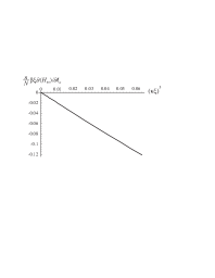
Figure 2: Numerical check of Eq. (34). The first derivative of the interaction term per electrostatic blob, $\frac{n}{N}\beta\xi\partial\langle\mathcal{H}_{\mathrm{int}}\rangle_{0}/\partial\ell_{e}|_{\ell_{e}=(\kappa^{2}\xi)^{-1}}$, decreases as $-(\kappa\xi)^{3}$ when $\ell_{e}$ is assumed to follow the KK law, $\ell_{e}\simeq(\kappa^{2}\xi)^{-1}$.

5 Stiff polyelectrolytes

In the persistent regime, for stiff and strongly charged polymers, $\ell_{0}\ell_{B}/A^{2}>1$, and at small screening, $\ell_{0}\ell_{B}/A^{2}>(\ell_{0}\kappa)^{2}$, the above variational kernel must be modified. According to OSF theory, which is based on the electrostatic contribution to the energy of a uniformly bent rod, the electrostatic monomer-monomer interactions are already relevant on length scales comparable to the bare persistent length, leading to an effective persistent length given by equation (2). However, Barrat and Joanny have shown within a quadratic perturbation treatment that the persistence length is in fact scale-dependent and that the OSF prediction corresponds to the large-scale limit Barrat . Since all these calculations are perturbative and only valid for weakly bent chains, it is interesting to have a variational determination of the effective persistent length $\ell_{p}=\ell_{0}+\ell_{e}$ in this persistent regime. The first choice would be the WLC model with a variable persistence length. Treating the persistence length $\ell_{p}$ as a variational parameter, the tangent-tangent correlation function and the squared monomer separation are given by Eqs. (15) and (16) where $\ell_{0}$ is replaced by $\ell_{p}$. For an infinite chain, $N\rightarrow\infty$, a Gaussian Hamiltonian which leads to these equations is Eq. (7) with $\ell_{B}/A^{2}=0$ and $\ell_{p}$ instead of $\ell_{0}$. However, this variational Hamiltonian with $\ell_{p}$ as the variational parameter does not work because the variational entropic free energy diverges at small length scales

$$\beta F_{\mathrm{wlc}}=-\frac{3L}{2}\int_{-\infty}^{\infty}\frac{\mathrm{d}\omega}{2\pi}\ln\left[\frac{\ell_{p}}{\ell_{0}}\frac{2}{\ell_{0}^{2}\omega^{2}(1+\ell_{p}^{2}\omega^{2})}\right]$$ (39)

since the integrand behaves like $\ln(\ell_{0}\ell_{p}\omega^{4})$ when $\omega\rightarrow\infty$. This divergence depends on the variational parameter, and therefore, a variational approach based on such a Hamiltonian is ill-defined. This fact is reflected by Monte-Carlo simulations and perturbative calculations for the tangent-tangent correlation function of a charged chain : at small length scales, the decay of this correlation function is given by the bare (mechanical) persistence length, and only at larger length scales one finds a crossover to the electrostatic persistence Barrat . This can be described by a scale-dependent persistence length $\ell_{p}(\omega)=\ell_{0}+\ell_{e}(\omega)$ where $\ell_{e}(\omega)\simeq 0$ for $\omega\rightarrow\infty$ and $\ell_{e}(\omega)\simeq\ell_{\mathrm{OSF}}$ for $\omega\rightarrow 0$ which leads to a tangent-tangent correlation with the limiting behaviours

$$\langle\mathbf{\dot{r}}(s)\mathbf{\dot{r}}(0)\rangle\simeq\left\{\begin{array}[]{lcr}1-\frac{|s|}{\ell_{0}}&\mathrm{for}&|s|<s_{c}\\ \exp\left(-\frac{|s|}{\ell_{0}+\ell_{\mathrm{OSF}}}\right)&\mathrm{for}&|s|>s_{c}\end{array}\right.$$ (40)

where the crossover contour length $s_{c}$ has been determined in Ref. Barrat and is

$$s_{c}\simeq\frac{1}{\kappa\sqrt{1+\ell_{\mathrm{OSF}}/\ell_{0}}}$$ (41)

It transpires that the variational correlation function has to be chosen in accord with these limits. A simple and continuous choice for the tangent-tangent correlation function which fulfills Eq. (40) is

$$\langle\mathbf{\dot{r}}(s)\mathbf{\dot{r}}(0)\rangle_{0} = B\exp\left(-\frac{|s|}{\ell_{e}+\ell_{0}}\right)$$

$$+ (1-B)\exp\left[-|s|\frac{\ell_{e}+(1-B)\ell_{0}}{\ell_{0}(\ell_{e}+\ell_{0})(1-B)}\right]$$

where $\ell_{e}$ is the variational parameter and the factor $B$ is chosen such as to satisfy continuity

$$B=\exp\left[-\frac{\ell_{e}}{\kappa\sqrt{\ell_{0}}(\ell_{e}+\ell_{0})^{3/2}}\right]$$ (43)

Hence, the crossover $s_{c}=\sqrt{\ell_{0}}/(\kappa\sqrt{\ell_{e}+\ell_{0}})$ depends on the variational parameter. The case of a neutral semi-flexible polymer is recovered by taking $s_{c}\to\infty$ (which implies $B=0$) in Eq. (5). The tangent-tangent correlation function is plotted in Figure 3 for $\kappa\ell_{0}=1$ and $\ell_{e}=10\ell_{0}$.

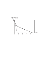
Figure 3: Log plot of the variational tangent-tangent correlation function vs. $\tilde{s}=s/\ell_{0}$ [see Eq. (5)]. The broken lines are the two asymptotic behaviours given by Eq. (40). The parameter values are $\kappa\ell_{0}=1$ and $\tilde{\ell}_{e}=10$

The Fourier transform, defined in Eq. (21), is easily computed

$$h(\omega) = 2B\frac{\ell_{e}+\ell_{0}}{1+(\ell_{e}+\ell_{0})^{2}\omega^{2}}$$

$$+ \frac{2(1-B)^{2}(\ell_{e}+\ell_{0})}{\ell_{e}+(1-B)\ell_{0}}\frac{\ell_{0}}{1+\left[\frac{(\ell_{e}+\ell_{0})(1-B)\ell_{0}}{\ell_{e}+(1-B)\ell_{0}}\right]^{2}\omega^{2}}$$

Following the lines of Section 3, we obtain for the entropy

$$\beta(F_{0}-F_{\mathrm{n}}) = -\frac{3L}{2}\int_{-\infty}^{\infty}\frac{\mathrm{d}\omega}{2\pi}\ln\left[\frac{1}{2\ell_{0}}(1+\ell_{0}^{2}\omega^{2})h(\omega)\right]$$

$$= -\frac{3N}{2(\tilde{\ell}_{e}+1)}\left[\tilde{\ell}_{e}+1-\frac{\tilde{\ell}_{e}}{1-B}\right.$$

$$+ \left.\frac{\sqrt{(1-B+\tilde{\ell}_{e})(1-B+B\tilde{\ell}_{e})}}{\sqrt{\tilde{\ell}_{e}+1}(1-B)}\right]$$

where $\tilde{\ell}_{e}$ is the adimensional electrostatic persistence length

$$\tilde{\ell}_{e}=\frac{\ell_{e}}{\ell_{0}}$$ (46)

and

$$\beta F_{\mathrm{n}}=\frac{3L}{2}\int_{-\infty}^{\infty}\frac{\mathrm{d}\omega}{2\pi}\ln\left[\frac{1}{2}\omega^{2}\ell_{0}^{2}(1+\ell_{0}^{2}\omega^{2})\right]$$ (47)

is the entropy of a neutral semi-flexible polymer. The elastic term is

$$\beta\langle\mathcal{H}_{\mathrm{el}}\rangle_{0} = \frac{3L}{4}\left(\frac{1}{\ell_{0}}-\ell_{0}\frac{\mathrm{d}^{2}}{\mathrm{d}s^{2}}\right)\langle\mathbf{\dot{r}}(0)\mathbf{\dot{r}}(0)\rangle_{0}$$ (48)

$$= -\frac{3N}{4}\frac{B\tilde{\ell}_{e}^{2}}{(1-B)(\tilde{\ell}_{e}+1)^{2}}$$

The electrostatic energy is found using Eq. (4) which yields

$$\beta\langle\mathcal{H}_{\mathrm{int}}\rangle_{0} = N\frac{\ell_{B}\ell_{0}}{A^{2}}\int_{0}^{\infty}\mathrm{d}x\left\{\sqrt{\frac{3}{\pi}}\frac{1}{\sqrt{f(x)}}-\kappa(\tilde{\ell}_{e}+1)\right.$$ (49)

$$\times \left.\mathrm{erfc}\left[\frac{\kappa(\tilde{\ell}_{e}+1)}{\sqrt{3}}\sqrt{f(x)}\right]\mathrm{e}^{\frac{1}{3}\kappa^{2}(\tilde{\ell}_{e}+1)^{2}f(x)}\right\}$$

where

$$f(x) = B(\mathrm{e}^{-x}-1+x)+\frac{(1-B)^{3}}{(\tilde{\ell}_{e}+1-B)^{2}}$$

$$\times \left(\mathrm{e}^{-x\frac{\tilde{\ell}_{e}+1-B}{1-B}}+x\frac{\tilde{\ell}_{e}+1-B}{1-B}-1\right)$$

The interaction term, Eq. (49), diverges logarithmically for small $x$ (rod-like divergence). In the computation, we thus subtract $N\frac{\ell_{B}\ell_{0}}{A^{2}}\sqrt{\frac{6}{\pi}}\int_{0}^{\infty}\frac{\mathrm{d}x}{x(1+x^{3})}$ which does not depend on the variational parameter.

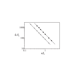
Figure 4: Numerical minimization of the variational equation free energy with respect to $\ell_{e}$ for stiff chains : log-log plot of the renormalized persistence length, $\ell_{e}/\ell_{0}$, vs. the renormalized Debye parameter, $\kappa\ell_{0}$ for two values of $\ell_{b}\ell_{0}/A^{2}$ : 2.25 (open circles) and 4 (full circles). Solid lines are the power law $\kappa^{-2}$.

The minimization of the variational free energy is done numerically and the result is plotted in Figure 4 for $\ell_{B}\ell_{0}/A^{2}=2.25$ and 4. We observe that the OSF result is recovered with a decrease $\tilde{\ell}_{e}\sim\kappa^{-2}$ in both cases.

We should add that we find the persistence length to depend on the charge parameter $\ell_{B}\ell_{0}/A^{2}$ as $\tilde{\ell}_{e}\sim(\ell_{B}\ell_{0}/A^{2})^{2}$ which is different from the linear dependence found by OSF [Eq. (2)]. At this point we have no clear interpretation for this discrepancy. Because of numerical limitations, we could calculate the effective persistence length only for moderate values of the charge parameter up to $\ell_{B}\ell_{0}/A^{2}=8$, which is the range of parameters found for fully charged flexible (synthetic) polymers. This parameter range is thus very far from the value $\ell_{B}\ell_{0}/A^{2}=150$ used in the simulations by Barrat and Joanny. An explanation could be that close to the crossover $\ell_{B}\ell_{0}/A^{2}=1$, the correction, $\varphi$, to the OSF law according to

$$\tilde{\ell}_{e}=\frac{1}{4}\frac{\ell_{B}\ell_{0}}{A^{2}}\frac{1}{(\kappa\ell_{0})^{2}}\,\varphi\left(\kappa\ell_{0},\frac{\ell_{B}\ell_{0}}{A^{2}}\right)\quad\mathrm{with}\quad\varphi(0,\infty)=1$$ (51)

is very large. This point will be studied by suitable simulations in the future.

6 Discussion

In this section, we discuss the results of Section 3 and compare our approach to those of Barrat and Joanny Barrat , Schmidt Schmidt , Ha and Thirumalai Thirumalai1 ; Thirumalai2 and Muthukumar et al. Muthu2 ; Ghosh . All these works are variational approaches with only one variational parameter. However, as explained in the Introduction, we shall distinguish between two types of works, according to the physical interpretation of this parameter. In Ref. Muthu2 ; Ghosh , it reflects the swelling behaviour at large length scales and reproduce the correct swelling law as a function of $N$. This variational parameter is then not interpreted as the true mechanical persistence length. In the other references Schmidt ; Barrat ; Thirumalai1 ; Thirumalai2 , the variational parameter is interpreted as a persistence length and the swelling behaviour at large scales is not considered. Our variational calculation belongs to this category. We show that, in this case, the persistence length is finite for an infinite chain, $N\to\infty$.

As mentioned in Section 3, our variational calculation is similar to Barrat and Joanny calculation. They find the result Eq. (38) for the interaction term, by approximating the structure factor of a polyelectrolyte and by using an upper cutoff at $q\simeq\xi^{-1}$. Hence they “smooth” electrostatic interactions inside the electrostatic blobs. This approximation is valid only in the limit $\ell_{e}/\xi\to\infty$, i.e. in the limit of weak screening. However, using the same cutoff at $q\simeq\xi^{-1}$ in the calculation of the entropic term, they find $\beta F_{0}\simeq\frac{N}{n}\ln(\ell_{e}/\xi)$, which is different from our result, Eq. (26), and leads to their law $\ell_{e}\simeq\kappa^{-1}$. Evidently, this un-controlled cutoff leads to the correct result for the interaction term but not for the entropy.

Schmidt Schmidt use a different variational formulation, where the elastic energy is calculated for a stretched random flight chain and the electrostatic energy is approximated using an hybrid rod-coil model. This leads to a weaker dependence than $\kappa^{-2}$ for $\ell_{e}$ but which does not follow a power law and tends to vary as $\kappa^{-1}$ at high ionic strength. However, $\ell_{e}$ increases with the contour length and seems to diverge for $N\to\infty$. Moreover, as carefully explained in Ref. Schmidt , this calculation does not apply to the low ionic strength limit in view of the approximations made.

Ha and Thirumalai Thirumalai1 ; Thirumalai2 use the same variational squared monomer separation, Eq. (20), but follow the uniform expansion method, first developed by Edwards and Singh Singh ; DE . This perturbative variational method is performed on the mean-square end-to-end distance, $\langle R^{2}\rangle$. It consists in calculating self-consistently the persistence length by requiring $\langle R^{2}\rangle-\langle R^{2}\rangle_{0}$ to be zero at first order in $\ell_{0}\ell_{B}/A^{2}$. This method has proved to be powerful in the calculation of the Flory exponent for the end-to-end distance of neutral polymers. For our issue, Yethiraj shows that in the limit $L/\ell_{e}\to\infty$ the Gibbs-Bogoliubov approach and the uniform expansion method applied to the end-to-end distance lead to the same self-consistent equation Yethiraj . Clearly, both variational approaches lead to similar results for a given observable. The important point is to carefully consider, in both approaches, the behaviour at small length scales.

This method is applied both in the limit $\ell_{0}\ell_{B}/A^{2}\ll 1$ and at the so-called non-asymptotic limit, $\ell_{b}\ell_{0}/A^{2}\sim 1$, when the blob size is of the order of the bare persistent length $\xi\simeq\ell_{0}$ Thirumalai1 ; Thirumalai2 . In the first case, they find the KK result Thirumalai2 but in their calculation they approximate the chain by a rod on a scale of the order of $\ell_{e}$ (thus factorizing the statistical weights, see Eq. (2.18) in Ref. Thirumalai2 ). Moreover they skip a priori the integrals on long length scales, $s>\ell_{e}$, in the calculation, arguing that they lead to an effective excluded-volume interaction. Hence, the dependence of the persistence length on $N$ is eliminated. In the non-asymptotic limit, Ha and Thirumalai use a simple Gaussian variational weight used for neutral and flexible polymers and find $\ell_{e}\simeq(\ell_{0}\ell_{B}/A^{2})^{1/2}\kappa^{-1}$. However, as we explained in the preceding section, this choice of Hamiltonian leads to a divergent entropic term. To circumvent this problem, the evaluation of the statistical averages is done by imposing a lower cutoff at $q\simeq\ell_{e}^{-1}$. We believe that this approximation leads to the scaling $\ell_{e}\sim\kappa^{-1}$.

As shown by Muthukumar et al. Muthu2 ; Ghosh the uniform expansion method applied to $\langle R^{2}\rangle$ cannot be used to infer the scaling of the persistent length. Indeed, to make the variational equation tractable (see Eq. (3.38) of Ref. Muthu2 ), they approximate the variational kernel $h(\omega)$ (noted $l_{1}(q)$ in their paper) by the effective persistence length $\ell_{e}$ [valid in the limit $\omega\to 0$, as it can be seen from Eq. (22)] and they evaluate the integrand for $\omega\simeq 2\pi/L$. Hence, these approximations are valid in the limit of large length scales and this method is powerful to get the large scale behaviour : they indeed recover the swelling exponent in the infinite limit $N\to\infty$, $\langle R^{2}\rangle\sim N^{6/5}$ due to effective excluded volume interactions (which are the screened electrostatic interactions if $\kappa^{-1}$ is non zero). But the extrapolated persistence length from $\langle R^{2}\rangle\sim\ell_{p}N$ is $\ell_{p}\sim N^{1/5}$, and does not correspond to the mechanical persistence length. In this approach, the small scale behaviour is, in a sense, averaged out, and all the electrostatics contribute to excluded volume interactions.

The uniform expansion can be used to calculate next-leading corrections in an asymptotic expansion of the persistence length $\ell_{e}$ of the order of $\mathcal{O}((\kappa\xi)^{-1}$. But in this case, it must be applied to to the observable conjugated to the variational parameter, $\ell_{e}$, namely the bending energy $\int\mathrm{d}s\,\mathbf{\ddot{r}}^{2}(s)$, and not to the end-to-end distance. This could be valuable near the crossover, $\kappa\xi\sim 1$, between the Gaussian-persistent regime and the Gaussian regime.

In two recent papers Everaers ; Nguyen , simulations on long polyelectrolytes (up to $N=4096$) show a behaviour consistent with the KK formula (5). Discrimination between $\ell_{e}\sim\kappa^{-1}$ and $\ell_{e}\sim\kappa^{-2}$ is clearly seen only for very long polymers which is one of the reason why the available experimental data are not very conclusive on this point. Furthermore, in experiments there are other effects such as counterion condensation and electrostatic correlations which are not included on the Debye-Hückel level.

7 Concluding remarks

Our calculation is done within three important assumptions : i) we study an infinitely long chain ($N\to\infty$), ii) we do not consider excluded volume interactions at large length scales and, iii) we take into account electrostatic interactions at the linear level [a Debye-Hückel potential is used in equation (7)]. Within these assumptions, we show that the electrostatic contribution to the persistence length, $\ell_{e}$, is proportional to $\kappa^{-2}$, both for flexible (KK result), Eq. (5), and stiff polymers (OSF result), Eq. (2). This result is very robust (we tried a different variational choice shown in the Appendix which leads to the same formula) and is in contradiction with several theoretical papers where a $\kappa^{-1}$ dependence was found for flexible polymers. We show that this difference can be explained by the use of a cutoff at small length scales in those works.

Obviously, a full comparison with experimental measurements on very long chains would be necessary to validate this variational approach. Comparison with experimentally determined persistence lengths of polyelectrolytes has been done in several articles Schmidt ; Netz ; Everaers . Essentially, some experimental papers raised some doubts about the validity of the OSF result and proposed a law in $\ell_{e}\sim\kappa^{-1}$ Reed . This law has been found using approximate formulas for the radius of gyration to deduce the persistence length, and the discrepancy can be due to an incomplete theory used in the data analysis, as shown by Ghosh et al. Ghosh .

More importantly, a deviation from the Debye-Hückel-type theory used in our paper arises due to non-linear electrostatic effects. For highly charged polymers (especially in the persistent regime), the renormalization of the bare charge of the chain associated with the condensation of counterions (known as the Manning condensation Manning ) also influences the dependence of $\ell_{e}$ on the Debye screening length. A recent study of this effect using a variational approach applied to a charged cylinder Netz2 shows that the effective charge density along the polymer follows $A\sim\kappa^{-0.3}$ which would lead to a modified power law $\ell_{e}\sim\kappa^{-1.4}$. We are currently studying this effect for a semi-flexible polyelectrolyte.

Finally, we hope that this simple variational approach can be extended to the issue of the electrostatic persistent length of polyelectrolytes in semi-dilute solutions by combining this type of variational approach with the random-phase approximation to account for monomer-monomer correlations and screening induced by neighboring polymers Muthu2 ; Ghosh ; Yethiraj ; Donley1 ; Donley2 .

Appendix

In this appendix, we show that the KK result is also found with a piece-wise continuous tangent-tangent correlation function which exhibits the same behaviour as the modified WLC model at the asymptotic limits $|s|\ll n^{1/2}\ell_{e}$ and $|s|\gg n^{1/2}\ell_{e}$. The advantage of this formulation is that the interaction term, Eq. (4) is easily computed, and therefore we can show that the large-scale term in the integrals is negligible in the determination of the persistence length. Moreover, we thus prove that our result for the salt-dependence of the persistence length is robust and insensitive to the detailed choice of the variational correlation function.

Our variational choice for the squared monomer separation is

$$G_{\mathrm{pw}}(s)=\left\{\begin{array}[]{lcr}\ell_{0}|s|+\frac{s^{2}}{n}\left(1-\frac{1}{3}\frac{|s|}{n^{1/2}\ell_{e}}\right)&\mathrm{for}&|s|<n^{1/2}\ell_{e}\\ \left(\ell_{0}+\frac{\ell_{e}}{n^{1/2}}\right)|s|-\frac{\ell_{e}^{2}}{3}&\mathrm{for}&|s|>n^{1/2}\ell_{e}\end{array}\right.$$ (52)

where “pw” refers to piece-wise. For $|s|<n^{1/2}\ell_{e}$, the first line of Eq. (52) is a sum of a linear term (Gaussian behaviour at small length scales) and a term which imposes almost a rod-like behaviour for arc lengths ranging in $n\ell_{0}<|s|<n^{1/2}\ell_{e}$. These linear and quadratic terms in the first line of Eq. (52) are of equal magnitude for $s=n\ell_{0}$, the number of monomers in a Gaussian blob at the onset of the persistent behaviour. For $|s|>n^{1/2}\ell_{e}$, the statistics is again Gaussian, as expected for a semi-flexible chain at large length scales.

The tangent-tangent correlation function is thus computed through $\langle\mathbf{\dot{r}}(s)\mathbf{\dot{r}}(0)\rangle_{\mathrm{pw}}=\frac{1}{2}G_{\mathrm{pw}}^{\prime\prime}(s)$

$$\langle\mathbf{\dot{r}}(s)\mathbf{\dot{r}}(0)\rangle_{\mathrm{pw}}=\left\{\begin{array}[]{lcr}\ell_{0}\delta(s)+\frac{1}{n}\left(1-\frac{|s|}{n^{1/2}\ell_{e}}\right)&\mathrm{for}&|s|<n^{1/2}\ell_{e}\\ 0&\mathrm{for}&|s|>n^{1/2}\ell_{e}\end{array}\right.$$ (53)

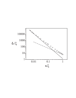
Figure 5: Same plot as in Figure 1 with a piece-wise variational squared monomer separation function $G_{\mathrm{pw}}$

.

The function $h$, defined in Eq. (21), is then

$$h_{\mathrm{pw}}(\omega)=\ell_{0}\left[1+\frac{2}{\ell_{e}\xi}\frac{1-\cos(\omega n^{1/2}\ell_{e})}{n\omega^{2}}\right]$$ (54)

We find exactly the same elastic part, Eq. (23), as in the modified WLC model and for the entropy term we have

$$\beta\left(F_{\mathrm{pw}}-F_{\mathrm{uv}}\right)=-\frac{\xi}{4\pi\ell_{e}}\frac{N}{n}\int_{0}^{\infty}\mathrm{d}x\ln\left(1+2\frac{\ell_{e}}{\xi}\frac{1-\cos x}{x^{2}}\right)$$ (55)

where $F_{\mathrm{uv}}$ is given in Eq. (25). The interaction term is found to be

$$\frac{n}{N}\beta\langle\mathcal{H}_{\mathrm{int}}\rangle_{\mathrm{pw}} = \int_{0}^{1}\mathrm{d}x\left\{\sqrt{\frac{6}{\pi}}\frac{1}{\sqrt{x\xi/\ell_{e}+x^{2}-x^{3}/3}}\right.$$

$$- \left.\kappa\ell_{e}\exp\left[\frac{(\kappa\ell_{e})^{2}}{6}\left(\frac{x\xi}{\ell_{e}}+x^{2}-\frac{x^{3}}{3}\right)\right]\right.$$

$$\times \left.\mathrm{erfc}\left[\frac{\kappa\ell_{e}}{\sqrt{6}}\left(\frac{x\xi}{\ell_{e}}+x^{2}-\frac{x^{3}}{3}\right)^{1/2}\right]\right\}$$

$$+ \frac{6}{\kappa(\xi+\ell_{e})}\exp\left[\kappa^{2}\ell_{e}\xi\left(\frac{1}{6}+\frac{\ell_{e}}{9\xi}\right)\right]$$

$$\times \mathrm{erfc}\left[\kappa\sqrt{\ell_{e}\xi}\left(\frac{1}{6}+\frac{\ell_{e}}{9\xi}\right)^{1/2}\right]$$

The numerical minimization of Eq. (13) is shown in Fig. 5 and shows that the KK result is also found with this variational approach.

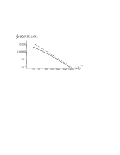
Figure 6: First derivative of the interaction term per electrostatic blob,$\frac{n}{N}\beta\xi\partial\langle\mathcal{H}_{\mathrm{int}}\rangle_{0}/\partial\ell_{e}|_{\ell_{e}=(\kappa^{2}\xi)^{-1}}$, vs. $\kappa\xi$ when $\ell_{e}$ is set to follow the KK law, $\ell_{e}\simeq(\kappa^{2}\xi)^{-1}$ in a log-log scale. The dotted line is the power law $(\kappa\xi)^{3}$.

We have checked numerically that the entropy per electrostatic blob given by Eq. (55) has the same dependence in $-\sqrt{\xi/\ell_{e}}$ for $\ell_{e}/\xi\to\infty$ as for the modified WLC model [Eq. (26)]. The last term of equation (Appendix) corresponding to the large scale behaviour, i.e. for $|s|>n^{1/2}\ell_{e}$, can easily be evaluated using the saddle point expansion and varies like $\sim(\kappa\ell_{e})^{-2}$. By applying exactly the same routine as in Section 3, we show (Fig. 6)

$$\frac{n}{N}\beta\langle\mathcal{H}_{\mathrm{int}}\rangle_{0}+\ln(\kappa\xi)\simeq\frac{1}{\kappa\ell_{e}}$$ (57)

which yields the same result as in Section 3. We thus note that the electrostatic energy at small length scales, $|s|<n^{1/2}\ell_{e}$, is larger in the limit $\ell_{e}/\xi\to\infty$ and governs the dependence of $\ell_{e}$ with $\kappa$.

- (1) S. Förster, M. Schmidt, Adv. Pol. Sci., 120, 51 (1995).
- (2) J.-L. Barrat, J.-F. Joanny, Adv. Chem. Phys., 94, 1 (1996).
- (3) R.R. Netz, D. Andelman, Physics Reports, 380, 1 (2003).
- (4) R. Golestanian, M. Kardar, T.B. Liverpool, Phys. Rev. Lett. 82, 4456 (1999).
- (5) T.T. Nguyen, I. Rouzina, B.I. Shklovskii, Phys. Rev. E 60, 7032 (1999).
- (6) G. Ariel and D. Andelman, Europhys. Lett. 61, 67 (2003).
- (7) U. Micka, K. Kremer, Phys. Rev. E, 54, 2653 (1996).
- (8) M.J. Stevens and S.J. Plimpton, Eur. Phys. J. B 2 341 (1998).
- (9) R. Everaers, A. Milchev, V. Yamakov, Eur. Phys. J. E, 8, 3 (2002).
- (10) T.T. Nguyen, B.I. Shklovskii, Phys. Rev. E, 66, 021801 (2002).
- (11) M. Ullner and C.E. Woodward, Macromolecules 35, 1437 (2002).
- (12) M. Schmidt, Macromolecules, 24, 5361 (1991).
- (13) J.-L. Barrat, J.-F. Joanny, Europhys. Lett., 24, 333 (1993).
- (14) D. Bratko, K.A. Dawson, J. Chem. Phys., 99, 5352 (1993).
- (15) H. Li, T.A. Witten, Macromolecules, 28, 5921 (1995).
- (16) B.-Y. Ha, D. Thirumalai, Macromolecules, 28, 577 (1995).
- (17) R.R. Netz, H. Orland, Eur. Phys. J. B, 8, 81 (1999).
- (18) B.-Y. Ha, D. Thirumalai, J. Chem. Phys., 110, 7533 (1999).
- (19) A.R. Khokhlov, K.A. Khachaturian, Polymer, 23, 1742 (1982).
- (20) T. Odijk, J. Polym. Sci., 15, 477 (1977).
- (21) J. Skolnick, M. Fixman, Macromolecules, 10, 944 (1977).
- (22) P.-G. de Gennes, P. Pincus, R.M. Velasco, F. Brochard, J. Phys. (Paris), 37, 1461 (1976).
- (23) P. Pfeuty, J. Phys. (Paris), 39, C2-149 (1978).
- (24) T.B. Liverpool, M. Stapper, Eur. Phys. J. E, 5, 359 (2001).
- (25) P.L. Hansen and R. Podgornik, J. Chem. Phys. 114, 8637 (2001).
- (26) S.F. Edwards, P. Singh, J. Chem. Soc. Farady Trans. II, 75, 1001 (1979).
- (27) M. Doi, S.F. Edwards, The Theory of Polymer Dynamics (Oxford University Press, Oxford 1986).
- (28) B. Jönsson, C. Peterson and B. Söderberg, J. Phys. Chem., 99, 1251 (1995).
- (29) M. Muthukumar, J. Chem. Phys., 105, 5183 (1996).
- (30) K. Ghosh, G.A. Carri, M. Muthukumar, J. Chem. Phys., 115, 4367 (2001).
- (31) A. Yethiraj, J. Chem. Phys., 108, 1184 (1998).
- (32) J.P. Donley, J. Rudnick, A.J. Liu, Macromolecules, 30, 1188 (1997).
- (33) J.P. Donley, J. Chem. Phys., 116, 5315 (2002).
- (34) T. Hofmann, R.G. Winkler, P. Reineker, J. Chem. Phys., 118, 6624 (2003).
- (35) J.B. Lagowski, J. Noolandi, B. Nickel, J. Chem. Phys., 95, 1266 (1991).
- (36) J. des Cloiseaux, J. Jannink, Les Polymères en Solution: leur Modélisation et leur Structure (Les Editions de Physique, Paris, 1987).
- (37) W.F. Reed, S. Ghosh, G. Medjahdi, J. François, Macromolecules, 24, 6189 (1991).
- (38) G.S. Manning, J. Chem. Phys., 51, 924 (1969).
- (39) R.R. Netz, H. Orland, Eur. Phys. J. E, 11, 301 (2003).