Generation of Squeezed States of Nanomechanical Resonators by Reservoir Engineering

Abstract

An experimental demonstration of a non-classical state of a nanomechanical resonator is still an outstanding task. In this paper we show how the resonator can be cooled and driven into a squeezed state by a bichromatic microwave coupling to a charge qubit. The stationary oscillator state exhibits a reduced noise in one of the quadrature components by a factor of 0.5 - 0.2. These values are obtained for a 100 MHz resonator with a Q-value of 10⁴ to 10⁵ and for support temperatures of T $\approx$ 25 mK. We show that the coupling to the charge qubit can also be used to detect the squeezed state via measurements of the excited state population. Furthermore, by extending this measurement procedure a complete quantum state tomography of the resonator state can be performed. This provides a universal tool to detect a large variety of different states and to prove the quantum nature of a nanomechanical oscillator.

I Introduction

With fabrication of nanomechanical resonators with fundamental frequencies from 100 MHz up to 1 GHz Cleland (2003); Cleland and Roukes (1996); Huang et al. (2003) the demonstration of their quantum nature, in particular, the creation of non-classical states of these mesoscopic systems, have attracted a lot of interest Carr et al. (2001); Blencowe and Wybourne (2000a); Armour et al. (2002); Irish and Schwab (2003); Eisert et al. (2003). Apart from the fundamental interest in the study of these systems, nanomechanical resonators are also of great importance for technical applications. While micron-sized cantilevers are already used to perform atomic force measurements, their noise properties which set the limits for the sensitivity of force detection Braginsky and Khalili (1992); Sidles et al. (1995) can be improved by scaling them down to the nanometer regime. Residual thermal fluctuations can then be reduced to the quantum limit by active cooling schemes as proposed in Hopkins et al. (2003); Wilson-Rae et al. (2004); Martin et al. (2004).

A further reduction of the quantum fluctuations below the standard quantum limit can be achieved by squeezing the resonator mode. The idea to use squeezed states for measurements beyond the standard quantum limit Caves et al. (1980) appeared first in the context of the detection of gravitation waves. In principle it applies to any system where a weak classical force which has to be measured acts on a quantum-mechanical oscillator. The measurement consists of three stages. In the first stage one prepares the oscillator in a squeezed state, so that the dispersion of one of its quadratures is reduced below the quantum limit. Next, one allows the measured force to act on the oscillator. At last one measures the squeezed quadrature, without touching the other one. To apply the squeezing ideas to the nanomechanical systems, all three stages have to be implemented. In particular, for the third stage, one has to design a setup in which only one of the quadratures is being measured. In this paper we restrict ourselves to the first stage, i.e., the preparation of the squeezed state of a nanomechanical oscillator. We show that by coupling the oscillator to a Cooper Pair Box (Josephson qubit) and irradiating the system by bichromatic, phase coherent microwaves one can “cool” the oscillator down to the squeezed state.

We start by reminding the reader about the basics of squeezing and discuss two different ways to achieve it. Then we analyze the coupled CPB - oscillator system and show that the cooling into the squeezed state is feasible. At last we discuss possible ways to detect the squeezed state.

II Squeezed States and Reservoir Engineering

For a harmonic oscillator with a Hamiltonian $H=\hbar\nu\,a^{\dagger}a$, where $a$ and $a^{\dagger}$ are the usual creation and annihilation operators, a general class of Gaussian minimum-uncertainty squeezed states is defined by Walls and Milburn (1994)

$$|\alpha,\epsilon\rangle=\hat{D}(\alpha)\hat{S}(\epsilon)|0\rangle$$ (1)

Here $\hat{D}(\alpha)\!=\!\mathrm{exp}(\alpha a^{\dagger}-\alpha^{*}a)$ is a displacement operator, and $\hat{S}(\epsilon)\!=\!\mathrm{exp}(\frac{\epsilon^{*}}{2}a^{2}-\frac{\epsilon}{2}a^{{\dagger}2})$ denotes the squeezing operator. We refer to the state $|\epsilon\rangle\equiv|\alpha\!=\!0,\epsilon\rangle$ as the squeezed vacuum state. The absolute value of the complex number $\epsilon\!=\!re^{i\theta}$ is called the squeezing parameter. For these squeezed states the quadrature components, $X_{1,2}$, defined by $a=(X_{1}+iX_{2})e^{i\theta/2}$ fulfill the uncertainty relation $\Delta X_{1}\Delta X_{2}\geq\frac{1}{4}$, where the variance of one component, $\Delta X_{1}=e^{-r}/2$ is reduced below the standard quantum limit of 1/2, whereas the noise in the other component is enhanced, $\Delta X_{2}=e^{+r}/2$. This property can be exploited to improve the sensitivity of measurements. It is important to note that this asymmetric distribution of the noise is stationary only in a frame rotating with the frequency $\nu$ of the harmonic oscillator, since an initial squeezed state $|\epsilon\rangle$ evolves in time as $|\epsilon e^{-i2\nu t}\rangle$. Therefore, the error ellipse rotates in phase space with the oscillator frequency, $\nu$, as shown in Fig. 1.

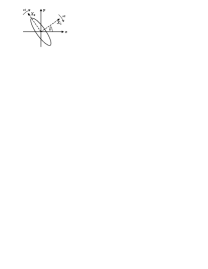
Figure 1: Representation of the squeezed state $|\,\epsilon\!=\!re^{i\theta}\rangle$ in phase space spanned by the dimensionless position and momentum coordinates. The error ellipse indicates the reduced/enhanced fluctuations for the quadrature components $X_{1}$/$X_{2}$.

There are several ways to generate a squeezed state of a harmonic oscillator. A familiar method in quantum optics Squ is to use a parametrically driven non-linear potential corresponding to the Hamiltonian

$$H=\hbar\nu a^{\dagger}a-i\hbar\lambda(a^{{\dagger}2}e^{-i\omega_{p}t}-a^{2}e^{i\omega_{p}t})\,.$$ (2)

By going to a rotating frame, i.e. transforming the time-dependence away and assuming a parametric pump field frequency $\omega_{p}=2\nu$, the Hamiltonian is simply given by $H_{\mathrm{I}}=i\hbar\lambda(a^{2}-a^{{\dagger}2})$. Starting from the ground state of the harmonic oscillator, $|0\rangle_{\mathrm{I}}$ the time evolution with $H_{\mathrm{I}}$ produces the squeezed state $|\epsilon\!=\!2\lambda t\rangle_{\mathrm{I}}$. The application of this method for mechanical resonators has been proposed in Ref. Blencowe and Wybourne (2000a), but the requirements, a sufficiently strong nonlinearity to overcome the losses, and an initial state close to the ground state, are not easily met.

A second method, which we will elaborate on below, is to “engineer” an appropriate coupling to the environment such that a dissipative dynamics drives the harmonic oscillator into a squeezed state, i.e.  we “cool” the oscillator mode to a squeezed state. This reservoir engineering has been first proposed in Ref. Cirac et al. (1993); Poyatos et al. (1996) in the context of ion traps, and has been experimentally implemented in part by the Ion Trap Group at NIST in Boulder Myatt et al. (2000). This reservoir engineering can be achieved, for example, by coupling the oscillator to a dissipative two level system (TLS), where the form of the coupling determines the stationary state.

The simplest (although trivial) example is provided by a reservoir which cools the oscillator to the ground state $|0\rangle$. We assume that the oscillator is coupled to a two-level system with ground and excited state $|g\rangle$, $|e\rangle$ according to the Hamiltonian $H_{\mathrm{I}}=g(a\sigma_{+}+a^{\dagger}\sigma_{-})$, where we use Pauli spin notation $\sigma_{+}\equiv|e\rangle\langle g|$ etc.. We furthermore assume that the two-level system decays from the excited state to the ground state with a rate $\Gamma$. The time evolution in the interaction picture is then described by the master equation

$$\frac{d\rho}{dt}=-i[H_{\mathrm{I}},\rho]+\frac{\Gamma}{2}\left(2\sigma_{-}\rho\sigma_{+}-\sigma_{+}\sigma_{-}\rho-\rho\sigma_{+}\sigma_{-}\right)\;.$$ (3)

For long times the system thus evolves to the steady state $\rho=|0\rangle\langle 0|\otimes|g\rangle\langle g|$ since $|0\rangle|g\rangle$ is a “dark state” of the system Hamiltonian, i.e. $H_{\mathrm{I}}|0\rangle|g\rangle=0$.

For a general Hamiltonian of the form $H_{\mathrm{I}}=\hat{F}\sigma_{+}+\hat{F}^{\dagger}\sigma_{-}$ where $\hat{F}$ is a function of $a$ and $a^{\dagger}$ only, the dynamics of master equation (3) “cools” the system into the state $\rho=|\psi\rangle\langle\psi|\otimes|g\rangle\langle g|$. The stationary oscillator state $|\psi\rangle$ is determined by $\hat{F}|\psi\rangle=0$. A squeezed vacuum state, $|\epsilon\!=\!re^{i\theta}\rangle$ obeys the relation

$$\left(a\cosh(r)+a^{\dagger}\sinh(r)e^{-i\theta}\right)|\epsilon\rangle=0\,,$$ (4)

and thus we choose $\hat{F}$ to be of the form  Cirac et al. (1993)

$$\hat{F}=g_{1}a+g_{2}e^{-i\theta}a^{\dagger}\,,$$ (5)

where $g_{1}$ and $g_{2}$ are related by $r\!=\!\mathrm{atanh}(g_{2}/g_{1})$. For a single trapped ion driven by laser light and decaying via spontaneous emission such a Hamiltonian, $H_{\rm I}$ with $\hat{F}$ given in Eq. (5) can be constructed by applying two laser beams, one detuned to the “red sideband” ($\omega=\omega_{ge}-\nu$) and a weaker one detuned to the “blue sideband” ($\omega=\omega_{ge}+\nu$) of the two-level transition frequency $\omega_{ge}$. This is illustrated in in Fig. 2. For a detailed explanation the reader is referred to the review article by Leibfried et al. Leibfried et al. (2003).

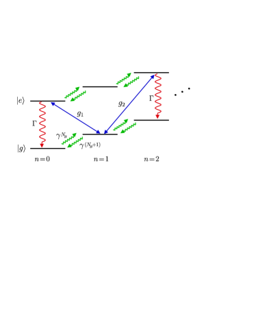
Figure 2: Coherent and incoherent processes as described by master equation  (6). The excitations of the qubit coherently decrease ($g_{1}$,“red sideband”) and increase ($g_{2}$,“blue sideband”) the phonon number of the oscillator. The energy of the excite state is then dissipated with the decay rate of the TLS, $\Gamma$. These two processes relax the system into the desired state, $\rho=|\epsilon,g\rangle\langle\epsilon,g|$ while the coupling to the thermal phonon bath, $\gamma$ thermalizes the oscillator state.

In the following section we show how such a Hamiltonian can be realized for a nanomechanical resonator coupled to a Cooper pair box, which plays the role of the dissipative two-level system  Martin et al. (2004).

For a mechanical resonator the coupling of the oscillator mode to the finite temperature phonon bath of the support has to be taken into account, leading to additional contributions in the master equation. As we discuss below, in the limit of high resonator frequencies where the rotating wave approximation (RWA) is valid the master equation is

$$\begin{split}\frac{d\rho}{dt}=-&i[H_{\rm I},\rho]+\frac{\Gamma}{2}\left(2\sigma_{-}\rho\sigma_{+}-\sigma_{+}\sigma_{-}\rho-\rho\sigma_{+}\sigma_{-}\right)\\ &+(N_{\mathrm{B}}+1)\frac{\gamma}{2}\left(2a\rho a^{\dagger}-a^{\dagger}a\rho-\rho a^{\dagger}a\right)\\ &+N_{\mathrm{B}}\frac{\gamma}{2}\left(2a^{\dagger}\rho a-aa^{\dagger}\rho-\rho aa^{\dagger}\right)\,.\end{split}$$ (6)

The new terms in the master equation describe the heating and dissipation of the resonator with rate $\gamma$, which relaxes to a thermal state with mean phonon occupation $\langle a^{\dagger}a\rangle=N_{\mathrm{B}}$. This will degrade the squeezing.

III The Model

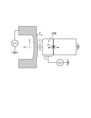
Figure 3: Setup: The mechanical resonator (thin, vertical bar) is biased by the voltage $V_{x}$ to achieve a coupling to the Cooper pair box (CPB) via the capacitance $C_{x}$. The state of the CPB can be controlled independently by the gate voltage, $V_{g}$ and the Josephson energy, $E_{J}$.

We consider a nanomechanical resonator which is placed close to a Cooper pair box (CPB) as shown in Fig. 3. Similar systems have been considered in the context of cooling Martin et al. (2004) and the generation of entangled states Armour et al. (2002). The energy spectrum of the CPB alone is controlled by the gate voltage, $V_{g}$ and the Josephson energy, $E_{J}$ Yu. Makhlin et al. (2001). To obtain a coupling between the two systems the voltage $V_{x}$ is applied on the resonator, leading to a position dependent interaction via the capacitance $C_{x}(x)$. The whole system is described by the Hamiltonian

$$H=\frac{(Q-Q_{g})^{2}}{2C_{\Sigma}}-E_{J}\cos(\phi)+\hbar\nu a^{{\dagger}}a\,.$$ (7)

Here $Q_{g}=C_{g}V_{g}+C_{x}V_{x}$ is the total gate charge, $C_{\Sigma}$ is the total capacitance of the island and $\nu$ is the frequency of the fundamental flexural mode of the resonator. We decompose the voltages into a sum of a constant and a time dependent part, $V_{i}=V_{i}^{0}+V_{i}(t)$ and therefore $Q_{g}=2e(n_{g}^{0}+n_{g}(t))$. For the desired interaction and to minimize relaxation (see below) the system is operated close to the degeneracy point, $n^{0}_{g}=n+1/2$, $n_{g}(t)<<1$ and we reduce the CPB to an effective two level system with the basis states

$$\begin{split}|g\rangle&=(|n\rangle+|n+1\rangle)/\sqrt{2}\,,\\ |e\rangle&=(|n\rangle-|n+1\rangle)/\sqrt{2}\,.\end{split}$$ (8)

The Hamiltonian (7) simplifies to

$$\begin{split}H=&+\frac{E_{J}}{2}\sigma_{z}+\,4E_{c}(x)n_{g}(t,x)\sigma_{x}\\ &+E_{c}(x)(1+4n_{g}(t,x)^{2})+\hbar\nu a^{\dagger}a\,.\end{split}$$ (9)

Note that $E_{c}(x)=e^{2}/2C_{\Sigma}$ as well as $n_{g}(t,x)$ depend on the resonator coordinate x via the capacitance $C_{x}(x)$. If we expand $C_{x}$ up to the first order in x/d, where d is the distance between the resonator and the CPB we obtain

$$E_{c}(x) = E_{c}+E_{c}\frac{C_{x}^{0}}{C_{\Sigma}}\frac{x}{d}+\mathcal{O}(\frac{x^{2}}{d^{2}})\,,$$

$$n_{g}(t,x) = \frac{1}{2e}\left(C_{g}V_{g}(t)+C_{x}^{0}V_{x}(t)(1-\frac{x}{d})\right)+\mathcal{O}(\frac{x^{2}}{d^{2}})\,.$$

Re-substituting these expansions into equation (9) and absorbing small shifts of the equilibrium position of the resonator in a redefinition of $a$ and $a^{\dagger}$ we obtain the following contributions.

$$\begin{split}H=&\,+\frac{E_{J}}{2}\sigma_{z}+\frac{4E_{c}}{2e}(C_{g}V_{g}(t)+C_{x}^{0}V_{x}(t))\sigma_{x}\\ &+\frac{4E_{c}}{2e}\left(\frac{C_{x}^{0}}{C_{\Sigma}}C_{g}V_{g}(t)-C_{x}^{0}V_{x}(t)(1-\frac{C_{x}^{0}}{C_{\Sigma}})\right)\frac{x}{d}\,\sigma_{x}\\ &+\hbar\nu a^{\dagger}a+\mathcal{O}(\frac{x^{2}}{d^{2}})\,.\end{split}$$ (10)

The second term in Eq. (10) leads to direct excitations of the charge qubit. To avoid these excitations we choose the voltage signals such that they do not alter the gate charge, $Q_{g}(t)/2e=C_{g}V_{g}(t)+C_{x}^{0}V_{x}(t)\approx 0$. For the systems under consideration the expansion parameter, $\langle x\rangle/d$ is in the order of $10^{-6}$ and we can neglect all higher order terms in H.

With these approximations the system Hamiltonian (10) reduces to

$$H=+\frac{E_{J}}{2}\sigma_{z}-\lambda(t)(a+a^{{\dagger}})\sigma_{x}+\hbar\nu a^{\dagger}a\,.$$ (11)

Up to now the result is valid for arbitrary driving signals. For the generation of squeezed states we choose the driving voltage to be of the form

$$V_{x}(t)=V_{1}\cos\left(\frac{(E_{J}-\nu)t}{\hbar}\right)+V_{2}\cos\left(\frac{(E_{J}+\nu)t}{\hbar}+\theta\right)\,.$$ (12)

It consists of a part tuned to the red sideband and a part tuned to the blue sideband of the qubit transition frequency related by a fixed phase difference, $\theta$. Finally we perform a transformation into the interaction picture with respect to $H_{0}=E_{J}/2\,\sigma_{z}+\hbar\nu\,a^{\dagger}a$. Under the assumption $|\lambda(t)|\ll\hbar\nu$ the RWA can be applied and we end up with

$$H=\hbar\left(g_{1}a+g_{2}e^{-i\theta}a^{\dagger}\right)\sigma_{+}+\hbar\left(g_{2}e^{i\theta}a+g_{1}a^{\dagger}\right)\sigma_{-}\,,$$ (13)

with the parameters

$$g_{i}=-2E_{C}\frac{x_{0}}{d}\frac{C_{x}^{0}V_{i}}{2e}\,,$$ (14)

where $x_{0}=\sqrt{\hbar/2m\nu}$ is the extension of the resonator ground state.

Discussion. For typical parameters values $C_{x}^{0}\approx 2\times 10^{-17}$ F, $E_{C}\approx 40$ GHz, $x_{0}/d\approx 10^{-6}$, we obtain a value for the coupling strength of about $g_{i}\approx 5$ MHz for driving voltages still below 1 V. This value is also consistent with the approximations we have made ($n_{g}(t)\!\ll\!1$, RWA, …), assuming a resonator with a fundamental frequency $\nu\geq 100$ MHz.

In practice, a perfect realization of the balance condition $Q_{g}(t)=0$ is impossible which leads to direct excitations of the charge qubit. However, an accuracy in the control of the voltages in the order of $x_{0}/d$ is sufficient to neglect this term since the applied voltages are detuned from the qubit transition frequency by $\nu$.

Insufficient precision in the knowledge of the oscillator frequency as well as the qubit transition frequency leads to unavoidable detunings for the applied driving fields. Their effect is taken into account by adding the terms $\delta_{x}a^{\dagger}a+\delta_{cq}|e\rangle\langle e|$ to Hamiltonian (13). A detuning from the exact resonator frequency, $\delta_{x}$ destroys perfect squeezing because the ideal state $|\epsilon\rangle$ is not an eigenstate of $a^{\dagger}a$. Since a measurement of the resonator frequency with a resolution of a few ppm can be achieved Irish and Schwab (2003), $\delta_{x}$ is less than 1 kHz. The residual imperfection is a small effect compared to the influence of the finite Q-value and can therefore be neglected. The detuning from the charge qubit transition frequency, $\delta_{cq}$ is less crucial since it does not affect the steady state. For $\delta_{cq}<g_{i}$ it only slightly changes the excitation probabilities of the qubit. A measurement with the required precision has been reported by Vion et al Vion et al. (2002).

Damping. Apart from the unitary evolution given by H, the coupling to the environment provides the dissipative part of the system dynamics. While a finite decay rate of the charge qubit is crucial for reservoir engineering the damping of the resonator mode sets the limits of this method. Here we give a brief discussion of the dominant effects in our system due to the influence of the environment.

The mechanisms of dissipation in superconducting qubits have not yet been fully investigated. The early experiments Nakamura et al. (1999) reported decoherence times of order several nano-seconds. This has been attributed to the effect of the low frequency ($1/f$) noise. In Ref. Vion et al. (2002) it was demonstrated that this effect can be substantially reduced by operating at special symmetry points (degeneracy points). The decoherence time of $500$ ns was achieved. Moreover, it became clear that a substantial part of the decoherence at such points is due to the energy relaxation ($T_{1}$ in NMR) processes. Here, for simplicity, we assume that only the energy relaxation is important at the symmetry point. It is provided by the high frequency modes of the environment. One of the possible relaxation channels is the electro-magnetic environment in the external circuits which created fluctuations of the gate voltages. Taking into account these fluctuations by substituting $V_{i}\rightarrow V_{i}+\delta V_{i}$ we obtain the additional terms $\frac{4E_{C}}{2e}C_{i}\delta V_{i}\sigma_{x}$ due to this voltage noise. Assuming equal noise characteristics for $\delta V_{g}$ and $\delta V_{x}$ this implies a decay rate

$$\Gamma_{e\rightarrow g}=\frac{e^{2}}{\hbar^{2}}\frac{C_{x}^{2}+C_{g}^{2}}{C_{\Sigma}^{2}}S_{V}(+E_{J}/\hbar).$$ (15)

For an external impedance $Z(w)$ the noise spectrum of the voltage is given by $S_{V}(\omega)=2\mathrm{Re}Z(w)\hbar\omega[1-e^{-\hbar\omega/k_{B}T}]^{-1}$. Because the temperatures reached with dilution refrigerators are in the order of $10-50$ mK which is much smaller than $E_{J}/k_{B}$ excitations of the qubit can be neglected and the decay rate simplifies to

$$\Gamma=\Gamma_{e\rightarrow g}=\pi\frac{C_{x}^{2}+C_{g}^{2}}{C_{\Sigma}^{2}}\frac{R}{R_{Q}}\frac{E_{J}}{\hbar}\,,$$ (16)

where R${}_{Q}=h/4e^{2}$ is the resistance quantum. The decay rate can be adjusted by the gate capacitance, $C_{g}$ and has typically values of 1-10 MHz Vion et al. (2002).

The dominant mechanism for the damping of the resonator mode is the coupling to the phonon modes of the support. This leads to a finite decay rate $\gamma=\nu/Q$, where Q is the quality factor of the resonator. In contrast to the charge qubit the temperature of the environment is higher or comparable to the oscillator frequency. Therefore, the phonon modes at the resonator frequency have a non-zero occupation, $N_{B}=[e^{\hbar\nu/k_{B}T}-1]^{-1}$ and cause downward and upward transitions. For temperatures of $10-50$ mK the oscillator ($\nu$ $=100$ MHz) has an equilibrium occupation number $N_{B}\approx 2-10$.

Together with the Hamiltonian (13) the decay rates $\Gamma$, $\gamma$ and the bath occupation number $N_{B}$ lead to a dissipative dynamics of the system described by the master equation (6).

IV Results

We are interested in the properties of the steady state solution of master equation (6). For a characterization of the stationary state we concentrate on the variance of the $X_{1}$ quadrature component, $(\Delta X_{1})^{2}_{\rho_{s}}=\langle X_{1}^{2}\rangle-\langle X_{1}\rangle^{2}$ where the average is taken with respect to the steady state density matrix, $\rho_{s}$. We compare the variance $\Delta X_{1}$ with the zero point fluctuations, $(\Delta X_{1})^{2}_{0}=\langle 0|X_{1}^{2}|0\rangle$ and define the ratio

$$\mathcal{R}=\frac{(\Delta X_{1})_{\rho_{s}}}{(\Delta X_{1})_{0}}$$ (17)

as a measure for the degree of squeezing.

To study the effect of the different terms in Eq. (6) it is convenient to look at the master equation in the squeezed frame, i.e. we perform the unitary transformation, $U=\hat{S}(\epsilon)$ where the value of $\epsilon=re^{i\theta}$ is chosen according to Eq. (5). For the transformed density operator, $\tilde{\rho}=U^{\dagger}\rho U$ we obtain the equation

$$\begin{split}\frac{d\tilde{\rho}}{dt}=&-i[\,\tilde{g}(a\sigma_{+}+a^{\dagger}\sigma_{-}),\tilde{\rho}\,]\\ &+\frac{\Gamma}{2}\left(2\sigma_{-}\tilde{\rho}\sigma_{+}-\sigma_{+}\sigma_{-}\tilde{\rho}-\tilde{\rho}\sigma_{+}\sigma_{-}\right)\\ &+\frac{\gamma}{2}(\tilde{N}+1)\left(2a\tilde{\rho}a^{\dagger}-a^{\dagger}a\tilde{\rho}-\tilde{\rho}a^{\dagger}a\right)\\ &+\frac{\gamma}{2}\tilde{N}\left(2a^{\dagger}\tilde{\rho}a-aa^{\dagger}\tilde{\rho}-\tilde{\rho}aa^{\dagger}\right)\\ &-\frac{\gamma}{2}M\left(2a\tilde{\rho}a-aa\tilde{\rho}-\tilde{\rho}aa\right)\\ &-\frac{\gamma}{2}M^{*}\left(2a^{\dagger}\tilde{\rho}a^{\dagger}-a^{\dagger}a^{\dagger}\tilde{\rho}-\tilde{\rho}a^{\dagger}a^{\dagger}\right)\end{split}$$ (18)

where $\tilde{g}=|g_{1}|/\cosh(r)$ and

$$\tilde{N} = (N_{\mathrm{B}}+1)\sinh^{2}(r)+N_{\mathrm{B}}\cosh^{2}(r)\,$$

$$M = (2N_{\mathrm{B}}+1)e^{i\theta}\cosh(r)\sinh(r)\,.$$

The master equation can be written as the sum of three Liouville operators

$$\frac{d}{dt}\tilde{\rho}=(\mathcal{L}_{g}+\mathcal{L}_{\Gamma}+\mathcal{L}_{\gamma})\tilde{\rho}\,.$$ (19)

In the squeezed frame the first two terms correspond to the master equation that is known from sideband cooling in ion traps (Eq. (3)). Excitations of the qubit on the red sideband followed by a spontaneous decay successively reduce the phonon number and drive the oscillator into the ground state which corresponds to a squeezed vacuum state in the original frame, $|\epsilon\rangle\!=\!U|0\rangle$. The third contribution, $\mathcal{L}_{\gamma}$ describes the coupling of the oscillator mode to a squeezed reservoir Gardiner and Zoller (2000). The degree of squeezing of the reservoir is maximal since the parameters $\tilde{N}$ and M are related by $|M|^{2}=\tilde{N}(\tilde{N}+1)$. The different processes of the system dynamics in the squeezed frame are summarized in Fig. 4. Note that $\tilde{N}$ and M grow exponentially with the squeezing parameter while the Rabi frequency, $\tilde{g}$ decreases exponentially. Therefore, even for a weak coupling, $\gamma$ the effects of the environment become essential as soon as r $\sim$ 1.

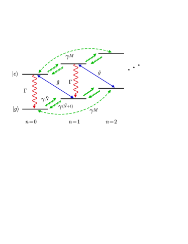
Figure 4: Coherent and incoherent processes in the squeezed frame as described by master equation (18). In this picture the qubit is only excited on the red sideband ($\tilde{g}$). Followed by a spontaneous decay ($\Gamma$) these transitions cool the oscillator to its ground state. The cooling is compensated by the squeezed heat bath which apart from the enhanced heating rate ($\gamma\tilde{N}$) also induces coherences between the states $|n\rangle$ and $|n\pm 2\rangle$ ($\gamma M$).

Weak coupling. We first consider the limit where the decay of the charge qubit is much faster than the rest of the system dynamics, $\Gamma\gg\tilde{g}(r),\gamma\tilde{N}(r)$. In this regime the excited state can be adiabatically eliminated by treating the coupling term, $\mathcal{L}_{g}$ in second order perturbation theory. After tracing over the qubit degrees we obtain a new master equation for the oscillator density operator, $\tilde{\rho}_{x}$. The excitations of the charge qubit on the red sideband provide an additional cooling rate of $4\tilde{g}^{2}/\Gamma$ for the resonator. The master equation for the oscillator alone can be solved by transforming it into a partial differential equation for the Wigner function. The details of this calculations are given in Appendix A. In this limit we obtain the result

$$\mathcal{R}=\sqrt{\frac{\frac{2\tilde{g}^{2}}{\Gamma}\,e^{-2r}+\frac{\gamma}{2}(2N_{B}+1)}{\frac{2\tilde{g}^{2}}{\Gamma}+\frac{\gamma}{2}}}\,.$$ (20)

For small r and $\gamma$ this is close to the ideal behavior $\mathcal{R}=e^{-r}$ while for high values of r it saturates at the value of $\mathcal{R}=\sqrt{(2N_{B}+1)}$ which corresponds to the unperturbed thermal state.

Strong coupling. In the strongly driven regime, $\tilde{g}\gg\Gamma,\gamma\tilde{N}$, the system performs rapid oscillations between the states $|n,g\rangle$ and $|n-1,e\rangle$ on a timescale which is much faster than the incoherent processes. It is therefore convenient to work in the basis of dressed states $|\tilde{n},\pm\rangle=\frac{1}{\sqrt{2}}(|n,0\rangle\pm|n-1,1\rangle)$, $|\tilde{0}\rangle=|0,0\rangle$. Since these are the eigenstates of the Hamiltonian $H=\tilde{g}(a\sigma_{+}+a^{\dagger}\sigma_{-})$ the steady state density operator of Eq. (18) becomes diagonal in that basis as $\tilde{g}\rightarrow\infty$. By neglecting the off-diagonal terms the density operator can be approximated as

$$\tilde{\rho}=p_{0}|\tilde{0}\rangle\langle\tilde{0}|+\sum\,p_{n}^{+}|\tilde{n},+\rangle\langle\tilde{n},+|+p_{n}^{-}|\tilde{n},-\rangle\langle\tilde{n},-|.$$ (21)

Because the Liouville operators $\mathcal{L}_{\Gamma}$ and $\mathcal{L}_{\gamma}$ do not discriminate between the states $|\tilde{n},\pm\rangle$ we define the joint probabilities $p_{n}=p_{n}^{+}+p_{n}^{-}$. With this ansatz the master equation (18) reduces to the rate equation

$$\begin{split}\dot{p}_{n}=&+T_{+}(n-1)p_{n-1}+T_{-}(n+1)p_{n+1}\\ &-\left[T_{+}(n)+T_{-}(n)\right]p_{n}\,,\end{split}$$ (22)

with the heating and cooling rates

$$\begin{split}T_{-}(n)&=(\Gamma+\gamma(\tilde{N}+1)(2n-1))/2,\qquad T_{-}(0)=0\,,\\ T_{+}(n)&=\gamma\tilde{N}(2n+1)/2,\qquad T_{+}(0)=\gamma\tilde{N}\,.\\ \end{split}$$ (23)

In the stationary state the occupation numbers are determined by the detailed balance condition $T_{-}(n+1)p_{n+1}=T_{+}(n)p_{n}$ and an analytic expression for the mean occupation number is given by

$$\langle a^{\dagger}a\rangle_{\tilde{\rho}}=\frac{\gamma\tilde{N}\left(2\,_{2}F_{1}[\frac{3}{2},2,\frac{3}{2}+\alpha,z]-\,_{2}F_{1}[1,\frac{3}{2},\frac{3}{2}+\alpha,z]\right)}{\Gamma+\gamma(\tilde{N}+1)+\gamma\tilde{N}\,_{2}F_{1}[1,\frac{3}{2},\frac{3}{2}+\alpha,z]}\,.$$ (24)

${}_{2}F_{1}$ denotes the hypergeometric function depending on the parameter $\alpha=\Gamma/(2\gamma(\tilde{N}+1))$ and is evaluated at the argument $z=\tilde{N}/(\tilde{N}+1)$. Since $\langle a^{2}\rangle_{\tilde{\rho}}$, $\langle a^{{\dagger}2}\rangle_{\tilde{\rho}}\rightarrow 0$ in the limit of strong coupling, a transformation back to the original frame simply gives

$$\mathcal{R}=e^{-r}\sqrt{2\langle a^{\dagger}a\rangle_{\tilde{\rho}}+1}.$$ (25)

Perturbation theory. The interesting regime where the final state of the resonator is squeezed, $\mathcal{R}<1$, obviously requires $\gamma\tilde{N}\ll\tilde{g},\Gamma$. With this restriction a solution for arbitrary parameters $\tilde{g}$ and $\Gamma$ can be found by taking the ideal solution, $\tilde{\rho}=|0,g\rangle\langle 0,g|$ and treat the corrections of $\mathcal{L}_{\gamma}$ in first order perturbation theory. The details of the calculations are listed in Appendix B and the result of this approach is

$$\mathcal{R}=\,e^{-r}\sqrt{1+\frac{\gamma\Gamma|M|}{2\tilde{g}^{2}}+\gamma\tilde{N}\left(\frac{2}{\Gamma}+\frac{\Gamma}{2\tilde{g}^{2}}\right)}\,.$$ (26)

While this expression gives the correct interpolation between the weak and the strong coupling limit it is only valid for $\langle a^{\dagger}a\rangle_{\tilde{\rho}}\ll 1$. A rough estimation shows that this is still true up to the minimum, $\mathcal{R}_{\rm min}\!=\!{\rm min}\{\mathcal{R}(r),r>0\}$ in the case of $g_{1}<\Gamma$ while expression (26) gives rather poor results for $\mathcal{R}_{\rm min}$ in the case of $g_{1}>\Gamma$.

Numerical results. For numerical calculations the master equation (18) is evaluated in the number basis. In the squeezed frame the solution is close to the ground state so a relatively small number of matrix elements is sufficient to describe the exact state. Fig. 5 shows numerically calculated values of $\mathcal{R}_{\rm min}$ for various parameter values for $g_{1}$, $\Gamma$ and $\gamma$. The results show that the noise, $\Delta X_{1}$ can be reduced to half of the standard quantum limit for damping rates $\gamma\geq 0.02$. This corresponds to a Q-factor of 5000 in the case of a 100 MHz resonator. For $Q=10^{5}$ a reduction by a factor of 5 is possible, still assuming a “hot” environment of about $T\approx 20-30$ mK. Obviously, higher oscillator frequencies or lower temperatures would improve the results even further.

Figure 5: Minimum values for the noise reduction, $\mathcal{R}_{\rm min}$ for various parameter values, $g_{1}$, $\Gamma$, $\gamma$ (all in MHz) and $N_{B}=5$. Figure a) shows the dependence of $\mathcal{R}_{\rm min}$ on the driving strength, $g_{1}$ for a fixed $\Gamma=2$, while b) shows the dependence on the decay rate of the charge qubit, $\Gamma$ for fixed $g_{2}=5$. The different values for $\gamma$ in a) and b) are 0.001 (solid), 0.005 (dashed), 0.01 (dotted) 0.02 (dashed-dotted). In Figure c) $\mathcal{R}_{\rm min}$ is plotted as a function of the phonon damping rate, $\gamma$ for $g_{1}=5$ and $\Gamma=2$ (solid), $\Gamma=5$ (dashed), $\Gamma=8$ (dotted).

V Detection of a squeezed state

Below we discuss schemes for detecting non-classical states, in particular squeezed states, of a nanomechanical system. The displacement measurements based on laser interferometry, which are used for mechanical resonators with a length in the order of a hundred microns, cannot be applied in the nanometer regime. Alternatively displacement detectors based on a single electron transistor (SET) Devoret and Schoelkopf (2000) have been considered Blencowe and Wybourne (2000b); Mozyrsky et al. (2004) and were recently used by the groups of A. Cleland Knobel and Cleland (2003) and K. Schwab LaHaye et al. (2004) to measure the fluctuation spectrum of nanomechanical resonators. While in current experiments the displacement sensitivity is still limited by the amplifier noise, the quantum limit is determined by the back action of the current shot noise on the resonator. By increasing the signal amplification of the detector, which is necessary to observe the reduced fluctuations of a squeezed state also this back action is enhanced. A quantum mechanical analysis of the properties of SET-based displacement detectors is presented in Mozyrsky et al. (2004); Clerk and Girvin (2004). Using the results of the analysis done by Mozyrski et al. Mozyrsky et al. (2004) the charge fluctuations on the SET island would destroy the squeezed state, especially in the experimentally attractive sequential tunneling regime.

In quantum optics with trapped ions and in Cavity QED experiments, information about the oscillator state is often obtained via a coupling to a two level atom. Efficient readout techniques for the state of an atom can be used to measure properties of the not easily accessible oscillator mode. Since CPB and other TLS are currently developed for quantum computation  Yu. Makhlin et al. (2001); Vion et al. (2002); Astafiev et al. (2004), which in particular implies a read out of the qubit represented by e.g. the charge states of the CPB, this “measurement toolbox” is being developed in mesoscopic physics. Motivated by this, we discuss the detection of the resonator state via the readout of the charge qubit. We concentrate on two detection methods that can be performed with the setup shown in Fig. 3 extended by a measuring device for the state of the CPB.

V.1 Dark Resonance

A simple way to verify the generation of a squeezed oscillator state is to look at the excited state population, $p_{e}$ of the charge qubit. Since the squeezed state is a dark state of the system Hamiltonian (13) the qubit excitations are significantly suppressed even in the presence of the driving fields. By varying the detuning $\delta_{x}$ a dark resonance becomes visible at $\delta_{x}=0$ Cirac et al. (1993) which corresponds to the generation of a squeezed state. Fig. 6 shows the expected correlations between the degree of squeezing and the steady state excitations of the qubit as a function of the detuning $\delta_{x}$.

In the presence of a finite $\gamma$ the population $p_{e}$ retains at a value of about $\gamma\tilde{N}/\Gamma\ll 1$ (see Appendix B). In the regime of strong coupling, $g_{1},g_{2}\gg\Gamma$ this is clearly distinguishable from the value $p_{e}\approx 1/2$ as expected for, e.g. a thermal state. For weak driving fields and a thermal oscillator state we expect a excited state population of $p_{e}\approx\langle\hat{n}\rangle g_{1}^{2}/\Gamma^{2}+(\langle\hat{n}\rangle+1)g_{2}^{2}/\Gamma^{2}$. Therefore the condition $g_{2}^{2}/\Gamma>\gamma\tilde{N}$ to distinguish the squeezed state from a low temperature thermal state.

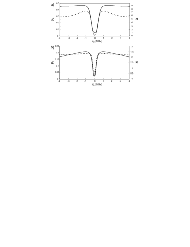
Figure 6: Correspondence between the excited state population, $p_{e}$ (solid line) and the degree of squeezing, $\mathcal{R}$ (dashed line) as a function of the detuning, $\delta_{x}$. The values are plotted for the parameter values $\gamma=0.01$ MHz, $r=0.7$ and $N_{B}=5$ for a) $g_{1}=5$ MHz, $\Gamma=2$ MHz (strong coupling) and b) $g_{1}=1.5$ MHz, $\Gamma=5$ MHz (weak coupling).

V.2 Occupation Numbers

According to its definition (Eq. (1)) a characteristic property of the (ideal) squeezed state, $|\epsilon\rangle$ is that only the even number states are populated. The measurement of the resonator populations via the Stark shift of the qubit resonance frequency was proposed in Ref. Irish and Schwab (2003) while in Ref. Santamore et al. (2003) it is suggested to utilize the anharmonic coupling between bending modes for a Fock state readout. Here we follow a different line Meekhof et al. (1996) and use the linear coupling to the TLS to determine the occupation numbers, $Q_{n}=\langle n|\rho_{x}|n\rangle$. The basic idea is as follows. Suppose we start from an initial density operator $\rho(0)=\rho_{x}\otimes|g\rangle\langle g|$ and switch on a Jaynes-Cummings coupling, $H_{\mathrm{I}}=\hbar g(a\sigma_{+}+a^{{\dagger}}\sigma_{-})$ between the charge qubit and the resonator. The evolution of the qubit polarization is then given by

$$\langle\sigma_{z}\rangle(t)=-\sum_{n}Q_{n}\cos(2\Omega_{n}t)\,.$$ (27)

Due to the different Rabi frequencies $\Omega_{n}=g\sqrt{n}$ the values of $Q_{n}$ can be extracted from the Fourier transform of this signal.

In our system the required coupling of the oscillator to the qubit is realized by Hamiltonian (13) with $g_{1}=g$ and $g_{2}=0$. In contrast to the ideal situation of Eq. (27) the decay of the charge qubit and thermalization of the resonator mode lead to modifications of the signal and restrict the applicability of this method.

Obviously, a necessary condition to resolve the oscillations of the qubit polarization is the strong coupling regime $g\gg\Gamma,\gamma(N_{B}+1)$. An approximate time evolution of the system can be obtained by the following considerations. Starting from a pure state $|n,g\rangle$ the system will oscillate between this state and $|n-1,e\rangle$ with a frequency $2\Omega_{n}$, where $\Omega_{n}=g\sqrt{n}$. During this oscillation it decays into neighboring number states with a rate $R_{n}\equiv T_{+}(n)+T_{-}(n)$ as defined in Eq. (23). Since all other states, $|m\not=n,g\rangle$ and $|m\not=n-1,e\rangle$ are populated gradually their oscillations wash out and with the exception of the ground state they give no contribution for $\sigma_{z}(t)$ . Therefore, for the initial state $|n,g\rangle$ we obtain

$$\langle\sigma_{z}\rangle(t)=-p_{0}(n,t)-\cos(2\Omega_{n}t)\,e^{-R_{n}t}\,,$$ (28)

where $p_{0}(t)$ is the population which accumulates in the ground state which has the form

$$p_{0}(n,t)=1-e^{-\Gamma t/2}\sum_{k=0}^{n-1}\frac{1}{k!}\left(\frac{\Gamma t}{2}\right)^{k}\,,$$ (29)

in the limit $\Gamma\gg\gamma(N_{B}+1)$. The exact time dependence for $\gamma>0$ is not important since the changes of $p_{0}(n,t)$ are slow compared to the Rabi oscillations. For an arbitrary initial state with occupation numbers $Q_{n}$ the polarization of the qubit is given by

$$\langle\sigma_{z}\rangle(t)=-\sum_{n}Q_{n}\left(p_{0}(n,t)+\cos(2\Omega_{n}t)\,e^{-R_{n}t}\right)\,.$$ (30)

The extraction of the occupation probabilities from a given function $\langle\sigma_{z}\rangle(t)$ requires the resolution of the individual Lorentzian peaks in the Fourier transform of this signal. The $n-$th peak can be resolved if the condition $R_{n}+R_{n+1}<g/\sqrt{n}$ is true. Therefore, a lower bound for the maximum occupation probability which we can determine with this method is given by the solution of the equation

$$(\Gamma+2\gamma N_{B})n_{\mathrm{max}}^{1/2}+2\gamma(2N_{B}+1)n_{\mathrm{max}}^{3/2}=g\,.$$ (31)

A first order approximation, valid for $\gamma g^{2}/\Gamma^{2}\ll 1$ gives

$$n_{\mathrm{max}}\simeq\frac{g^{2}}{\Gamma^{2}}\left(1-\frac{4\gamma(2N_{B}+1)g^{2}}{\Gamma^{3}+6\gamma(2N_{B}+1)g^{2}}\right)\,.$$ (32)

For the parameter values $g=5\,\Gamma$, $N_{B}=5$ and $\gamma=0.001\,-\,0.01\,\Gamma$ we obtain $n_{\mathrm{max}}\approx 8-17$, which is sufficient to detect slightly squeezed or low number states.

Fig. 7 shows the time evolution of $\langle\sigma_{z}\rangle(t)$ and the extracted occupation probabilities, $Q_{n}$ for a non-ideal squeezed state. A clear distinction between the squeezed state and a thermal state with the same mean occupation number is possible.

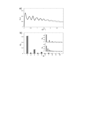
Figure 7: Measurement of the oscillator occupation numbers, $Q_{n}$. A squeezed state is generated as explained in the previous sections with (all in MHz) $g_{1}=5$, $g_{2}=3.5$ ($r\!=\!0.88$), $\Gamma=2$, $\gamma=0.01$ and $N_{B}=5$ MHz. For the detection we assume the same values but $g\!=\!g_{1}\!=\!8$ and $g_{2}=0$. Figure a) shows the exact time evolution of $\langle\sigma_{z}\rangle(t)$ (solid) which is compared to the expected behavior (dashed) as given in Eq. (28). The difference for larger times is due to the deviations of the exact time dependence of $p_{0}(n,t)$ from Eq. (29) for $\gamma>0$. In Figure b) the extracted occupation probabilities (dark gray) are compared with the exact values (light gray). The inset shows the estimated number distribution for a ideal squeezed state (top) and a thermal state with the same mean occupation number, $\langle n\rangle=1$ (bottom).

Although this method provides a complete determination of the number state populations for states close to the ground state, it is not possible to distinguish between coherent superpositions and mixed states. Therefore, in the next section, we discuss the implementation of quantum state tomography to obtain the full information about the resonator’s density matrix.

VI Quantum State Tomography

The ultimate determination of an arbitrary quantum state is the measurement of the complete density operator. The procedure of estimating the density matrix by repeated measurements on the same initial state is called quantum tomography D’Ariano et al. (2003). For a harmonic oscillator the Wigner function of a state, a quasi probability distribution in phase space Gardiner and Zoller (2000); Schleich (2001), contains the same information as the density matrix. The implementation of a method to reconstruct the Wigner function for a nanomechanical resonator provides an universal tool to detect and characterize various non-classical states, and therefore a tool to clearly demonstrate the quantum nature of this still macroscopic system.

In quantum optics methods for state tomography are well known Vogel and Risken (1989); Lutterbach and Davidovich (1997); Schleich (2001) and have been successfully implemented to detect non-classical states of a cavity field See, for example, or the motion of a trapped ion Leibfried et al. (1996). We consider the method discussed in Ref. Leibfried et al. (1996) and show that it is appropriate for the implementation in nano scale mechanical systems.

To determine the Wigner function at a certain point in phase space, $\alpha=x+ip$ we start from the identity Schleich (2001)

$$W(\alpha)=\frac{2}{\pi}\sum_{n=0}^{\infty}(-1)^{n}Q_{n}(\alpha)\,,$$ (33)

where $Q_{n}(\alpha)=\langle n|D^{{\dagger}}(\alpha)\rho_{x}D(\alpha)|n\rangle$ are the occupation probabilities of the displaced density operator. The values of $Q_{n}(\alpha)$ are measured as discussed in the previous section.

A complete state tomography consists of the following steps. For each point in phase space $(x,p)$ we displace the original density operator by $\alpha=-(x+ip)$. Then the occupation numbers of the oscillator are determined by measuring the time evolution of the qubit polarization, $\langle\sigma_{z}\rangle(t)$. In the end we obtain the measured value of the Wigner function, $\tilde{W}(\alpha)$ by summing up the $Q_{n}(\alpha)$ according to Eq. (33).

In the following we discuss the limits for the implementation of the individual steps for a system consisting of a nanomechanical resonator coupled to a charge qubit.

Applying the displacement operator. The first step of the procedure described above requires the shift of the oscillator by the complex amplitude $\alpha$. In the setup shown in Fig. 3 this displacement can be achieved either by applying an additional voltage to a lead opposite the CPB or by exploiting the existing coupling to the charge qubit, $\lambda(t)(a+a^{{\dagger}})\sigma_{x}$.

In the first case a voltage drop $V_{d}$ over a capacitance $C_{d}(x)$ formed by the lead and the resonator generates the driving Hamiltoninan, $H_{d}=\lambda(t)(a+a^{{\dagger}})$ with $\lambda=\frac{1}{2}C_{d}V_{d}^{2}x_{0}/d$. The evolution of the oscillator under $H=\hbar\nu a^{{\dagger}}a+H_{d}$ is Gardiner and Zoller (2000)

$$|\psi(t)\rangle=\hat{D}(\alpha(t))e^{-i\nu ta^{{\dagger}}a}|\psi(0)\rangle\,,$$ (34)

with

$$\alpha(t)=-i\int_{0}^{t}\,dt^{\prime}\,e^{i\nu(t-t^{\prime})}\lambda(t^{\prime})$$ (35)

Because $\lambda\sim 1$ GHz $\gg\nu$, a short constant voltage pulse is sufficient to obtain displacements of $|\alpha|\leq 10$.

If the coupling to the CPB is used for the displacement, we first transfer the ground state of the qubit $|0\rangle$ into one of the eigenstates of $\sigma_{x}$ by adiabatically changing the CPB parameters $V_{g}^{0}$ and $E_{J}$. Since the coupling strength, $\lambda\approx$ 5-10 MHz is much lower than the oscillator frequency a radio frequency pulse $\lambda(t)\sim\cos(\nu t)$ has to be applied to achieve shifts in the order of $|\alpha|\geq 1$.

Especially in the second case the Wigner function of the oscillator is modified during the displacement due to thermalization with the phonon bath. The diffusive dynamics of a driven oscillator and therefore the resulting errors can be calculated exactly (see Appendix C). If we assume an initial Gaussian distribution and a displacement time $\Delta t=|\alpha|/|\lambda|\ll 1/\gamma$ we obtain the relative errors for the widths

$$\varepsilon(\Delta_{x,p}^{2})=\frac{\gamma|\alpha|}{|\lambda|}\left(1+\frac{N_{B}+\frac{1}{2}}{2\Delta_{x,p}^{2}}\right)\,.$$ (36)

The damping also modifies the displacement amplitude. Together with the deviation caused by a small detuning in the driving frequency $\omega=\nu+\delta_{x}$, we obtain a relative error

$$\varepsilon(|\alpha|)=\frac{|\alpha|}{|\lambda|}\left(\frac{|\delta_{x}|}{2}+\frac{\gamma}{4}\right)\,.$$ (37)

For the parameter values considered in this paper $\varepsilon(|\alpha|)\sim 10^{-3}$.

Occupation numbers. The measurement of the probabilities, $Q_{n}(\alpha)$ is done as discussed in the previous section.

For an estimation of the error due to truncation we consider an initially density matrix of a pure number state, $\rho=|m\rangle\langle m|$ with $m<n_{\mathrm{max}}$. The application of the displacement operator shifts some part of the wavefunction out of the detectable subspace $\{|0\rangle,\dots,|n_{\mathrm{max}}\rangle\}$. This leads to an absolute error in the estimated Wigner function $\tilde{W}(\alpha)$ of

$$\varepsilon(m,\alpha)=|\tilde{W}(\alpha)-W(\alpha)|\leq\frac{2}{\pi}\sum_{k=n_{\mathrm{max}}}^{\infty}|\langle k|\hat{D}(-\alpha)|m\rangle|^{2}\,.$$ (38)

The matrix elements of the displacement operator are given by

$$|\langle k|\hat{D}(-\alpha)|m\rangle|^{2}=\frac{m!}{k!}|\alpha|^{2(m-k)}e^{-|\alpha|^{2}}\left[L_{m}^{k-m}(|\alpha|^{2})\right]^{2}\,$$

where $L_{m}^{k-m}$ are the generalized Laguerre polynomials. The sum $\sum_{m}\langle m|\rho|m\rangle\,\varepsilon(m,\alpha)\ll 1$ provides an upper bound for the total truncation error and rough estimation whether the method is applicable or not. In practice the determination of the $Q_{n}$ is done by fitting the actual signal by minimizing the deviations in the least square sense. For a linear fit the standard deviation of the $Q_{n}$ can be written as

$$\sigma(Q_{n})=c_{n}\sigma_{D}\,.$$ (39)

The error in the measured data point, $\sigma_{D}$ includes the error from the measurement of the qubit polarization as well as deviations of the system evolution from expected evolution as given in Eq. (28). The coefficients, $c_{n}$ depend on the parameters of the system and the fitting procedure Press et al. (1992). While the $c_{n}$ increase on a scale set by $n_{\rm max}$ it is still possible to determine the $Q_{n}$ beyond $n_{\rm max}$ in the expense of accuracy. For the example given below the $c_{n}$ are shown in Fig. 8.

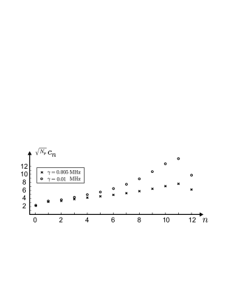
Figure 8: Coefficients, $c_{n}$ which determine the error of the estimated occupation numbers according to Eq. (39). For a large number of measured data points, $N_{D}$ the $c_{n}$ are proportional to $1/\sqrt{N_{D}}$. See text for details.

Example. To summarize the considerations made in this section we discuss the generation of a squeezed state and the reconstruction of its Wigner function for a specific example in some detail. We consider a nanomechanical resonator with a fundamental frequency of $100$ MHz and a $Q$-value of $2\times 10^{4}$ cooled to a temperature of $25$ mK. For the coupling to the CPB we assume the values $g_{1}=5$ MHz, $g_{2}=3$ MHz ($r=0.7$) and a decay rate $\Gamma=2$ MHz. Using the results of the last section, this drives the resonator into a state with a noise reduction $\mathcal{R}\approx 0.5$ in one quadrature components. After the resonator has reached its steady state we switch off the coupling and wait for a short time $\tau\sim 1/\Gamma$ to reduce the excited state population to less than 1%. According to Eq.  (36) this delay leads to a broadening in the $X_{1}$ direction of about 17%, so we end up with $\mathcal{R}\approx$ $0.6$. The exact Wigner function for this state is well located in a the phase space region $|\alpha|\leq 2$.

For the displacement of the oscillator we use the coupling to the CPB as described above with $\lambda=8$ MHz. Eq. (36) predicts an error of $\varepsilon(\Delta_{x}^{2})\approx|\alpha|\times$2%

For the determination of the occupation numbers, $Q_{n}(\alpha)$ we apply a red sideband signal with $g=8$ MHz. For this value we obtain $n_{\mathrm{max}}\approx 8$. The estimation $\sum_{m}\langle m|\rho|m\rangle\,\varepsilon(m,\alpha)\leq 0.15$ for the phase space region $|\alpha|\leq 2$ shows that an accurate reconstruction of the Wigner function is possible. To resolve oscillations of frequency $g\sqrt{n_{\mathrm{max}}}$ over a time much longer than the characteristic decay time the number of measured data point, $N_{D}$ has to fulfill $N_{D}\gg 2g\sqrt{n_{\mathrm{max}}}/(\pi\Gamma)$. In our example we choose a measurement time $T=3$ $\Gamma^{-1}$ and $N_{D}=150$. For these values the coefficients $c_{n}$ in Eq. (39) are plotted in Fig. 8. We suppose that the qubit polarization can be measured with an accuracy of $0.02$ and that the values for $Q_{0\dots 12}$ (we choose $n_{\rm max}=12$) are estimated. Adding the errors of the occupation numbers, the error due to truncation and the error from the displacement we expect an accuracy for the reconstructed Wigner function of $|\tilde{W}(\alpha)-W(\alpha)|\leq 0.05$.

The results of a numerical simulation of the generation of the squeezed state and the reconstruction of its Wigner function is shown in Fig. 9.

In Appendix D we also briefly discuss a different method for a state tomography as proposed by Lutterbach and Davidovich Lutterbach and Davidovich (1997). While this method is experimentally more attractive since it requires less measurements, a stronger coupling and longer decoherence times of the qubit are required for its implementation.

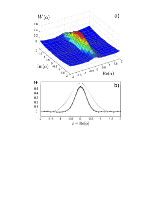
Figure 9: Results of the numerical simulation of the state tomography for a squeezed state as described in Section VI. Figure a) shows the reconstructed Wigner function, $\tilde{W}(\alpha)$. In Figure b) a cut of $\tilde{W}(\alpha)$ (solid line) in x direction (${\rm Im}(\alpha)=0$) is compared with the corresponding values of the real Wigner function, $W(\alpha)$ (dashed line) and the Wigner function of the oscillator ground state (dotted line).

VII Conclusion

In this paper we showed that by reservoir engineering the fundamental mode of a nanomechanical resonator can be driven into a squeezed state. The stationary state exhibits noise reduction in one of the quadrature components by a factor of $\mathcal{R}\approx$ 0.5 - 0.2 below the standard quantum limit. For a 100 MHz resonator these values are obtained for Q-values in the order of $Q=10^{4}-10^{5}$ and standard dilution refrigerator temperatures of T $\approx$ 30 mK. The detection of the squeezed state can be done within the same setup as used for its generation by measuring the excitation probability of the charge qubit. Furthermore this measurement procedure can be extended to obtain a complete reconstruction of the oscillator’s Wigner function. This tool provides an universal detection method for non-classical behavior of the resonator.

Appendix A Adiabatic Elimination

We consider master equation (19) in the limit $\Gamma\gg\tilde{g},\gamma\tilde{N}$. To zero order in $\tilde{g}/\Gamma,\gamma/\Gamma$ the equation reduces to $\partial_{t}\tilde{\rho}=\mathcal{L}_{\Gamma}\tilde{\rho}$ and a steady state solution is located within the subspace $S=\{\tilde{\rho}_{x}\otimes|g\rangle\langle g|\}$. The term $\mathcal{L}_{\gamma}$ leads to a slow dynamic within this subspace while $\mathcal{L}_{g}$ couples S to its complement. Since $\mathcal{L}_{\Gamma}\tilde{\rho}=\mathcal{O}(\Gamma)$, $\forall\rho\notin S$ we can project the master equation (18) on the subspace S and treat the coupling of $\mathcal{L}_{g}$ in perturbation theory. After tracing over the charge qubit states we obtain

$$\frac{d\tilde{\rho}_{x}}{dt}=\mathcal{L}_{\gamma}\tilde{\rho}_{x}-\mathrm{Tr}_{CQ}\{\mathcal{L}_{g}\mathcal{L}_{\Gamma}^{-1}\mathcal{L}_{g}\,\tilde{\rho}_{x}\!\otimes\!|g\rangle\langle g|\}\,.$$ (40)

An evaluation of this expression leads to a master equation for the reduced density operator of the resonator, $\tilde{\rho}_{x}$ given by

$$\begin{split}\frac{d\tilde{\rho}_{x}}{dt}=&\left(\frac{2\tilde{g}^{2}}{\Gamma}+\frac{\gamma}{2}(\tilde{N}+1)\right)\left(2a\tilde{\rho}_{x}a^{\dagger}-a^{\dagger}a\tilde{\rho}_{x}-\tilde{\rho}_{x}a^{\dagger}a\right)\\ &+\frac{\gamma}{2}\tilde{N}\left(2a^{\dagger}\tilde{\rho}_{x}a-aa^{\dagger}\tilde{\rho}_{x}-\tilde{\rho}_{x}aa^{\dagger}\right)\\ &-\frac{\gamma}{2}M\left(2a\tilde{\rho}_{x}a-aa\tilde{\rho}_{x}-\tilde{\rho}_{x}aa\right)\\ &-\frac{\gamma}{2}M^{*}\left(2a^{\dagger}\tilde{\rho}_{x}a^{\dagger}-a^{\dagger}a^{\dagger}\tilde{\rho}_{x}-\tilde{\rho}_{x}a^{\dagger}a^{\dagger}\right)\,.\end{split}$$ (41)

Because the master equation now only contains the operators a and $a^{\dagger}$ it can be transformed into a partial differential equation for the Wigner function Walls and Milburn (1994),

$$\begin{split}\frac{\partial}{\partial t}\tilde{W}(\alpha)=&\left(\frac{2\tilde{g}^{2}}{\Gamma}+\frac{\gamma}{2}\right)\left(\frac{\partial}{\partial\alpha}\alpha+\frac{\partial}{\partial\alpha^{*}}\alpha^{*}\right)\tilde{W}(\alpha)\\ +&\left(\frac{2g^{2}}{\Gamma}+\frac{\gamma}{2}(2\tilde{N}+1)\right)\frac{\partial^{2}}{\partial\alpha\partial\alpha^{*}}\tilde{W}(\alpha)\\ +&\frac{\gamma}{2}\left(M\frac{\partial^{2}}{\partial\alpha^{2}}+M^{*}\frac{\partial^{2}}{\partial\alpha^{*2}}\right)\tilde{W}(\alpha)\,.\end{split}$$ (42)

By introducing the new variables $\tilde{x}$, $\tilde{p}$ defined by $\alpha=(\tilde{x}+i\tilde{p})e^{i\theta/2}$, Eq. (42) separates into two independent Fokker-Planck equations and their steady state solution is

$$\tilde{W}(\tilde{x},\tilde{p})=\mathcal{N}\exp\left(-\left(\frac{2\tilde{g}^{2}}{\Gamma}+\frac{\gamma}{2}\right)\left(\frac{\tilde{x}^{2}}{D_{x}}+\frac{\tilde{p}^{2}}{D_{p}}\right)\right)\,,$$ (43)

where $\mathcal{N}$ is a normalization constant and

$$D_{x,p}=\frac{\tilde{g}^{2}}{\Gamma}+\frac{\gamma}{2}\left(N_{B}+\frac{1}{2}\right)e^{\pm 2r}\,.$$

Because these calculations have been performed in the squeezed frame we need another change of variables to undo this transformation and finally obtain the Wigner function in the original frame,

$$W(x,p)=\mathcal{N}\exp\left(-\frac{1}{2}(x,p)\Sigma^{-1}(x,p)^{T}\right)\,,$$ (44)

where the variance matrix $\Sigma$ is

$$\Sigma^{-1}=\mathbf{T}^{T}\left(\begin{array}[]{cc}k/D_{x}&0\\ 0&k/D_{p}\end{array}\right)\mathbf{T}\,,$$ (45)

with

$$\mathbf{T}\!=\!\left(\begin{array}[]{cc}e^{r}&0\\ 0&e^{-r}\end{array}\right)\left(\begin{array}[]{cc}\cos(\theta/2)&\sin(\theta/2)\\ -\sin(\theta/2)&\cos(\theta/2)\end{array}\right)\,.$$

The variances of the two quadrature components, $X_{1,2}$ are given by the widths of the Gaussian function $W(X_{1},X_{2})$,

$$\begin{split}(\Delta X_{1})^{2}=&\frac{1}{4}\left(\frac{2g^{2}}{\Gamma}\,e^{-2r}+\frac{\gamma}{2}(2N_{B}+1)\right)/\left(\frac{2g^{2}}{\Gamma}+\frac{\gamma}{2}\right)\,,\\ (\Delta X_{2})^{2}=&\frac{1}{4}\left(\frac{2g^{2}}{\Gamma}\,e^{2r}+\frac{\gamma}{2}(2N_{B}+1)\right)/\left(\frac{2g^{2}}{\Gamma}+\frac{\gamma}{2}\right)\,.\end{split}$$ (46)

Appendix B Perturbative Solution

For a weak coupling of the oscillator to the phonon bath we write the master equation (18) as

$$\frac{d\tilde{\rho}}{dt}=\mathcal{L}_{0}(\tilde{\rho})+\mathcal{L}_{\gamma}(\tilde{\rho})$$ (47)

where $\mathcal{L}_{0}=\mathcal{L}_{g}+\mathcal{L}_{\Gamma}$ contains the terms proportional to $\tilde{g}$ and $\Gamma$ with the steady state solution $\tilde{\rho}_{0}=|0\rangle\langle 0|\otimes|g\rangle\langle g|$. In the limit of weak dissipation, $\gamma(\tilde{N}+1)\ll\tilde{g},\Gamma$ we write the density operator as $\tilde{\rho}=\tilde{\rho}_{0}+\tilde{\rho}_{1}$, and calculate the corrections, $\tilde{\rho}_{1}$ up to first order in $\gamma$.

$$\begin{split}\frac{d\tilde{\rho}_{1}}{dt}=&\,\mathcal{L}_{0}(\tilde{\rho}_{1})+\mathcal{L}_{\gamma}(\tilde{\rho}_{0})\\ =&-i[\,\tilde{g}(a\sigma_{+}+a^{\dagger}\sigma_{-})-i\frac{\Gamma}{2}|e\rangle\langle e|,\tilde{\rho}_{1}\,]+\Gamma\sigma_{-}\tilde{\rho}_{1}\sigma_{+}\\ &+\gamma\tilde{N}(|1\rangle\langle 1|\!-\!|0\rangle\langle 0|)+\gamma M|0\rangle\langle 2|+\gamma M^{*}|2\rangle\langle 0|\,.\end{split}$$ (48)

The steady state solution can be calculated e.g. by evaluating this equation in the number state basis. Using the notation $P_{n}=\langle g,n+1|\tilde{\rho}_{1}|e,n\rangle-\langle e,n|\tilde{\rho}_{1}|g,n+1\rangle$, $E_{n}=\langle e,n|\tilde{\rho}_{1}|e,n\rangle$ and $G_{n}=\langle g,n|\tilde{\rho}_{1}|g,n\rangle$, we obtain the set of coupled equations

$$-i\tilde{g}\sqrt{n+1}P_{n}-\Gamma E_{n} = 0\,,$$

$$-\Gamma/2P_{n}-i2\tilde{g}\sqrt{n+1}(E_{n}-G_{n+1}) = 0\,,$$

$$i\tilde{g}\sqrt{n}P_{n-1}+\Gamma E_{n}+\gamma\tilde{N}\delta_{n,1}-\gamma\tilde{N}\delta_{n,0} = 0\,.$$

Because all matrix elements for $n>1$ are zero we find a very simple solution for the mean occupation number and the excited state population

$$\begin{split}\langle\hat{n}\rangle_{\tilde{\rho}}=G_{1}+E_{1}&=\gamma\tilde{N}\left(\frac{1}{\Gamma}+\frac{\Gamma}{4\tilde{g}^{2}}\right)\,,\\ \langle|e\rangle\langle e|\rangle_{\tilde{\rho}}&=E_{0}=\frac{\gamma\tilde{N}}{\Gamma}\,.\\ \end{split}$$ (49)

Another set of equations for the matrix elements between the states $\langle n|$ and $|n+2\rangle$ gives two non-zero contributions for $\langle g,0|\rho_{1}|g,2\rangle$ and $\langle g,2|\rho_{1}|g,0\rangle$ which lead to

$$\langle a^{2}\rangle_{\tilde{\rho}}+\langle a^{{\dagger}2}\rangle_{\tilde{\rho}}=\frac{\gamma\Gamma}{4\tilde{g}^{2}}(M+M^{*})\,.$$ (50)

The variance of the $X_{1}$ quadrature component in the original frame is just given by

$$(\Delta X_{1})^{2}=\frac{e^{-2r}}{4}\left(\langle a^{2}\rangle_{\tilde{\rho}}+\langle a^{{\dagger}2}\rangle_{\tilde{\rho}}+2\langle\hat{n}\rangle_{\tilde{\rho}}+1\right)\,.$$ (51)

This leads to the result of Eq. (26).

Appendix C Dissipative, driven Oscillator

We consider a harmonic oscillator, $H=\hbar\nu a^{{\dagger}}a$ driven by the linear term $H_{d}=\lambda e^{i\nu t}a+\lambda^{\ast}e^{-i\nu t}a^{{\dagger}}$ which is weakly coupled to a reservoir. The master equation in the interaction picture is given by

$$\begin{split}\frac{d\rho}{dt}=-i[\lambda a+\lambda a^{{\dagger}},\rho]&+\frac{\gamma(N_{\mathrm{B}}\!+\!1)}{2}\left(2a\rho a^{{\dagger}}\!-\!a^{{\dagger}}a\rho\!-\!\rho a^{{\dagger}}a\right)\\ &+\frac{\gamma N_{\mathrm{B}}}{2}\left(2a^{{\dagger}}\rho a\!-\!aa^{{\dagger}}\rho\!-\!\rho aa^{{\dagger}}\right)\,.\end{split}$$ (52)

This equation can be transformed into a Fokker-Planck equation for the Wigner function Walls and Milburn (1994). For the coordinates $x=(\alpha+\alpha^{\ast})/2$ and $p=(\alpha-\alpha^{\ast})/2i$ we obtain

$$\begin{split}\frac{dW}{dt}&=\left[\mathrm{Re}(\lambda)\frac{\partial}{\partial p}+\mathrm{Im}(\lambda)\frac{\partial}{\partial x}\right]W\\ &+\frac{\gamma}{2}\left[\left(\frac{\partial}{\partial x}x+\frac{\partial}{\partial p}p\right)+\frac{N_{B}+\frac{1}{2}}{2}\left(\frac{\partial^{2}}{\partial x^{2}}+\frac{\partial^{2}}{\partial p^{2}}\right)\right]W.\end{split}$$ (53)

A general solution for an initial distribution, $W_{i}(\alpha)$ is given by

$$W(\alpha,t)\!=\!\frac{1}{{2\pi\sigma^{2}(t)}}\int\!d^{2}\alpha_{0}\,W_{i}(\alpha_{0})\,\mathrm{exp}\left(\!-\frac{|\alpha-\alpha_{0}e^{-\frac{\gamma t}{2}}|^{2}}{2\sigma^{2}(t)}\right)$$ (54)

with $2\sigma^{2}(t)=(N_{B}+\frac{1}{2})(1-e^{-\gamma t})$. For the special case where the the initial distribution is a Gaussian function centered at the origin the time dependent solution can be evaluated as

$$W(x,p,t)=\mathcal{N}(t)\,\mathrm{exp}\left(-\frac{(x-c_{x}(t))^{2}}{2\Delta x^{2}(t)}-\frac{(p-c_{p}(t))^{2}}{2\Delta p^{2}(t)}\right)\,,$$ (55)

with a normalization factor, $\mathcal{N}(t)$ and the time dependent parameters

$$\begin{split}\Delta x^{2}(t)&=\Delta x^{2}(0)e^{-\gamma t}+\frac{2N_{B}+1}{4}(1-e^{-\gamma t})\,,\\ \Delta p^{2}(t)&=\Delta p^{2}(0)e^{-\gamma t}+\frac{2N_{B}+1}{4}(1-e^{-\gamma t})\,,\\ c_{x}(t)&=2\,\mathrm{Im}(\lambda)(1-e^{-\gamma t/2})/\gamma\,,\\ c_{p}(t)&=2\,\mathrm{Re}(\lambda)(1-e^{-\gamma t/2})/\gamma\,.\end{split}$$ (56)

Appendix D Fast Tomography

The reconstruction of the Wigner function as described in Section VI requires a lot of measurements since it relies on the whole time evolution of the qubit polarization. A direct measurement of the Winger function form a single value of $\langle\sigma_{z}\rangle$ has been proposed by Lutterbach and Davidovich Lutterbach and Davidovich (1997) for Cavity QED and ion traps. Here we give a brief summary of this procedure which relies on the identity

$$W(\alpha)=\frac{2}{\pi}\mathrm{{Tr}\{\hat{D}^{{\dagger}}(\alpha)\rho_{x}\hat{D}(\alpha)e^{i\pi a^{{\dagger}}a}\}\,.}$$ (57)

Again the measurements on the qubit are used to deduce the expectation value of the parity operator, $e^{i\pi a^{{\dagger}}a}$ . To do so we assume that a certain evolution $U$ can be applied to the system with the following properties:

$$U(|g\rangle|n\rangle) = |g\rangle|n\rangle\qquad\mathrm{{if\,\,n\,\,is\,\,odd}\,,}$$

$$U(|g\rangle|n\rangle) = |e\rangle|n\rangle\qquad\mathrm{{if\,\,n\,\,is\,\,even}\,.}$$ (58)

Starting from an initial density operator $\rho(0)=\rho_{x}\otimes|0\rangle\langle 0|$ the Wigner function at the point $\alpha$ can then be reconstructed in three steps: First, apply the displacement operator, $D(-\alpha)=D^{{\dagger}}(\alpha)$. Second, let the system evolve according to Eq. (D) and third, measure the polarization of the charge qubit. Then

$$\langle\sigma_{z}\rangle = \mathrm{{Tr}_{x+CQ}\{U\,D^{{\dagger}}(\alpha)\rho(0)D(\alpha)U^{{\dagger}}\sigma_{z}\}}$$

$$= \mathrm{{Tr}_{x+CQ}\{D^{{\dagger}}(\alpha)\rho(0)D(\alpha)U^{{\dagger}}\sigma_{z}U\}}$$

$$= \mathrm{{Tr_{x}}\{D^{{\dagger}}(\alpha)\rho_{x}D(\alpha)e^{i\pi a^{{\dagger}}a}\}=\frac{\pi}{2}W(\alpha)\,.}$$

Due to the special properties of the evolution operator $U$, the summation of Eq. (33) is performed by the system itself and therefore only one value of $\langle\sigma_{z}\rangle$ already determines $W(\alpha)$.

The crucial point for the implementation of this method in mesoscopic systems is the construction of the time evolution $U$ as given in Eq. (D). It can be achieved with a Hamiltonian of the form Lutterbach and Davidovich (1997)

$$H=\frac{1}{2}(E_{J}+\hbar\Delta(t)a^{\dagger}a)\sigma_{z}+\hbar\nu a^{\dagger}a.$$ (59)

Then a Ramsey interferometry produces the result of Eq. (D) if the waiting time, $\tau$ satisfies $\Delta\tau=\pi$. In Ref. Irish and Schwab (2003) it has been pointed out that a static coupling between the resonator and the CPB leads to the desired shift of the energy splitting of the charge qubit,

$$E_{e,n}-E_{g,n}=E_{J}-2|\lambda|^{2}\frac{(2n+1)E_{J}}{E_{J}^{2}-(\hbar\nu)^{2}}\,.$$ (60)

The number state dependent part of the energy difference, $n\Delta=n\,4|\lambda|^{2}E_{J}/(E_{J}^{2}-(\hbar\nu)^{2})$, can therefore be used to implement $U$. For the parameter values given in the previous parts of this paper ($\lambda\approx 10$ MHz, $\nu\approx 100$ MHz, $E_{J}\approx 10$ GHz) the shift $\Delta=40$ kHz is actually too small but by optimizing the system parameters values for $\Delta$ up to $4$ MHz Irish and Schwab (2003) are possible. With such a system the evolution, U can be performed within the decoherence time, $T_{2}$ of the charge qubit Vion et al. (2002) which would allow the implementation of this fast tomography method.

References

- Cleland (2003) A. Cleland, Foundations of Nanomechanics (Springer, Berlin, 2003).
- Cleland and Roukes (1996) A. N. Cleland and M. L. Roukes, Appl. Phys. Lett. 69, 2653 (1996).
- Huang et al. (2003) X. M. H. Huang, C. A. Zorman, M. Mehregany, and M. L. Roukes, Nature 421, 496 (2003).
- Carr et al. (2001) S. M. Carr, W. E. Lawrence, and M. N. Wybourne, Phys. Rev. B 64, 220101 (2001).
- Blencowe and Wybourne (2000a) M. P. Blencowe and M. N. Wybourne, Physica B 280 (2000a).
- Armour et al. (2002) A. D. Armour, M. P. Blencowe, and K. C. Schwab, Phys. Rev. Lett. 88, 148301 (2002).
- Irish and Schwab (2003) E. K. Irish and K. Schwab, Phys. Rev. B 68, 155311 (2003).
- Eisert et al. (2003) J. Eisert, M. B. Plenio, S. Bose, and J. Hartley, e-print quant-ph/0311113 (2003).
- Braginsky and Khalili (1992) V. B. Braginsky and F. Khalili, Quantum Measurement (Cambridge Univ. Pr., 1992).
- Sidles et al. (1995) J. A. Sidles, J. L. Garbini, K. J. Bruland, D. Rugar, O. Züger, S. Hoen, and C. S. Yannoni, Rev. Mod. Phys. 67, 249 (1995).
- Hopkins et al. (2003) A. Hopkins, K. Jacobs, S. Habib, and K. Schwab, Phys. Rev. B 68, 235328 (2003).
- Wilson-Rae et al. (2004) I. Wilson-Rae, P. Zoller, and A. Imamoglu, Phys. Rev. Lett. 92, 075507 (2004).
- Martin et al. (2004) I. Martin, A. Shnirman, L. Tian, and P. Zoller, Phys. Rev. B 69, 125339 (2004).
- Caves et al. (1980) C. M. Caves, K. S. Thorne, R. W. P. Drever, V. Sandberg, and M. Zimmermann, Rev. Mod. Phys. 52, 341 (1980).
- Walls and Milburn (1994) D. F. Walls and G. J. Milburn, Quantum optics (Springer, Berlin, 1994).
- (16) For reviews on squeezed light see, for example, the special issues J. Mod. Opt. 34 6 (1987); J. Opt. Soc. Am. B 4, 10 (19987) or H. J. Kimble, Phys. Rep. 219, 227 (1992).
- Cirac et al. (1993) J. I. Cirac, A. S. Parkins, R. Blatt, and P. Zoller, Phys. Rev. Lett. 70, 556 (1993).
- Poyatos et al. (1996) J. F. Poyatos, J. I. Cirac, and P. Zoller, Phys. Rev. Lett. 77, 4728 (1996).
- Myatt et al. (2000) C. J. Myatt, B. E. King, Q. A. Turchette, C. A. Sackett, D. Kielpinski, W. Itano, C. Monroe, and D. Wineland, Nature 403, 269 (2000).
- Leibfried et al. (2003) D. Leibfried, R. Blatt, C. Monroe, and D. Wineland, Rev. Mod. Phys. 75, 281 (2003).
- Yu. Makhlin et al. (2001) Yu. Makhlin, G. Schön, and A. Shnirman, Rev. Mod. Phys. 73, 357 (2001).
- Vion et al. (2002) D. Vion, A. Aassime, A. Cottet, P. Joyez, H. Pothier, C. Urbina, D. Esteve, and M. H. Devoret, Science 296, 886 (2002).
- Nakamura et al. (1999) Y. Nakamura, Yu. A. Pashkin, and J. S. Tsai, Nature 398, 786 (1999).
- Gardiner and Zoller (2000) C. W. Gardiner and P. Zoller, Quantum Noise (Springer, Berlin, 2000).
- Devoret and Schoelkopf (2000) M. H. Devoret and R. J. Schoelkopf, Nature 406, 1039 (2000).
- Mozyrsky et al. (2004) D. Mozyrsky, I. Martin, and M. B. Hastings, Phys. Rev. Lett. 92, 018303 (2004).
- Blencowe and Wybourne (2000b) M. P. Blencowe and M. N. Wybourne, Appl. Phys. Lett. 77, 3845 (2000b).
- Knobel and Cleland (2003) R. G. Knobel and A. N. Cleland, Nature 424, 291 (2003).
- LaHaye et al. (2004) M. D. LaHaye, O. Buu, B. Camarota, and K. C. Schwab, Science 304, 74 (2004).
- Clerk and Girvin (2004) A. A. Clerk and S. M. Girvin, cond-mat/0405687 (2004).
- Astafiev et al. (2004) O. Astafiev, Y. A. Pashkin, T. Yamamoto, Y. Nakamura, and J. S. Tsai, Phys. Rev. B 69, 180507 (2004).
- Santamore et al. (2003) D. H. Santamore, A. C. Doherty, and M. C. Cross, e-print cond-mat/0308210 (2003).
- Meekhof et al. (1996) D. M. Meekhof, C. Monroe, B. E. King, W. M. Itano, and D. J. Wineland, Phys. Rev. Lett. 76, 1796 (1996).
- D’Ariano et al. (2003) G. M. D’Ariano, M. G. A. Paris, and M. F. Sacchi, Advances in Imaging and Electron Physics 128, 205 (2003).
- Schleich (2001) W. P. Schleich, Quantum Optics in Phase Space (WILEY-VCH, Berlin, 2001).
- Vogel and Risken (1989) K. Vogel and H. Risken, Phys. Rev. A 40, 2847 (1989), for a review see, for example, the special issue of the journal J. Mod. Opt. 44, 11 (1997).
- Lutterbach and Davidovich (1997) L. G. Lutterbach and L. Davidovich, Phys. Rev. Lett. 78, 2547 (1997).
- (38) See, for example,, G. Breitenbach, S. Schiller, and J. Mlynek, Nature, 387, 471 (1997); P. Bertet, A. Auffeves, P. Maioli, S. Osnaghi, T. Meunier, M.Brune, J. M. Raimond, and S. Haroche, Phys. Rev. Lett. 89, 200402 (2002).
- Leibfried et al. (1996) D. Leibfried, D. M. Meekhof, B. E. King, C. Monroe, W. M. Itano, and D. J. Wineland, Phys. Rev. Lett. 77, 4281 (1996).
- Press et al. (1992) W. H. Press, S. A. Teukolsky, W. T. Vetterling, and B. P. Flannery, Numerical Recipes (Cambridge University Press, Cambridge, 1992).