Bubble Relaxation Dynamics in Double-Stranded DNA

Abstract

The paper deals with the two-state (opening-closing of base pairs) model used to describe the fluctuation dynamics of a single bubble formation. We present an exact solution for the discrete and finite size version of the model that includes end effects and derive analytic expressions of the correlation function, survival probability and lifetimes for the bubble relaxation dynamics. It is shown that the continuous and semi-infinite limit of the model becomes a good approximation to exact result when $a^{N}\ll 1$, where $N$ is bubble size and $a$, the ratio of opening to closing rates of base pairs, is the control parameter of DNA melting.

Upon heating, a double stranded DNA (ds DNA) undergoes a denaturation process with the formation of bubbles of increasing size and number and, eventually, leading to the separation of the two strands PS70 . On the other hand, many of DNA biological activities require the unzipping of the two strands by breaking hydrogen bonds between base pairs. Such open regions of complex DNA, enclosing up to $10-30$ broken base pairs, represent a first step of the transcription processes and are called the transcription bubbles. Several theoretical models have been proposed to describe the phenomenon of bubble formation (for a review see e.g., WB85 ). However, the issue remains unsettled with various, and even contradictory, results reported in the literature. This is indicative of the complexity of the problem which involves number of factors (e.g., base pair sequences, molecular environment, counterions, and so on) that can influence the denaturation process in various ways (see e.g., PB89 ; KM00 ; SS01 ). In addition, as an one or quasi-one dimensional system, the ds DNA is expected to be very sensitive to thermal fluctuations. Therefore, it seems appropriate in a first step to study the fluctuations of local breathing or unzipping of a ds DNA that opens up bubbles of a few tens of base pairs.

The characteristic dynamics of these local denaturation zones (bubbles) in the structure of a ds DNA have been recently probed through fluorescence correlation spectroscopy BK98 ; ALK03 . This is an essential issue not only for physiological processes involving ds DNA but also for providing insights on the general nature of fluctuations in such systems. From a theoretical modeling perspective, however, we have just begun to understand these experimental results. In their recent paper ALK03 , Altan-Bonnet, Libchaber and Krichevsky (ALK) have presented a measurement of the dynamics of a single bubble formation in ds DNA construct. The authors proposed a simple discrete and finite size model for the description of the dynamics of bubbles while they used a continuous and semi-infinite version of the model to fit their experimental data. In this continuous and semi-infinite limit, the survival probability of the bubble reads ALK03 :

$$B_{\infty,c}(t)=\left(1+\frac{x}{2}\right)\,{\rm erfc}\left[\frac{\sqrt{x}}{2}\right]-\left(\frac{x}{\pi}\right)^{1/2}\,{\rm e}^{-x/4}\>,$$ (1)

where $x=t/\tau_{\infty,c}$ and the bubble lifetime is,

$$\tau_{\infty,c}=\frac{(1+a)}{2k_{-}(1-a)^{2}}\>\>;\>\>a=\frac{k_{+}}{k_{-}}={\rm e}^{-\varepsilon/{\rm k_{B}T}}\>,$$ (2)

where $k_{+}$ and $k_{-}$ are the opening and closing rates of base-pair, respectively, $\varepsilon$ the bubble extension energy and ${\rm k_{B}T}$ the thermal energy. In the same spirit, the dynamics of bubble formation have been studied in terms of Fokker-Planck equation HRM03 . In this paper, we go one step forward in providing the exact solution of the generalized ALK model, taking into account both the discreteness of the system and the finite size and including end effects. Our motivation in this investigation is to provide analytic expressions for bubble relaxation function, relaxation time, and lifetime. Such exact solutions may significantly improve data analyzes and be very relevant for any systems with arbitrary $\varepsilon$ and size $N$.

Following ALK, we denote by $b_{n}(t)$ the probability density of bubbles of size $n$ at time $t$ in the system. Assuming that all conformations of the ds DNA can be described as two states (closed or open), the fluctuations dynamics in the number $n$ of open base-pairs in the bubble is described by the master equation,

$$\left\{\begin{array}[]{ccl}\frac{db_{0}}{dt}&=&k_{-}b_{1}-k_{1}b_{0}\\ \frac{db_{1}}{dt}&=&k_{1}b_{0}+k_{-}b_{2}-(k_{+}+k_{-})b_{1}\\ \cdots&&\cdots\\ \frac{db_{n}}{dt}&=&k_{+}b_{n-1}+k_{-}b_{n+1}-(k_{+}+k_{-})b_{n}\\ \cdots&&\cdots\\ \frac{db_{N}}{dt}&=&k_{+}b_{N-1}+k_{2}b_{N+1}-(k_{+}+k_{-})b_{N}\\ \frac{db_{N+1}}{dt}&=&k_{+}b_{N}-k_{2}b_{N+1}\,,\end{array}\right.$$ (10)

where, in addition to the rates $k_{\pm}$ in ALK model ALK03 , we have explicitly introduced the opening and the closing rates $k_{1}$ and $k_{2}$, respectively, for opening the first and closing the last pairs since two ends of the DNA helix are sealed.

Stationary Distribution: When $k_{1}\neq 0$ and $k_{2}\neq 0$, Eq.(10) admits a stationary solution given by,

$$\frac{b_{\rm st}(n)}{b_{\rm st}(0)}=\left\{\begin{array}[]{ccl}k_{1}a^{n-1}/k_{-}&;&1\leq n\leq N\\ k_{1}a^{N}/k_{2}&;&n=N+1\end{array}\right.$$ (13)

where $b_{\rm st}(0)=1/\left[1+(k_{1}Q/k_{-})+(k_{1}a^{N}/k_{2})\right]$ with $Q=(1-a^{N})/(1-a)$. The equilibrium fraction of DNA molecules that are closed, open and with bubbles in the system are given by $b_{\rm st}(0)$, $b_{\rm st}(N)$, and $f_{b}$, respectively, where

$$f_{b}=\sum_{n=1}^{N}b_{\rm st}(n)=\left(\frac{k_{1}Q}{k_{-}}\right)\,b_{\rm st}(0)\>.$$ (14)

The equilibrium constants $K_{1}$ and $K_{2}$ for the concentrations of species in the reactions in Fig. LABEL:fig1 are:

$$K_{1}=\frac{\mbox{[bubble]}}{\mbox{[closed]}}=\frac{k_{1}}{k_{\rm b}}\>\>\mbox{and}\>\>K_{2}=\frac{\mbox{[open]}}{\mbox{[bubble]}}=\frac{k_{\rm f}}{k_{2}}\>.$$ (15)

where the backward $k_{b}$ and forward $k_{f}$ rates are,

$$k_{\rm b}=\frac{k_{\rm f}}{a^{N}}=k_{-}\,\left[\frac{1-a}{1-a^{N}}\right]\>.$$ (16)

When $k_{1}=k_{2}=0$, the concentration of bubbles tends zero and we have $\mbox{[open]}/\mbox{[closed]}=a^{N}$.

Relaxation Function: To study the fluctuations of bubbles, we consider $\Pi(z,t|n_{0})=\sum_{n=0}^{N+1}z^{n}\,b_{n}(t|n_{0})$ (where $b_{n}(t|n_{0})$ is conditional the probability density of finding a DNA molecule with a bubble of size $n$ at time $t$ given that the size was $n_{0}$ at time $t=0$) the characteristic function for the system prepared with the initial condition, $b_{n}(t=0|n_{0})=\delta_{n,n_{0}}$. The Laplace transform [$\widehat{\Pi}(z,s|n_{0})=\int_{0}^{\infty}\!dt\,\Pi(z,t|n_{0})\,{\rm e}^{-st}$] of $\Pi(z,t|n_{0})$ is obtained as,

$$\widehat{\Pi}(z,s|n_{0})=\frac{1}{D(z,s)}\,\times\left\{-z^{n_{0}+1}\right.$$

$$+\left[D(z,0)+k_{1}(1-z)z\right]\,\widehat{b}_{0}(s|n_{0})$$

$$+\left.\left[D(z,0)-k_{2}(1-z)\right]z^{N+1}\,\widehat{b}_{N+1}(s|n_{0})\right\}$$ (17)

where $D(z,s)=k_{+}[z-z_{1}(s)][z-z_{2}(s)]$ and $z_{1,2}(s)=\left[s/k_{-}+1+a\mp\sqrt{(s/k_{-}+1+a)^{2}-4a}\right]/2a$. The functions $\widehat{b}_{0}(s|n_{0})$ and $\widehat{b}_{N+1}(s|n_{0})$, obtained by requiring that the numerator of $\widehat{\Pi}(z,s|n_{0})$ cancels at the roots of $D(z,s)$, are given by,

$$\widehat{b}_{0}(s|n_{0})=\frac{1}{\Delta}\,\left|\begin{array}[]{ccc}z_{1}^{n_{0}}&&\left[sz_{1}-k_{2}(1-z_{1})\right]z_{1}^{N}\\ \\ z_{2}^{n_{0}}&&\left[sz_{2}-k_{2}(1-z_{2})\right]z_{2}^{N}\\ \end{array}\right|$$ (21)

and

$$\widehat{b}_{N+1}(s|n_{0})=\frac{1}{\Delta}\,\left|\begin{array}[]{ccc}s+k_{1}(1-z_{1})&&z_{1}^{n_{0}}\\ \\ s+k_{1}(1-z_{2})&&z_{2}^{n_{0}}\\ \end{array}\right|$$ (25)

with

$$\Delta(s)=\left|\begin{array}[]{ccc}s+k_{1}(1-z_{1})&&\left[sz_{1}-k_{2}(1-z_{1})\right]z_{1}^{N}\\ \\ s+k_{1}(1-z_{2})&&\left[sz_{2}-k_{2}(1-z_{2})\right]z_{2}^{N}\\ \end{array}\right|\>.$$ (29)

To fit with the experimental conditions by ALK, we assume that the system is prepared in the initial conditions $b_{\rm st}(n_{0})/f_{b}$ for $1\leq n_{0}\leq N$ and zero otherwise. The quantity of interest is the correlation function $C_{N}(t)$ that describes fluctuations in the bubble population at equilibrium and is measured by fluorescence correlation spectroscopy method ALK03 ,

$$C_{N}(t) =\sum_{n_{0}=1}^{N}\sum_{n=1}^{N}\frac{\left[b_{n}(t|n_{0})-b_{n}(\infty|n_{0})\right]\,b_{\rm st}(n_{0})}{f_{b}(1-f_{b})}$$ (30)

$$=1-\sum_{n_{0}=1}^{N}\frac{\left[b_{0}(t|n_{0})+b_{N+1}(t|n_{0})\right]\,b_{\rm st}(n_{0})}{f_{b}(1-f_{b})}$$

in which $b_{n}(0|n_{0})=\delta_{n,n_{0}}$, and we have used the conservation of the probability density, $\sum_{n=0}^{N+1}b_{n}(t|n_{0})=1$. Note that $C_{N}(0)=1$ since $b_{n}(\infty|n_{0})=b_{\rm st}(n)$ and $C_{N}(\infty)=0$. Performing the summation in Eq.(30), we find the Laplace transform of $C_{N}(t)$ as,

$$\widehat{C}_{N}(s)=\frac{1}{s}-\left[\frac{k_{-}}{(1-f_{b})Q}\right]\,\times$$

$$\frac{\left[(1-z_{1})F(z_{2})-(1-z_{2})F(z_{1})\right]}{s}\>,$$ (31)

where $F(z)=$
$(1-z^{N})\left[s(1-z^{N+1})+(1-z)(k_{1}+k_{2}z^{N})\right]/[z^{N}\,\Delta]$. From this, the bubble relaxation time is obtained as $\tau_{N}=\widehat{C}(s=0)$. Two limiting cases are considered depending on $k_{1}$ and $k_{2}$.

$\bullet$ $(k_{1}+k_{2})>0$ limit: In this case, the bubble relaxation time is given by,

$$\tau_{N} = \left\{\frac{(1+a^{N+1})}{(1-a)^{2}}\,\left[\frac{k_{1}+k_{2}}{a^{N}k_{1}k_{-}+k_{2}k_{-}+Qk_{1}k_{2}}\right]\right.$$ (32)

$$- \frac{2Na^{N}}{(1-a)(1-a^{N})}\,\left[\frac{k_{1}+k_{2}}{a^{N}k_{1}k_{-}+k_{2}k_{-}+Qk_{1}k_{2}}\right]$$

$$+ \left(\frac{1-a^{N+1}}{1-a}\right)\,\left[\frac{k_{-}}{a^{N}k_{1}k_{-}+k_{2}k_{-}+Qk_{1}k_{2}}\right]$$

$$- \left.\left(\frac{1-a^{N+1}}{1-a}\right)\,\left[\frac{1}{a^{N}k_{1}+k_{2}}\right]\right\}\,{\rm H}(k_{1}+k_{2})\>,$$

where $\rm H$ is Heaviside step function defined as $\rm{H}(z)=0$ for $z<0$ and $\rm{H}(z)=1$ for $z>0$. When either $k_{1}$ or $k_{2}$ tends to zero, $\tau_{N}$ linearly decreases respectively with either $k_{1}$ or $k_{2}$ towards $\tau_{N}(0)$ defined as,

$$k_{-}\tau_{N}(0) = \left[\frac{(1+a^{N+1})(1-a^{N})-2Na^{N}(1-a)}{(1-a)^{2}(1-a^{N})}\right]$$ (35)

$$\times \left\{\begin{array}[]{ccc}1&;&k_{1}=0\>,\>k_{2}>0\\ a^{-N}&;&k_{1}>0\>,\>k_{2}=0\end{array}\right.$$

Note that $\tau_{N}(0)$ is independent of $k_{1}$ and $k_{2}$ because the kinetics in these limits is dominated by the bubbles decay. As $N\rightarrow\infty$, the fluctuations of bubbles become independent of $N$ with the relaxation function,

$$\widehat{C}(s)=\frac{1}{s}-\frac{k_{-}(1-a)(1-z_{1})}{(1-f_{b})s\left[s+k_{1}(1-z_{1})\right]}\>,$$ (36)

and lifetime,

$$\tau_{\infty}=\frac{1}{(1-a)\left[(1-a)k_{-}+k_{1}\right]}\>.$$ (37)

$\bullet$ $k_{1}=k_{2}=0$ limit: In this case, $\widehat{C}_{N}(s)=\widehat{B}_{N}(s)$, where $B_{N}(t)$ is the survival probability of bubbles. Likewise, the bubble lifetime $\tau_{N}=\widehat{B}_{N}(s=0)$ is given by,

$$\tau_{N}=\frac{(1-a^{N})(1-a^{N+2})-N(N+2)(1-a)^{2}a^{N}}{k_{-}(1-a)^{2}(1-a^{N})(1-a^{N+1})}\>.$$ (38)

When $N\rightarrow\infty$, Eq.(31) reduces to $\widehat{B}_{\infty}(s)=(1/s)-k_{-}(1-a)\,[1-z_{1}]/s^{2}$, and,

$$B_{\infty}(t)=1-\frac{x}{1-a}+$$

$$\frac{(1-a)}{2a}\,\int_{0}^{y}\!dz\,\left(\frac{y}{z}-1\right)\,\exp\left[-\frac{(1+a)}{2\sqrt{a}}\,z\right]\,{\rm I}_{1}[z]\>,$$ (39)

where ${\rm I}_{1}[\cdots]$ is the modified Bessel function of order one, $y=2x\sqrt{a}/(1-a)^{2}$ and $x=t/\tau_{\infty}$. It is worth noting that even in the $N\to\infty$ limit the exact solution Eq.(39) for the bubble survival probability is different from Eq.(1) given in ALK03 . The fact is that, depending on the size $N$ and the parameter “$a$”, the discreteness of the system is an ingredient which might be taken into account to capture the correct bubble dynamics. This is illustrated in Fig. 1 where the exact survival probability is compared with its $N\to\infty$ limit and the ALK continuous model. Figure 2 shows the departure in the bubble lifetime to the continuous limit as a function of bubble size. It clearly appears from Figs. 1 and 2 that the continuous limit as done by ALK ALK03 becomes a fairly good approximation to exact result for $a^{N}\ll 1$ (where $a\leq 1$ is the control parameter for the ds DNA melting ALK03 ; HM03 ).

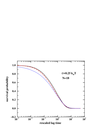
Figure 1: Bubble survival probabilities, from the top to the bottom, $B_{N}(t)$ (solid line), $B_{\infty}(t)$ (long-dashed line) and $B_{\infty,c}(t)$ (dotted line) versus the rescaled lag times $t/\tau_{N}$, $t/\tau_{\infty}$ and $t/\tau_{\infty,c}$, respectively.

Figure 2: Reduced lifetime, $\tau_{N}/\tau_{\infty}$ in Eq.(32) for $k_{1}=0$ (dashed line) and Eq.(38) (solid line), as a function of bubble size, $N$. Quoted numbers represent the bubble extension energy $\varepsilon/{\rm k_{B}T}$.

Simple inspection of expressions in Eqs.(31), (32) and (38), and of the figures, indicate that the behavior of bubble dynamics is controlled by the bubble size $N$ and the parameter $a$ (ratio of opening to closing rates of base-pairs). As $a\leq 1$ according to the experimental situation in ALK03 , the closing of bubbles is the fastest process in the bubbles kinetics. The parameter $a$ also controls the denaturation transition. As $a\to 1$, there is a kind of ”critical slowing down” where the fluctuations of bubbles are described by an unbiased diffusion process. For instance, the bubble lifetime in Eq.(38) reduces to,

$$\tau_{N}=\frac{(N+1)(N+2)}{12k_{-}}\>,$$ (40)

in the $a\to 1$ limit, and $\tau_{N}$ diverges with the bubble size.

It may be useful for practical purposes to have an idea of numerical values of physical parameters entering in the problem. In the absence of direct measurement of $k_{-}$, for instance, one can use the experimental data in ALK03 in conjunction with theoretical results to estimate the closing rate $k_{-}$. The results of such an estimation are presented in Table 1.

Table 1: Estimate of $k_{-}$ using the expressions of the bubble lifetime in the case of $k_{1}=k_{2}=0$. In Ref. ALK03 , the experimental bubble lifetime is equal to $95\,\mu s$ at T=303K for $N=18$ and DNA samples $M_{18}$ and $A_{18}$.

$\varepsilon/{\rm k_{B}T}$		$0.1$		$0.5$		$1$
Lifetime ($\mu s$)		$k_{-}\>\>(\times 10^{6}\,{\rm s}^{-1})$
$\tau_{N}$	$95$	$0.300$		$0.0675$		$0.0263$
$\tau_{\infty}$	$95$	$1.162$		$0.0680$		$0.0263$
$\tau_{\infty,c}$	$95$	$1.110$		$0.0550$		$0.0180$

To summarize, we have presented an exact solution of the discrete and finite size model in Eq.(10) for the description of the fluctuations dynamics of bubble formation. The twofold merit of this two-state (open and closed) model is to already include sufficient complexity of the bubble dynamics over biomolecular relevant scales and to allow exact analytical solution. The mains results of the paper are the expressions in Eqs.(31), (32) and (38) for the bubble correlation function, relaxation time and bubble lifetime, respectively. These results, consistent with available data, may prove to be useful for analysis and interpretation of experimental data on bubble fluctuations and they are amenable for further experimental tests. It is worthwhile to mention in addition that different expressions for the relaxation function and time can be generated within the theoretical framework developed above by simply using different initial conditions in Eq.(30) for the preparation of the system.

Given the closing and opening rates of base pair, the model discussed above allows also to study phenomena related to the denaturation mechanisms of DNA such as heating, changing buffer surrounding, or applying external torques or forces MS95 ; CM99 ; LN00 ; CK02 . Likewise, the model can easily modified to include more than two states in order to describe, for instance, the intermediates states between bond and broken states. Finally, although the calculations may become more involve and intricate, the theory outlined above can be extended in several directions in including in Eq.(10), for example, the effects of base pair sequence in the opening and closing rates (two and three hydrogen bonds being involved in A-T and G-C base pairs, respectively), initiation of several bubbles, bubbles fission and fusion processes, and so on.

References

• (1) D. Poland, H. A. Sheraga, Theory of Helix - Coil Transitions in Biopolymers, Academic Press, New York (1970).
• (2) R. M. Wartell, A. S. Benight, Phys. Rep., 126, 67 (1985).
• (3) M. Peyrard, A. R. Bishop, Phys. Rev. Lett., 62, 2755 (1989).
• (4) Y. Kafri, D. Mukamel, L. Peliti, Phys. Rev. Lett., 85, 4988 (2000).
• (5) N. Singh, Y. Singh, Phys. Rev. E, 64, 042901 (2001).
• (6) G. Bonnet, O. Krichevskii, A. Libchaber, Proc. Natl. Acad. Sci. USA, 95, 8602 (1998).
• (7) G. Altan-Bonnet, A. Libchaber and O. Krichevsky, Phys. Rev. Lett., 90, 138101-1 (2003).
• (8) A. Hanke and R. Metzler, J. Phys. A: Math. Gen. 36, L473 (2003).
• (9) T. Hwa, E. Mariani, K. Sneppen, L-h. Tang, Proc. Natl. Acad. Sci. USA, 100, 4411 (2003).
• (10) J. F. Marko, E. D. Siggia, Phys. Rev. E, 52, 2912 (1995); R. M. Fye, C. J. Benham, Phys. Rev. E. 59, 3408 (1999).
• (11) S. Cocco, R. Monasson, Phys. Rev. Lett., 83, 5178 (1999).
• (12) D. K. Lubensky, D. R. Nelson, Phys. Rev. Lett., 85, 1572 (2000).
• (13) J. Chuang, Y. Kantor, M. Kardar, Phys. Rev. E, 65, 011802 (2002).