Scaling prediction for self-avoiding
polygons revisited

Abstract

We analyse new exact enumeration data for self-avoiding polygons, counted by perimeter and area on the square, triangular and hexagonal lattices. In extending earlier analyses, we focus on the perimeter moments in the vicinity of the bicritical point. We also consider the shape of the critical curve near the bicritical point, which describes the crossover to the branched polymer phase. Our recently conjectured expression for the scaling function of rooted self-avoiding polygons is further supported. For (unrooted) self-avoiding polygons, the analysis reveals the presence of an additional additive term with a new universal amplitude. We conjecture the exact value of this amplitude.

1 Introduction

The model of (planar) self-avoiding polygons [17, 12] is an important unsolved model of statistical physics. Some progress has been made in recent years. Results from exactly solvable polygon models led to a prediction of the scaling function of self-avoiding polygons, counted by perimeter and area [22, 2]. On the other hand, the theory of stochastic processes provided new insight into the problem by relating it to the so-called Schramm-Loewner evolution [16]. In this article, we will further test the predictions implied by the scaling function conjecture [22, 2] and extend it.

Let $p_{m,n}$ denote the number of self-avoiding polygons (SAP) of perimeter $m$ and area $n$ on a given lattice. In this article, we will consider self-avoiding polygons on the square, hexagonal and triangular lattices. Denote the perimeter and area generating function by $G(x,q)=\sum_{m,n}p_{m,n}x^{m}q^{n}$. The function $G(x,1)$ is called the perimeter generating function of the model, its radius of convergence is denoted by $x_{c}$. For SAP, we have for the singular part of the perimeter generating function $G^{(sing)}(x,1)\sim A(1-x/x_{c})^{2-\alpha}$ as $x\to x_{c}$, with $\alpha=1/2$ being universally accepted, though not rigorously proved. (All limits appearing in this paper will be taken from below.) Until section 5, we will concentrate on rooted self-avoiding polygons, whose perimeter and area generating function is $G^{(r)}(x,q)=\sum_{m,n}p^{(r)}_{m,n}x^{m}q^{n}$, where $p^{(r)}_{m,n}=mp_{m,n}$. We thus have $G^{(r)}(x,q)=x\frac{\rm d}{{\rm d}x}G(x,q)$ and $G^{(r),(sing)}(x,1)\sim B(1-x/x_{c})^{1-\alpha}$ as $x\to x_{c}$.

The phase diagram of SAP, enumerated by perimeter and area, appears to have first been discussed in [9]. There is a phase boundary in the region $q<1,$ $x>x_{c},$ terminating in a bicritical point at $(x_{c},1)$. If $q=1$, typical polygons are extended, whereas for $q<1$, typical polygons try to minimise their area. This particular type of phase transition is also called a collapse transition, and the phase $q<1$ is called the branched polymer phase. Indeed, polygons of minimal area may be viewed as branched polymers. The phase boundary is characterised by a logarithmic singularity, when approached from below. This particular feature was first found by studying the area generating function of SAP, $G(1,q)$, which was found (numerically) to have a singularity of the form $G(1,q)\sim A\log(1-q)$ as $q\to 1$ [7]. The point $(x,q)=(x_{c},1)$ is a bicritical point where a generic scaling form of the perimeter and area generating function is expected to hold [9]. The singular behaviour about a bicritical point is generally expected to be of the form

$$G(x,q)\sim G^{(reg)}(x,q)+(1-q)^{\theta}H\left(\frac{x_{c}-x}{(1-q)^{\phi}}\right)\qquad(x,q)\to(x_{c},1),$$ (1.1)

where $G^{(reg)}(x,q)$ denotes the regular part of $G(x,q)$ at $(x,q)=(x_{c},1)$, and $H(s)$ is called the scaling function with critical exponents $\theta$ and $\phi$, and $s=\frac{x_{c}-x}{(1-q)^{\phi}}$. We stress that there are counter-examples known where such a scaling form is not valid, for example, in the simple model of rectangles [13]. For staircase polygons [19], the behaviour (1.1) has been proved. The exponents are $\theta=1/3$, $\phi=2/3$, and the scaling function of staircase polygons is the logarithmic derivative of an Airy function. The phase diagram of staircase polygons is similar to that of SAP. There is also a phase boundary in the region $q<1,$ $x>x_{c}$, terminating in a bicritical point at $(x_{c},1)$. The phase boundary in that case is characterised by a simple pole, when approached from below, while at the bicritical point we have a branch-point singularity $G^{(sing)}(x_{c},q)\sim B(1-q)^{1/3}$ as $q\to 1$, as follows from [19]. Interestingly, rooted SAPs display the same singularity structure as the staircase polygon model. This led to the question whether the scaling functions might be the same [21].

Any conjectured form for the singular behaviour of $G^{(r)}(x,q)$ can most appropriately be tested by comparing predicted moments to those calculated numerically. In [15, 22] we made such a comparison with the area moments, which led us to conjecture the exact form of the scaling function, thereby answering the previous question in the affirmative. We review this calculation below. The validity of the scaling function conjecture leads, in addition, to predictions of the leading singular behaviour of the perimeter moments, as explained in section 3. Checking this behaviour thus yields a further test of the scaling assumption. This was done in [22] only for the moment of order zero, i.e., the (bicritical) area generating function $G^{(r)}(x_{c},q)$ as $q\to 1$. Here we present, for the first time, a detailed numerical analysis for the higher moments, which turns out to be numerically much more difficult than the analysis of the area moments.

After establishing agreement with the predictions of the values of the first 10 perimeter moments in section 4, we consider the scaling functions for (unrooted) SAP, obtained by integration of the rooted SAP scaling function. The “constant” of integration, which must be a function solely of $q$, in order that its derivative with respect to $x$ vanishes, turns out to dominate the behaviour of the scaling function as $q\rightarrow 1.$ We argue for a particular form of this term, and then numerical testing reveals an unexpected amplitude universality across the three lattices we study. Based on our experience with other exact amplitudes, we conjecture the exact value of this universal amplitude. More precisely, we show below that at the bicritical point the behaviour is $G^{(sing)}(x_{c},q)\sim A(1-q)\log(1-q)$ as $q\to 1$, where we conjecture the exact value of the amplitude $A$. Our findings imply that the scaling form (1.1) cannot hold for (unrooted) SAP. We suggest a modified form below, see (5.4), (5.6) and (5.7).

In the last section, we analyse the shape of the critical curve near the bicritical point, which describes the crossover to the branched polymer phase. We find the prediction from the scaling function conjecture satisfied, within numerical accuracy. We also analyse the behaviour of the critical curve as $q\to 0$. Numerical techniques are explained in an appendix.

2 Area moments for rooted SAP

The factorial area moment generating functions $g^{(r)}_{k}(x)$ of rooted self-avoiding polygons are defined by

$$g^{(r)}_{k}(x)=\frac{(-1)^{k}}{k!}\left.\frac{{\rm d}^{k}}{{\rm d}q^{k}}G^{(r)}(x,q)\right|_{q=1}=\frac{(-1)^{k}}{k!}\sum_{m,n}(n)_{k}\,p^{(r)}_{m,n}x^{m},$$ (2.1)

where $(a)_{k}=a(a-1)\cdots(a-k+1)$. Previous numerical analyses [15, 22] based on exact enumeration data provide strong evidence for the asymptotic form

$$g^{(r),(sing)}_{k}(x)\sim\frac{f_{k}}{(x_{c}-x)^{\gamma_{k}}}\qquad(x\to x_{c}),$$ (2.2)

with exponents $\gamma_{k}=(3k-1)/2$. We incorporate the coefficients and exponents into the function $F^{(r)}(s)$ defined by

$$F^{(r)}(s)=\sum_{k=0}^{\infty}\frac{f_{k}}{s^{\gamma_{k}}}.$$ (2.3)

At this stage, the function $F^{(r)}(s)$ should be viewed as some generating function for the numbers $f_{k}$, with $s$ being an undetermined variable. We will argue below that, given the validity of the scaling assumption (1.1), the function $F^{(r)}(s)$ is the scaling function $H^{(r)}(s)$ of the model. (In fact, $F^{(r)}(s)$ is then the generating function of the perimeter moment amplitudes $e_{k}$, which are defined in (3.2)).

In [22], we tested the conjecture that the function $F^{(r)}(s)$ of rooted self-avoiding polygons is given by

$$F^{(r)}(s)=-4f_{1}\frac{d}{ds}\log\mbox{Ai}\left(\left(\frac{f_{0}}{4f_{1}}\right)^{2/3}s\right)$$ (2.4)

by comparing numerical estimates of $f_{k}$ with estimates that follow from (2.4). The constants $f_{0}$ and $f_{1}$ have been numerically determined previously to great accuracy [24]. We have $f_{0}=-\frac{2E_{0}\sqrt{\pi}}{\sigma\sqrt{x_{c}}}$ and $f_{1}=-\frac{E_{1}x_{c}}{\sigma}$, where $x_{c}$ is the radius of convergence of the perimeter generating function, given by $x_{c}=0.379052277757(5)$ on the square lattice, $x_{c}=0.2409175745(3)$ on the triangular lattice, and $x_{c}=1/\sqrt{2+\sqrt{2}}$ on the hexagonal lattice [18]. The constant $\sigma$ is defined such that $p_{m,n}$ is nonzero if $m$ is divisible by $\sigma$. Thus $\sigma=2$ for the square and hexagonal lattices and $\sigma=1$ for the triangular lattice. Estimates of the amplitudes $E_{0}$ and $E_{1}$, taken from [24], are given in Table 1. The value $E_{1}=1/(4\pi)=0.07957747\ldots$ has been derived in [1], using field theoretic arguments.

Amplitude	Square	Hexagonal	Triangular
$E_{0}$	$0.56230130(2)$	$1.27192995(10)$	$0.2639393(2)$
$E_{1}$	$0.0795773(2)$	$0.0795779(5)$	$0.0795765(10)$
$f_{0}$	$-1.61880474(6)$	$-3.0645083(3)$	$-1.906228(1)$
$f_{1}$	$-0.01508198(4)$	$-0.0215332(3)$	$-0.0191714(2)$

Table 1: Values of area moment amplitudes for SAPs taken from [24]

The conjecture (2.4) follows from the assumption that rooted self-avoiding polygons behave asymptotically like models whose perimeter and area generating function are described by a $q$-algebraic functional equation of arbitrary degree with a square-root singularity as the dominant singularity of the perimeter generating function [4, 22, 23]. This class includes a number of exactly solved polygons models such as staircase polygons, column-convex polygons, and bar-graph polygons [20, 12]. For models within this class, the coefficients $f_{k}$ and exponents $\gamma_{k}$ from (2.2) have been explicitly calculated, leading to the expression (2.4). It is interesting to note that the distribution of area in the limit of large perimeter, which can be extracted from (2.4), see also [25, Appendix], is given by the Airy distribution, which appears in a number of related contexts [10, 25].

Assuming the validity of the scaling form (1.1), the singular behaviour of the area moment generating functions (2.2) determines the critical exponents and the scaling function $H^{(r)}(s)$. Taking the limit $q\to 1$ in (1.1), we infer from (2.2), leaving $\gamma_{k}$ unspecified for the moment, that

$$\gamma_{k}=\frac{k-\theta}{\phi}.$$ (2.5)

We also find that the asymptotic expansion of the scaling function $H^{(r)}(s)$ is given by $H^{(r)}(s)=F^{(r)}(s)$, where $F^{(r)}(s)$ is defined in (2.3). Thus, for rooted SAP, the assumption of the scaling form (1.1), together with the result (2.4) for the area moments, leads to exponents $\theta=1/3$ and $\phi=2/3$ and to the scaling function $H^{(r)}(s)=F^{(r)}(s)$, where $F^{(r)}(s)$ is given in (2.4).

3 Perimeter moments

The factorial perimeter moment generating functions $h^{(r)}_{k}(q)$ of rooted self-avoiding polygons at the bicritical point are defined by

$$h^{(r)}_{k}(q)=\frac{(-1)^{k}}{k!}\left.\frac{{\rm d}^{k}}{{\rm d}x^{k}}G^{(r)}(x,q)\right|_{x=x_{c}}=\frac{(-1)^{k}}{k!}\sum_{m,n}(m)_{k}\,p^{(r)}_{m,n}x_{c}^{m}q^{n},$$ (3.1)

The scaling assumption (1.1) leads to a prediction for the behaviour of the perimeter and area generating function in the limit $x\to x_{c}$. The leading singular behaviour of the perimeter moments is given by

$$h^{(r),(sing)}_{k}(q)\sim\frac{e_{k}}{(1-q)^{\beta_{k}}}\qquad(q\to 1),$$ (3.2)

with exponents $\beta_{k}=k\phi-\theta$, where the singular amplitudes $e_{k}$ appear in the expansion of the scaling function $H^{(r)}(s)=F^{(r)}(s)$ about the origin,

$$F^{(r)}(s)=\sum_{k=0}^{\infty}e_{k}s^{k}.$$ (3.3)

We can readily derive formulae for the expansion coefficients $e_{k}$ in (3.3). Note that the scaling function (2.4) satisfies the Riccati equation

$$F^{(r)}(s)^{2}-4f_{1}{F^{(r)}}^{\prime}(s)-f_{0}^{2}=0.$$ (3.4)

Inserting the form (3.3) into (3.4), we obtain for the numbers $e_{n}$ the expression

$$e_{n}=b_{n}f_{1}\left(\frac{f_{0}}{f_{1}}\right)^{(2n+2)/3},$$ (3.5)

where the constants $b_{n}$ are defined by the quadratic recursion

$$4nb_{n}+\delta_{n-1,1}=\sum_{k=0}^{n-1}b_{k}b_{n-1-k}\qquad(n>0).$$ (3.6)

The constants $b_{n}$ are polynomials of degree $n+1$ in $b_{0}$. The value of $b_{0}$, remaining undetermined by (3.4), can be extracted from the limit $s\to 0$ in (2.4) as

$$b_{0}=\frac{3^{\frac{5}{6}}\Gamma(\frac{2}{3})^{2}2^{\frac{2}{3}}}{2\pi}.$$ (3.7)

It is interesting to note that the perimeter moments are related to the area moments of negative order [10, Eqn. (37)]. It follows from (3.5) that the amplitude combinations $e_{k}e_{1}^{-k}e_{0}^{k-1}=b_{k}b_{1}^{-k}b_{0}^{k-1}$ are independent of the amplitudes $f_{0}$ and $f_{1}$. The first few combinations are

$$\begin{split}e_{2}e_{1}^{-2}e_{0}&=1-\frac{4}{27}\frac{\sqrt{3}\pi^{3}}{\Gamma(\frac{2}{3})^{6}},\qquad e_{3}e_{1}^{-3}e_{0}^{2}=1-\frac{8}{81}\frac{\sqrt{3}\pi^{3}}{\Gamma(\frac{2}{3})^{6}},\\ e_{4}e_{1}^{-4}e_{0}^{3}&=1-\frac{10}{81}\frac{\sqrt{3}\pi^{3}}{\Gamma(\frac{2}{3})^{6}},\qquad e_{5}e_{1}^{-5}e_{0}^{4}=1-\frac{4}{27}\frac{\sqrt{3}\pi^{3}}{\Gamma(\frac{2}{3})^{6}}+\frac{16}{1215}\frac{\pi^{6}}{\Gamma(\frac{2}{3})^{12}}.\end{split}$$ (3.8)

In the next section we compare these predictions with the numerical values obtained from our new enumeration data.

4 Perimeter moment analysis

We have generated data for self-avoiding polygons, counted by perimeter and area on the square, hexagonal and triangular lattices, using the finite lattice method. In particular, we determined the numbers $p_{m,n}$ for $n\leq 50$ (square lattice), $n\leq 40$ (hexagonal lattice) and $n\leq 60$ (triangular lattice), for all relevant perimeter lengths. The algorithms used in our SAP enumerations are based on the finite-lattice method devised by Enting [5] in his pioneering work on the enumeration of polygons on the square lattice. Details of the algorithms used to enumerate SAPs on the hexagonal and triangular lattices can be found in [6] and [8], respectively. A major enhancement, resulting in exponentially more efficient algorithms, is described in some detail in [14] while recent work on parallel versions can be found in [15]. All of the algorithms described in these papers are for enumerations by perimeter, but the generalisation to include area is straightforward. The calculations were performed on the server cluster of the Australian Partnership for Advanced Computing (APAC). The calculations for the square lattice required up to 14Gb of memory, and were performed on up to 16 processors using a total of just under 2000 CPU hours. Comparable computational resources were required for the hexagonal and triangular lattices.

We first checked the prediction for the exponents $\beta_{k}=2k/3-1/3$ defined below (3.2), using first order differential approximants [11]. Then, we estimated the amplitudes $e_{0}$ and $e_{1}$ by a direct fit of the data to the expected asymptotic form, as explained in the appendix. Using the notation of the appendix, we fitted with exponents of the form $\alpha_{i}=(i+1)/3$. In the data analysis, we had $1\leq i\leq M_{0}$, where $2\leq M_{0}\leq 4$.

The particular choice of exponents $\alpha_{i}$ arises from the numerically well established behaviour of the area moment generating function

$$g^{(r)}_{k}(x)\sim\sum_{l=0}^{L}\frac{f_{k,l}}{(x_{c}-x)^{\gamma_{k,l}}}\qquad(x\to x_{c}),$$ (4.1)

with exponents

$$\gamma_{k,l}=(3k-l-1)/2,$$ (4.2)

where $f_{k,1}=0$ and $f_{0,2l+1}=0$, see [22]. If, in generalising (1.1), a scaling behaviour of the form

$$G^{(r)}(x,q)=G^{(reg)}(x,q)+\sum_{l=0}^{L}(1-q)^{\theta_{l}}H^{(r)}_{l}\left(\frac{x_{c}-x}{(1-q)^{\phi}}\right)\qquad(x,q)\to(x_{c},1).$$ (4.3)

is assumed with exponents $\theta_{l+1}>\theta_{l}$, then by the arguments of the last section, the limit $q\to 1$ constrains the exponents to

$$\gamma_{k,l}=\frac{k-\theta_{l}}{\phi}.$$ (4.4)

Comparison with (4.2) then yields $\theta_{l}=(l+1)/3$. The limit $x\to x_{c}$ in (4.3) provides an expansion of the perimeter moments of the form

$$h_{k}^{(r),(sing)}(q)\sim\sum_{l=0}^{L}\frac{e_{k,l}}{(1-q)^{\beta_{k,l}}}\qquad(q\to 1),$$ (4.5)

where $\beta_{k,l}=k\phi-\theta_{l}$. For the exponents describing the growth of the corresponding series coefficients $a_{n}=[q^{n}]h^{(r)}_{k}(q)$ in (7.1), (where $[x^{n}]g(x)$ denotes the coefficient of $x^{n}$ in the expansion of the function $g(x)$), it follows that $\alpha=k\phi$ and $\alpha_{i}=\theta_{i}$. We remark that the number of coefficients $M_{0}$ used in the fit is much smaller than that for the area moments [15], where $8\leq M_{0}\leq 12$. Apparently, the convergence of the perimeter moments to the asymptotic regime is quite slow. We were initially concerned that this significantly slower convergence was indicative of some feature of the scaling function we had overlooked. We were reassured that that is not the case, by performing the same analysis mutatis mutandis of the perimeter moment amplitudes for the (exactly solvable) model of staircase polygons. Precisely the same phenomenon was observed there, and in that case the scaling form has been proved [19].

For given $M$, the amplitude estimates $\{d_{i}\}$ of (7.2) display cyclic fluctuations in $N$. In order to enhance convergence, we considered only every $r$-th data value, i.e., we determined the coefficients $d_{i}$ using sets of equations parametrised by $n=N-r(M+1),N-rM,\ldots,N$ in (7.2), where $r=2$ for the square and hexagonal lattices, and $r=3$ for the triangular lattice. The results of the fit are shown in Table 2.

Amplitude	Exact value	Square	Hexagonal	Triangular
$e_{0}$	unknown	$-0.3942(2)$	$-0.6790(4)$	$-0.476(1)$
$e_{1}$	unknown	$-2.576(1)$	$-5.356(2)$	$-2.95(1)$
$e_{2}e_{1}^{-2}e_{0}$	$-0.29052826$	$-0.29052(2)$	$-0.29054(5)$	$-0.2906(1)$
$e_{3}e_{1}^{-3}e_{0}^{2}$	$0.1396478$	$0.13967(4)$	$0.13962(4)$	$0.13965(3)$
$e_{4}e_{1}^{-4}e_{0}^{3}$	$-0.0754402$	$-0.07545(9)$	$-0.07542(8)$	$-0.0754(1)$
$e_{5}e_{1}^{-5}e_{0}^{4}$	$0.042564$	$0.04259(7)$	$0.0426(1)$	$0.0426(1)$
$e_{6}e_{1}^{-6}e_{0}^{5}$	$-0.02448$	$-0.02451(7)$	$-0.02446(8)$	$-0.0245(2)$
$e_{7}e_{1}^{-7}e_{0}^{6}$	$0.0142143$	$0.01423(8)$	$0.01423(9)$	$0.0144(3)$
$e_{8}e_{1}^{-8}e_{0}^{7}$	$-0.008292$	$-0.00829(9)$	$-0.00831(6)$	$-0.0082(4)$
$e_{9}e_{1}^{-9}e_{0}^{8}$	$0.0048499$	$0.0048(1)$	$0.00486(8)$	$0.0048(4)$
$e_{10}e_{1}^{-10}e_{0}^{9}$	$-0.0028406$	$-0.0028(2)$	$-0.00284(7)$	$-0.0029(3)$

Table 2: Bicritical perimeter moment amplitudes of rooted self-avoiding polygons

For the coefficients $e_{0}$ and $e_{1}$, the scaling assumption leads to a prediction in terms of $f_{0}$ and $f_{1}$ from (3.5). We get from (3.5), on the square lattice, $e_{0}=-0.3941877(3)$ and $e_{1}=-2.575656(2)$. This agrees, within numerical accuracy, with the estimates obtained in Table 2. Similarly, for the hexagonal lattice, the estimates are consistent with the scaling function predictions $e_{0}=-0.679256(2)$ and $e_{1}=-5.35661(1)$. For the triangular lattice, we get $e_{0}=-0.476162(2)$ and $e_{1}=-2.95663(2)$, which is again consistent with the result in Table 2.

It is often useful to check the behaviour of the amplitude estimates by plotting the results for the leading amplitude vs. $1/n$. In Fig. 1 we have done so for the amplitude $e_{0}$ for the square, hexagonal and triangular lattices (the straight lines are the estimates given above). In the left panels we plot the estimates obtained with $M$ ranging from 1 to 4 while the right panels give a closer look at the best converged sequences of amplitude estimates. In each case we use fits with $\alpha=-1/3$ and $\alpha_{i}=(i+1)/3$ and as discussed above we have tried to minimise cyclic fluctuations. We observe that fits with $M=1$ display pronounced curvature indicating that using just 1 sub-leading term gives an insufficient approximation. For the square and triangular cases the fits with $M=4$ are marred by large fluctuations and are not very useful. The remaining fits clearly yield estimates for $e_{0}$ fully consistent with the precise values obtained above using the estimates for $f_{0}$ and $f_{1}$. We notice that as more terms are added to the fits the estimates exhibits less curvature and that the slope become less steep (this is particularly so in the hexagonal case). This is evidence that we are indeed fitting to the correct asymptotic form.

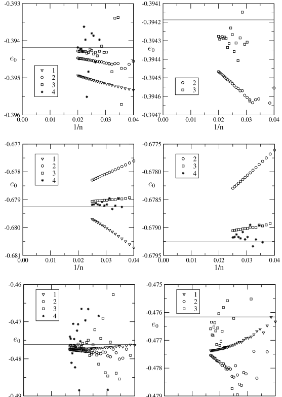
Figure 1: Estimates of the amplitude $e_{0}$ vs. $1/n$ for the square lattice (top panels), hexagonal lattice (middle panels) and triangular lattice (bottom panels).

We finally considered the amplitude combinations $e_{k}e_{1}^{-k}e_{0}^{k-1}$, where $2\leq k\leq 10$. They were estimated from the ratios

$$\frac{\Gamma(\beta_{k})[q^{n}]h^{(r)}_{k}(q)\left(\Gamma(\beta_{0})[q^{n}]h_{0}^{(r)}(q)\right)^{k-1}}{\left(\Gamma(\beta_{1})[q^{n}]h_{1}^{(r)}(q)\right)^{k}}\sim e_{k}e_{1}^{-k}e_{0}^{k-1}\qquad(n\to\infty).$$ (4.6)

We extracted the amplitudes by a direct fit to the expected asymptotic form, as explained in the appendix. As argued above, we fitted with exponents of the form $\alpha_{i}=(i+1)/3$ for $1\leq i\leq M_{0}$, where $2\leq M_{0}\leq 4$. The result is shown in Table 2. The prediction of the amplitude combinations appears to be correct, within numerical accuracy.

5 Unrooted self-avoiding polygons

The $k$th perimeter moment of rooted self-avoiding polygons $h_{k}^{(r)}(q)$ is related to the $(k+1)$th perimeter moment $h_{k+1}(q)$ of unrooted self-avoiding polygons. We have, for $k\geq 0$,

$$\begin{split}h_{k}^{(r)}(q)&=\left.\frac{(-1)^{k}}{k!}\frac{d^{k}}{dx^{k}}G^{(r)}(x,q)\right|_{x=x_{c}}=\left.\frac{(-1)^{k}}{k!}\frac{d^{k}}{dx^{k}}\left(x\frac{d}{dx}G(x,q)\right)\right|_{x=x_{c}}\\ &=\left.\frac{(-1)^{k}}{k!}\left(k\frac{d^{k}}{dx^{k}}G(x,q)+x\frac{d^{k+1}}{dx^{k+1}}G(x,q)\right)\right|_{x=x_{c}}\\ &=k\,h_{k}(q)-(k+1)\,x_{c}\,h_{k+1}(q)\sim-(k+1)\,x_{c}\,h_{k+1}(q)\qquad(q\to 1)\end{split}$$ (5.1)

The last relation follows with the exponents $\beta_{k}=2k/3-1/3$ of $h_{k}^{(r)}(q)$ given in (3.2). It follows from (5.1) that, for $k>0$, the singular behaviour of $h_{k}(q)$ is determined by the singular behaviour of $h_{k-1}^{(r)}(q)$. So we have all the moments of unrooted SAP except the zeroth moment. It thus remains to analyse the moment $h_{0}(q)$.

Extrapolating the values of $\beta_{k}$ to $k=-1$ gives $\beta_{-1}=-1$, so we expect a singularity of the form

$$h_{0}^{(sing)}(q)\sim A(1-q)\log(1-q)\qquad(q\to 1),$$ (5.2)

with some amplitude $A>0$. This behaviour was tested by a direct fit to the expected asymptotic form. Using the notation of the appendix, we expect an exponent $\alpha=-1$ and choose $\alpha_{i}=i$ for $1\leq i\leq M_{0}$, where $2\leq M_{0}\leq 4$ for stable approximation schemes.

For the square lattice, we find $c_{0}=0.026527(6)$. The numerical analysis yields $c_{0}=0.026527(3)$ on the hexagonal lattice, and $c_{0}=0.05306(5)$ on the triangular lattice. This suggests a universal law of the form

$$\sum_{m}p_{m,n}x_{c}^{m}\sim\frac{1}{6\pi\sigma}\frac{1}{n^{2}}\qquad(n\to\infty),$$ (5.3)

where $\sigma=2$ for the square lattice and the hexagonal lattice, and $\sigma=1$ for the triangular lattice. We have $1/(12\pi)=0.0265258...$ and $1/(6\pi)=0.0530516...$, which is, within error bars, in agreement with the estimates obtained above.

If one accepts the predicted scaling form (1.1) and scaling function (2.4) of rooted self-avoiding polygons, (and we believe that we have provided compelling numerical evidence to do so), then the scaling function of (unrooted) self-avoiding polygons is determined by integration,

$$G^{(sing)}(x,q)\sim(1-q)F\left(\frac{x_{c}-x}{(1-q)^{2/3}}\right)+C(q),\qquad(x,q)\to(x_{c},1),$$ (5.4)

where $C(q)$ is a “constant” of integration, given below, and $F(s)$ is given by

$$F(s)=\frac{4f_{1}}{x_{c}}\log\mbox{Ai}\left(\left(\frac{f_{0}}{4f_{1}}\right)^{2/3}s\right),$$ (5.5)

where the coefficients $f_{0}$ and $f_{1}$ are given in Table 1, and $x_{c}$ is given in the introduction. Alternatively, $F(s)$ can be expressed in terms of the amplitude $E_{0}$ given in Table 1 by

$$F(s)=-\frac{1}{\pi\sigma}\log\mbox{Ai}\left(\frac{\pi}{x_{c}}(2E_{0})^{2/3}s\right).$$ (5.6)

The term $C(q)$ incorporates the singular behaviour of the bicritical area generating function $h_{0}(q)=G(x_{c},q)$ as $q$ approaches unity, since the limit $x\to x_{c}$ from the other term yields a vanishing contribution. The function $C(q)$ is thus given by

$$C(q)=\frac{1}{6\pi\sigma}(1-q)\log(1-q).$$ (5.7)

The scaling form (5.4), (5.6) and (5.7) refines the prediction given previously in [22] by the addition of the term (5.7).

6 Crossover to branched polymer phase

Let $x_{c}(q)$ denote the radius of convergence of the perimeter and area generating function $G^{(r)}(x,q)$ of rooted SAP for $q<1$ fixed, as $q\to 1$. The scaling function prediction (1.1) leads to a prediction of the slope of the critical line $x_{c}(q)$, see also [2, 23]. The slope of the critical line is determined by the first singularity $s_{c}$ of the scaling function $H^{(r)}(s)$ on the negative real axis. More precisely, for $q<1$ fixed, the argument $s=(x_{c}-x)/(1-q)^{\phi}$ of the scaling function is negative for $x>x_{c}$, attaining its singular value $s_{c}$ for $x=x_{c}(q)>x_{c}$. We thus expect asymptotically

$$x_{c}(q)\sim x_{c}-s_{c}(1-q)^{\phi}\qquad(q\to 1).$$ (6.1)

For the particular scaling function (2.4), the point $s_{c}$ is given by

$$\left(\frac{f_{0}}{4f_{1}}\right)^{\frac{2}{3}}s_{c}=-2.3381074104\ldots$$ (6.2)

From the values of Table 1, we obtain $s_{c}=-0.2608637(5)$, $-0.2161405(20)$, and $s_{c}=-0.274509(2)$ for the square, hexagonal, and triangular lattices respectively. Note that, due to the particular form of the scaling function, the same behaviour applies to unrooted self-avoiding polygons.

Figure 2: Plots of $x_{c}(q)-x_{c}$ versus $1-q$ for the square lattice (top), hexagonal lattice (middle) and triangular lattice (bottom). The solid line has the predicted slope $2/3$.

Figure 2 displays a log-log plot of $x_{c}(q)-x_{c}$ versus $1-q$. In each plot a straight line corresponding to the expected form

$$x_{c}(q)-x_{c}=-s_{c}(1-q)^{2/3}$$ (6.3)

is given. We get reasonable agreement with the predicted form. The estimates were obtained using third order differential approximants [11], with the degree of inhomogeneous polynomial ranging from 5 to 15, and the requirement that averages must include at least $85\%$ of the approximants. For this part of our study we calculated the numbers $p_{m,n}$ for $m\leq 90$ (square lattice), $m\leq 134$ (hexagonal lattice) and $m\leq 50$ (triangular lattice), and all relevant sizes of the area.

If the scaling function $H^{(r)}(s)\sim a(s-s_{c})^{g}$ about $s=s_{c}$, it follows that the singular part of $G^{(r)}(x,q)$ behaves as $G^{(r),(sing)}(x,q)\sim a(1-q)^{-g\phi}(x_{c}(q)-x_{c})^{g}$ for $x\to x_{c}(q)$. The scaling function (2.4) has a simple pole at $s_{c}$ so

$$G^{(r),(sing)}(x,q)\sim a(1-q)^{2/3}(x_{c}(q)-x_{c})^{-1}.$$ (6.4)

The differential approximant analysis typically yields reasonably accurate exponent estimates for $q\leq 0.995$ and confirms that $G^{(r)}(x,q)$ has a simple pole as $x\to x_{c}(q)$. For example the analysis of the square lattice series yields $g=-1.0(3)$ at $q=0.995$, $g=-1.03(2)$ at $q=0.99$ and $g=-0.999(2)$ at $q=0.95$. For $q$ closer to 1 the exponent estimates became unreliable in that the errors bars were as large as the estimates, e.g. at $q=0.997$ we found $g=-1.6\pm 1.7$. We also tried to calculate the amplitude $a(q)\sim a(1-q)^{2/3}$, but unfortunately we could not get accurate estimates for $q>0.9$, and so have been unable to numerically confirm the predicted behaviour.

Finally, we checked the behaviour of the phase boundary $x_{c}(q)$ as $q\to 0$. The coefficient of $x^{m}$ in $G^{(r)}(x,q)$ is a polynomial in $q$ and as $q\to 0$ it becomes completely dominated by the term of lowest degree in $q$. We thus have to examine the behaviour of the terms $a_{m}=p_{m,n_{\rm min}}$, where $p_{m,n_{\rm min}}$ is the number of polygons with perimeter $m$ having the minimal possible area $n_{\rm min}$. Clearly, the polygon formed by making a linear chain of unit cells contributes to $a_{m}$. Unit cells on the square, hexagonal and triangular lattices have perimeter 4, 6 and 3, respectively, and it thus follows that $n_{\rm min}\simeq m/2$ (square), $m/4$ (hexagonal) and $m$ (triangular). On the square lattice it has been shown [9] that $a_{m}$ grows exponentially with $m$. $a_{m}$ is bounded from above by the number of site trees of size $n_{\rm min}$ on the dual lattice and from below by the number of minimally spanning polyominoes of size $n_{\rm min}$ (a minimally spanning polyomino is a polyomino spanning a $h\times w$ rectangle having size $h+w+1$). Similar arguments apply to the other lattices. So we form the generating function $S(t)=\sum_{m}a_{m}t^{m}$ and using differential approximants find that $S(t)$ has a singularity at $t_{c}=0.5189688(2)$ on the square lattice, $t_{c}=0.6986253(5)$ on the hexagonal lattice, and $t_{c}=0.346530(1)$ on the triangular lattice. Since $t^{m}=x^{m}q^{n_{\rm min}}$ it follows that $x_{c}(q)\sim t_{c}/q^{b}$, with $b=1/2$, $1/4$ and $1$ for the square, hexagonal and triangular lattice, respectively. Figure 3 shows a log-log plot of $x_{c}(q)$ versus $q$. In each plot a straight line corresponding to the expected form $x_{c}(q)=t_{c}/q^{b}$ is also shown.

Figure 3: Plots of $x_{c}(q)$ versus $q$ for the square lattice (top), hexagonal lattice (middle) and triangular lattice (bottom). The solid line has the predicted form $x_{c}(q)=t_{c}/q^{b}$ with slope $b=1/2$, $1/4$ and 1, respectively.

7 Conclusions

We have analysed bicritical perimeter moments of self-avoiding polygons using data obtained from exact enumeration on the square, hexagonal and triangular lattices. This yields a new check of the earlier scaling function conjecture for self-avoiding polygons. The numerical analysis supports the crossover behaviour of the critical line to the branched polymer regime. Whereas we find the scaling function conjecture for rooted self-avoiding polygons satisfied, it can be valid for unrooted self-avoiding polygons only in modified form. By analysing the bicritical area generating function, we suggest a modification by an additional term with an apparently universal amplitude, see (5.4), (5.6) and (5.7). It would be interesting to consider whether its value can be justified by field theoretical arguments; compare the related investigation [3].

Appendix: Numerical methods

We numerically analyse sequences $a_{n}$ by a direct fit to the expected asymptotic form. Similar applications of this method can be found in [14, 15]. The sequence $a_{n}$ is assumed to behave asymptotically as

$$a_{n}\sim\mu^{n}n^{\alpha-1}\left(c_{0}+\frac{c_{1}}{n^{\alpha_{1}}}+\frac{c_{2}}{n^{\alpha_{2}}}+\ldots+\frac{c_{M}}{n^{\alpha_{M}}}\right)\qquad(n\to\infty),$$ (7.1)

with constants $\mu>0$, $c_{i}\neq 0$ for $i=0,1,\ldots,M$, and exponents $\alpha$ and $\alpha_{i}$ for $i=1,\ldots,M$, where $\alpha_{i+1}>\alpha_{i}$ for $i=1,\ldots,M-1$. Estimates of the constant $\mu$ and the exponent $\alpha$ can be obtained by, e.g., the method of differential approximants [11]. We have $\mu=1$ in our examples. Often the sequence $(\alpha_{i})_{i=1}^{M}$ is unknown, but there are predictions for the numbers $\alpha_{i}$. The validity of a prediction can be tested employing the following procedure:

We perform a direct fit to the expected asymptotic form, i.e., we solve the linear system

$$a_{n}=\mu^{n}n^{\alpha-1}\left(d_{0}+\frac{d_{1}}{n^{\alpha_{1}}}+\frac{d_{2}}{n^{\alpha_{2}}}+\cdots+\frac{d_{M}}{n^{\alpha_{M}}}\right)\qquad(n=N-(M+1),\ldots,N)$$ (7.2)

for the $M+1$ unknowns $d_{i}$. If the assumption of the asymptotic form (7.1) is correct, then the numbers $d_{i}=d_{i}(N,M)$ will satisfy

$$d_{i}(N,M)\to c_{i}\qquad(N\to\infty).$$ (7.3)

Generally, if the wrong sequence has been chosen, the sequence of coefficients $d_{i}(N,M)$, for increasing values of $N$ and fixed $M$, diverges either to infinity or converges to zero; but if the correct sequence has been chosen, convergence is usually rapid and obvious.

Let us fix $i$ in the following. Estimates of the amplitudes $c_{i}$ are obtained in the following way. For $N$ large enough, the numbers $d_{i}(N,M)$ display approximately linear variation in $1/N$,

$$d_{i}(N,M)\sim c_{i}(M)+\frac{r_{i}(M)}{N}\qquad(N\to\infty).$$ (7.4)

The numbers $c_{i}(M)$ are obtained by a linear least squares fit of $d_{i}(N,M)$ for large values of $N$. The larger $M$, the larger $N$ has to be taken in order to reach the asymptotic regime (7.4). Since, however, $N\leq N_{0}$ for given series data, $d_{i}(N,M)$ is close to the asymptotic regime only for values of $M\leq M_{0}$, where $M_{0}$ has to be extracted from series analysis. We choose $1\leq m_{0}\leq M_{0}$ such that $|r_{i}(m_{0})|$ is minimal. We estimate $c_{i}$ by $c_{i}(m_{0})$ and estimate the error by the spread among different values $c_{i}(m)$ for $1\leq m\leq M_{0}$.

The amplitudes $c_{i}$ in (7.1) are related to the critical amplitudes of the corresponding generating functions. If $\alpha\notin-\mathbb{N}_{0}$, the singular amplitude $B$ of the corresponding generating function

$$A(x)=\sum_{n=0}^{\infty}a_{n}x^{n}\sim A^{(reg)}(x)+\frac{B}{(\mu^{-1}-x)^{\alpha}}\qquad(\mu x\to 1)$$ (7.5)

is related to $c_{0}$ via $B=c_{0}\Gamma(\alpha)\mu^{-\alpha}$.

References

- [1] Cardy J L 1994 Mean area of self-avoiding loops Phys. Rev. Lett. 72 1580–1583; cond-mat/9310013
- [2] Cardy J L 2001 Exact scaling functions for self-avoiding loops and branched polymers J. Phys. A: Math. Gen. 34 L665–L672; cond-mat/0107223
- [3] Cardy J L and Ziff R M 2003 Exact results for the universal area distribution of clusters in percolation, Ising and Potts models J. Stat. Phys. 110 1–33; cond-mat/0205404
- [4] Duchon P 1999 -grammars and wall polyominoes Ann. Comb. 3 311–321
- [5] Enting I G 1980 Generating functions for enumerating self-avoiding rings on the square lattice J. Phys. A: Math. Gen. 13 3713–3722
- [6] Enting I G and Guttmann A J 1989 Polygons on the honeycomb lattice J. Phys. A: Math. Gen. 22 1371–1384
- [7] Enting I G and Guttmann A J 1990 On the area of square lattice polygons J. Stat. Phys. 58 475–484
- [8] Enting I G and Guttmann A J 1992 Self-avoiding rings on the triangular lattice J. Phys. A: Math. Gen. 25 2791–2807
- [9] Fisher M E Guttmann A J and Whittington S G 1991 Two-dimensional lattice vesicles and polygons J. Phys. A: Math. Gen. 24 3095–3106
- [10] Flajolet P and Louchard G 2001 Analytic variations on the Airy distribution Algorithmica 31 361–377
- [11] Guttmann A J 1989 Asymptotic analysis of power-series expansions in: Phase Transitions and Critical Phenomena vol. 13 eds Domb C and Lebowitz J (London: Academic Press) 1–234
- [12] Janse van Rensburg E J 2000 The Statistical Mechanics of Interacting walks, Polygons, Animals and Vesicles (New York: Oxford University Press)
- [13] Janse van Rensburg E J 2004 Inflating square and rectangular lattice vesicles J. Phys. A: Math. Gen. 37 3903–3932
- [14] Jensen I and Guttmann A J 1999 Self-avoiding polygons on the square lattice J. Phys. A: Math. Gen. 32 4867–4876; cond-mat/9905291
- [15] Jensen I 2003 A parallel algorithm for the enumeration of self-avoiding polygons on the square lattice J. Phys. A: Math. Gen. 36 5731–5745; cond-mat/0301468
- [16] Lawler G F Schramm O and Werner W 2002 On the scaling limit of planar self-avoiding walk preprint; math.PR/0204277
- [17] Madras N and Slade G 1993 The Self-Avoiding Walk (Boston: Birkhäuser)
- [18] Nienhuis B 1982 Exact critical point and critical exponents of O() models in two dimensions Phys. Rev. Lett. 49 1062–1065
- [19] Prellberg T 1995 Uniform -series asymptotics for staircase polygons J. Phys. A: Math. Gen. 28 1289–1304
- [20] Prellberg T and Brak R 1995 Critical exponents from non-linear functional equations for partially directed cluster models J. Stat. Phys. 78 701–730
- [21] Prellberg T and Owczarek A L 1995 Partially convex lattice vesicles: methods and recent results Proc. Conf. on Confronting the Infinite (Singapore: World Scientific) 204–214
- [22] Richard C Guttmann A J and Jensen I 2001 Scaling function and universal amplitude combinations for self-avoiding polygons J. Phys. A: Math. Gen. 34 L495–L501; cond-mat/0107329
- [23] Richard C 2002 Scaling behaviour of two-dimensional polygon models J. Stat. Phys. 108 459–493; cond-mat/0202339
- [24] Richard C Jensen I and Guttmann A J 2003 Scaling function for self-avoiding polygons in: Proceedings of the International Congress on Theoretical Physics TH2002 (Paris) eds Iagolnitzer D Rivasseau V and Zinn-Justin J (Basel: Birkhäuser), Supplement, pp. 267–277; cond-mat/0302513
- [25] Richard C 2004 Area distribution of the planar random loop boundary J. Phys. A: Math. Gen. 37 4493–4500; cond-mat/0311446