A statistical theory of nucleation in the presence of uncharacterised impurities

Abstract

First order phase transitions proceed via nucleation. The rate of nucleation varies exponentially with the free-energy barrier to nucleation, and so is highly sensitive to variations in this barrier. In practice, very few systems are absolutely pure, there are typically some impurities present which are rather poorly characterised. These interact with the nucleus, causing the barrier to vary, and so must be taken into account. Here the impurity-nucleus interactions are modelled by random variables. The rate then has the same form as the partition function of Derrida’s Random Energy Model, and as in this model there is a regime in which the behaviour is non-self-averaging. Non-self-averaging nucleation is nucleation with a rate that varies significantly from one realisation of the random variables to another. In experiment this corresponds to variation in the nucleation rate from one sample to another. General analytic expressions are obtained for the crossover from a self-averaging to a non-self-averaging rate of nucleation.

I Introduction

Nucleation has long been known to be very sensitive to impurities. Very pure water can be cooled to tens of degrees below freezing, 0C at atmospheric pressure, before it crystallises, but in practice the water in our freezers freezes at only a little below 0C debenedetti . The crystals of ice in our freezer presumably nucleate heterogeneously, in contact with some unknown impurity in the water. The nucleus of water may be only a few water molecules across and so is only a nanometer or so across. Thus, even impurities only a nanometer across can interact with the nucleus and so greatly reduce the free-energy barrier to nucleation. The impurity may of course be much larger. Often we know little of the impurity that is providing a surface where the nucleus of ice can form at a much lower free-energy cost than in the bulk. Here, we circumvent the problem that the impurities are typically uncharacterised, by using a statistical theory. We address the question: Under what conditions can chance variations from sample to sample in the impurities present, cause the nucleation rate to vary significantly from sample to sample? That is we develop a theory that links an observable, the variability of nucleation rate, with the variability of the impurities at microscopic length scales.

Given the ubiquitous nature of this problem of heterogeneous nucleation occurring on uncharacterised impurities, relatively little theoretical work has been done. Karpov and Oxtoby karpov94 ; karpov96 have considered nucleation in the presence of random static disorder, and Harrowell and Oxtoby harrowell93 looked at the effect of the distribution of time scales present in glasses. But this work did not address the problem of sample to sample variability, and little theoretical work has been done for a number of years. Castro and coworkers castro99 ; castro03 studied the process that follows nucleation, namely growth. See also Ref. karpov95 . The pattern of growth depends on whether nucleation occurs continuously throughout the process of phase transformation or only at a few sites near the start of the process. We find sample to sample variability occurs when one or a few sites have unusually low nucleation barriers and so there should be a correlation between the pattern of growth (and hence the final distribution of grain sizes if the new phase forming is crystalline) and sample to sample variability in the nucleation rate. Castro and coworkers consider only growth, they did not explicitly consider nucleation, and they did not consider sample to sample variability.

Just as Karpov and Oxtoby did karpov96 , we will consider nucleation in the presence of disorder. We will model the system as a nucleus interacting with random disorder, i.e., the free energy of the nucleus will contain a part that is a random variable. Essentially, faced with a situation where we know the free energy barrier to nucleation depends on its interaction with species unknown, we realise that it is not possible to base a theoretical description on precise knowledge and make a plausible simple guess. Individual interactions are modelled by random variables with some mean and standard deviation and the system is then characterised just by these two numbers.

The rate of nucleation at a site is proportional to the exponential of minus the free-energy divided by the thermal energy $k_{B}T$. See the book of Debenedetti debenedetti or the review of Oxtoby oxtoby92 or of Kashchiev and van Rosmalen kashchiev03 for an introduction to nucleation. Thus the rate at a particular site is proportional to the Boltzmann factor of the nucleus at that site and so a sum over different sites with different free-energy barriers has the form of a sum over Boltzmann weights. This is of course the form of a partition function; a partition function of a system where the energies are random variables. Such a system is called the Random Energy Model (REM) and was first proposed and studied by Derrida derrida80 . He was using it as a simple model for a glass. We can take over much of the analysis of the REM done by Derrida and apply it to our system. Most importantly, at low temperatures the REM is not self-averaging: different realisations of the disorder give rise to significantly different partition functions. In our system the analogue of the partition function of the REM is the total rate of nucleation, and different realisations correspond to different samples prepared in the same conditions. So, we have a regime in which the rate is not self-averaging: it differs significantly from sample to sample. Note that this is distinct from variability in properties such as the time until the first nucleus appears. As the crossing of a nucleation barrier is a random process the time it takes will always be a random variable, but if there is little or no variability in the free-energy barrier the rate itself will self-average and so not vary from sample to sample. Having recognised that our problem is isomorphic to Derrida’s REM we have a model for the experimental observation of sample-to-sample variability. This model allows us to obtain quantitative relations between the width of the distribution of the free-energy barriers to nucleation, the number of nucleation sites, and the sample-to-sample variability.

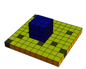
Figure 1: (Colour online) Schematic representation of a nucleus represented by a 3 by 3 by 3 cube of dark blue monomers, in contact with a flat surface composed of 2 types of monomers: light and dark yellow.

The next section is a very general study of nucleation with a free energy barrier that contains a term that is a random variable. The number of nucleation sites $N_{s}$ is fixed, although our theory can be generalised to deal with varying amounts of impurity nucleation sites, see section II.2. Section III is devoted to the study of an explicit model of a disordered system: a surface composed of two types of monomers that are distributed at random. Figure 1 is a schematic of this model. We show how this random distribution of monomers leads to a random term in the free energy of a nucleus in contact with the surface and obtain an explicit expression for the width $w$ of the distribution of free-energy barriers. The model of Fig. 1 is just one possible system that results in a random term in the free-energy barrier to nucleation, we can envisage many others. Indeed other activated processes with the same exponential dependence on the height of a free-energy barrier, such as protein unfolding searunf , have essentially the same behaviour in the presence of disorder. Disorder can be a model not only for uncharacterised impurities but also for very complex environments such as that inside a living cell. Section IV outlines the use of Bayes’s theorem to estimate the nucleation rate from a small number of observations of nucleation. This is useful as if the nucleation rate can be estimated for two different samples and shown to be different in these two samples, the experimental system must be in the non-self-averaging regime. The last section is a conclusion.

II General theory

Nucleation is an activated process debenedetti ; oxtoby92 ; kashchiev03 . As such, its rate has an exponential dependence on the free-energy barrier to nucleation, $\Delta F^{*}$, the free-energy of the critical nucleus. The critical nucleus is, by definition, the nucleus at the top of the barrier to nucleation debenedetti . Thus, if at site $i$ of the system, the free energy barrier is $\Delta F^{*}_{i}$, and the frequency of attempts at unfolding is $\nu_{i}$, then the rate of nucleation at the site $i$ is

$$R_{i}=\nu_{i}\exp\left(-\Delta F^{*}_{i}\right).$$ (1)

We will assume that the attempt frequency $\nu_{i}$ is only weakly dependent on $i$ and so treat it as a constant: $\nu_{i}=\nu$. As $\Delta F^{*}_{i}$ is exponentiated, if it varies appreciably then its variation dominates that of $\nu_{i}$ which can then be neglected. We use units such that the thermal energy $k_{B}T=1$. If the system consists of $N_{s}$ possible sites for nucleation then the average nucleation rate per site is simply

$$R = N_{s}^{-1}\sum_{i=1}^{N_{s}}R_{i}$$ (2)

$$= N_{s}^{-1}\nu\sum_{i=1}^{N_{s}}\exp\left(-\Delta F^{*}_{i}\right).$$ (3)

Thus to calculate the nucleation rate we require the $N_{s}$ values of the nucleation barrier at all possible nucleation sites.

Often, the system of interest is complex, or poorly characterised with unknown impurities present. Then, we have little hope of determining all the $N_{s}$ values of $\Delta F^{*}_{i}$. To deal with these situations we resort to a statistical approach: we guess the values of $\Delta F^{*}_{i}$. We do this by picking the $\Delta F^{*}_{i}$ from a probability distribution function that is characterised by two parameters, its mean $m$ and standard deviation $w$. These two parameters can in turn be obtained from a model, estimated from experimental data, or simply varied to see what qualitative behaviour is possible. We estimate them from a specific model in section III.

It is convenient to express the $\Delta F^{*}_{i}$ as a mean plus a deviation,

$$\Delta F^{*}_{i}=m+\delta_{i},$$ (4)

where $\delta_{i}$ is a random variable with zero mean, it is the deviation of the nucleation barrier at site $i$ from its mean value $m$. Taking the probability distribution of $\delta_{i}$, $p(\delta_{i})$, to be a Gaussian, we have

$$p(\delta_{i}) = \frac{\exp\left[-\delta_{i}^{2}/(2w^{2})\right]}{\left(2\pi w^{2}\right)^{1/2}}.$$ (5)

Using Eq. (4) for $\Delta F^{*}_{i}$ we can write Eq. (3) as

$$R=N_{s}^{-1}\nu\exp(-m)\sum_{i=1}^{N_{s}}\exp\left(-\delta_{i}\right).$$ (6)

Now, with the $\Delta F^{*}_{i}$ independent random variables, the rate of Eq. (6) is, except for constant factors, equivalent to the partition function of the Random Energy Model (REM) of Derrida derrida80 . The REM is a simple and well understood model of glasses and other disordered systems that undergo a transition to a state that is non-self-averaging.

Just as in the REM the average partition function can be obtained, we can obtain the average, over realisations of the disorder, of the nucleation rate $R$,

$$\langle R\rangle = N_{s}^{-1}\nu\exp\left(-m\right)\langle\sum_{i=1}^{N_{s}}\exp\left(-\delta_{i}\right)\rangle$$ (7)

$$= \nu\exp\left(-m+w^{2}/2\right).$$ (8)

If the rate $R$ is self-averaging then for almost all realisations $R$ will be close to $\langle R\rangle$ and the right-hand side of Eq. (8) will be a good approximation to the nucleation rate of almost all realisations of our model of the surfaces inside a cell. But if the rate $R$ is not self-averaging then Eq. (8) will not be a good approximation and the rate $R$ will differ appreciably from one realisation to another. Nucleation in the presence of random static disorder was considered by Karpov and Oxtoby karpov96 who obtained results similar to that of Eq. (8), but they only considered self-averaging systems.

II.1 Measures of non-self-averaging behaviour

We will now look at how as the width of the distribution of free-energy barriers, $w$, increases the behaviour ceases to be self-averaging. Firstly, we will look at how many nucleation sites contribute significant amounts to the nucleation rate in a typical realisation. If this number is large then as the sites are assumed independent the rate is a sum of a large number of independent random variables and so will be self-averaging, whereas if it is small this will not be the case.

From Eq. (6) we see that the rate $R$ is dominated by sites with values of $n_{i}$ where the product of the number of sites and $\exp(-\delta_{i})$, is a maximum. The number of sites is simply proportional to the probability of Eq. (5). The maximum of the product $p(\delta_{i})\exp(-\delta_{i})$ is at a value of $\delta$,

$$\delta_{max}=-w^{2}.$$ (9)

Now, the average number of sites around this value of $\delta_{i}$ is just $N_{s}p(\delta_{max})$, and because this average is a sum over independent random variables (the $n_{i}$) the ratio of the fluctuations to the mean scales as $[N_{s}p(\delta_{max})]^{-1/2}$. Thus the fluctuations in the number of sites that contribute the dominant amount to the rate, and hence the fluctuations in the rate itself are small relative to the mean if and only if $N_{s}p(\delta_{max})\gg 1$. From Eqs. (5) and (9) this is true whenever $2\ln N_{s}-w^{2}>0$.

Thus, the boundary between self-averaging and non-self-averaging regimes is given by the equation

$$2\ln N_{s}-w^{2}=0.$$ (10)

Thus the rate is self-averaging if and only if the logarithm of the number of possible sites for nucleation, is larger than half the variance of the nucleation barrier. This is the main result of this work. It is a very general result, i.e., it applies generally to activated processes in a random or near-random environment. Our conclusions here apply to any process with a rate given by an equation of the form of Eq. (3). In the next section we will give the example of heterogeneous nucleation at a disordered surface and in Ref. searunf , we showed that it held for a model of protein unfolding in vivo.

In the non-self-averaging regime, a single unfolding site can be responsible for a significant fraction of the entire rate. This site must of course be the site with the lowest, i.e., most negative, value of $\delta_{i}$. We denote this lowest value by $x$. We can easily find an estimate for $x$, which we call $\delta_{ev}$. It is simply the value of $\delta$ at which the mean number density, $N_{s}p(\delta_{i})$, of sites drops below 1. This is easy to see: it cannot be much below the value of $\delta$ for which $N_{s}p(\delta)\approx 1$ as there are rarely any sites at all below this value and it cannot be much above it as for these values of $\delta$ there are many sites. Thus, we have that $\delta_{ev}$ satisfies the equation $N_{s}p(\delta_{ev})=1$, and so is given by

$$\delta_{ev}=-\left(2\ln N_{s}\right)^{1/2}w,$$ (11)

where to obtain this result we ignored the denominator of Eq. (5).

So when a single site dominates the rate $R$, and has a value of $\delta_{i}$ close to $\delta_{ev}$, the rate is approximately

$$R_{T}\simeq N_{s}^{-1}\nu\exp\left(-m+\left(2\ln N_{s}\right)^{1/2}w\right),$$ (12)

using Eq. (11) in Eq. (6). Note that $R_{T}\ll\langle R\rangle$ for large widths; $\langle R\rangle$ increases as the exponential of $w^{2}$, Eq. (8), whereas $R_{T}$ increases as only the exponential of $w$. Equation (9) tells us that at, for example $w=6$ the maximum contribution to the average rate, $\langle R\rangle$, comes from sites with values of $\delta$ around $\delta_{max}=36$. At these values of $\delta$ the probability density, Eq. (5) is close to $10^{-9}$. Thus even for $N_{s}=10^{8}$ there is on average less than one site at values of $\delta$ close to $\delta_{max}$. For $N_{s}=10^{8}$ most realisations have no sites around $\delta_{max}=36$, and so have values of $R$ rather less than its mean value $\langle R\rangle$, and closer to $R_{T}$. The large value of $\langle R\rangle$ is due to a few realisations with very large values of $R$.

Our analysis started with Eq. (1), the standard expression for the rate of a barrier-crossing process. This is only valid if there is a barrier to cross, i.e., if $m+\delta_{i}$ is at least a few $k_{B}T$. If there are sites present for which $m+\delta_{i}$ is close to zero, which is true if $m-(2\ln N_{s})^{1/2}w\lesssim 0$ (Eq. (11)), then the nucleation rate at these sites will be essentially $\nu$. In this case we would expect these sites to dominate the nucleation rate as nuclei form effectively immediately at these sites. The rate will then be self-averaging if and only if the average number of these sites in a sample is much larger than one. In the remainder of the manuscript we will assume that $m-(2\ln N_{s})^{1/2}w$ is at least a few $k_{B}T$.

Also, Eq. (12) is for the rate when it is dominated by a single site. We would expect that often when nucleation has occurred at a site the growing domain of the nucleated phase will prevent the formation of further nuclei at this site. If this is so then once the first nucleus has formed then the rate $R$ will decrease as then only the other sites with higher free-energy barriers to nucleation will remain. Thus associated with non-self-averaging nucleation rates we expect rates that are time dependent. When the rate $R$ contains contributions from many sites, clearly the rate will only decrease after many nuclei have formed and so any time dependence will be much less noticeable. The rates $R$ considered here are therefore initial rates. As determining the time dependence of rates requires study of the behaviour of nuclei after they have crossed the barrier we do not consider this time dependence here, although see Refs. castro99 ; castro03 for post-nucleation growth in systems with distributions of nucleation barriers.

We will now perform a quantitative analysis of the fraction of the rate due to the site with the lowest free-energy barrier, i.e., due to the one with $\delta_{i}=x$. We calculate the average, $f_{ev}$, of the fraction of the rate due to the site with the lowest free-energy barrier. This can be calculated from the probability distribution function, $p_{ev}(x)$, using

$$f_{ev}=\frac{\nu\exp\left(-m\right)}{N_{s}\langle R\rangle}\int p_{ev}(x)\exp\left(-x\right){\rm d}x.$$ (13)

We can simplify Eq. (13) by introducing the reduced variable $y=x/w$. Then, from Eq. (13) and using Eq. (8) for $\langle R\rangle$, we obtain

$$f_{ev}=N_{s}^{-1}\exp\left(-w^{2}/2\right)\int{\rm d}yp_{ev}(y)\exp\left(-wy\right),$$ (14)

where $p_{ev}(y)$ is the probability distribution function for the minimum value of a set of $N_{s}$ values taken from a Gaussian of zero mean and unit standard deviation. Note that although the absolute value of the rate $R$ and of the contribution of the extreme value both depend on the mean $m$, $f_{ev}$ does not. It depends only on $w$, and $N_{s}$.

The determination of $p_{ev}(y)$ is a standard problem in extreme-value statistics sornette . We start from the fact that the probability that the minimum of $N_{s}$ values is $y$ is the probability that 1 of the $N_{s}$ sites has a value $y$, and all the remaining $N_{s}-1$ sites have larger values, multiplied by $N_{s}$, as any one of the $N_{s}$ sites can have the lowest value. Thus,

$$p_{ev}(y)=N_{s}p(y)p_{>}^{N_{s}-1}(y),$$ (15)

where $p(y)$ is a normalised Gaussian of zero mean and unit standard deviation, and $p_{>}(y)$ ($p_{<}(y)$) is the probability of obtaining a number larger (lower) than $y$ from a Gaussian of zero mean and unit standard deviation. We are interested in the region where $x$ is several standard deviations below the mean, $y\ll-1$. Now, $p_{>}=1-p_{<}$, and so as for $y\ll-1$, $p_{<}\ll 1$, we can rewrite Eq. (15) as

$$p_{ev}(y)\simeq N_{s}p(y)\exp\left[-N_{s}p_{<}(y)\right],$$ (16)

where we replaced $N_{s}-1$ by $N_{s}$. Also, $p_{<}(y)=(1/2)\mbox{erfc}(-y/2^{1/2})$, which for $y\ll-1$ simplifies to

$$p_{<}(y)\simeq\exp\left(-y^{2}\right)/[(2\pi)^{1/2}(-y)].$$ (17)

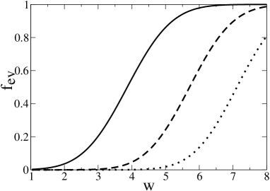
Figure 2: The mean fraction, $f_{ev}$, of the rate $R$ that is due to the site with the lowest $\delta_{i}$, as a function of the width of the Gaussian, $w$. The solid, dashed and dotted curves are for $N_{s}=10^{4}$, $10^{8}$ and $10^{12}$ sites, respectively.

In Fig. 2 we have plotted the fraction of the rate due to the site with the lowest barrier, $f_{ev}$, as a function of $w$. We took $N_{s}=10^{4}$, $10^{8}$ and $10^{12}$. For protein crystallisation durbin96 distinct sites should be at least 1nm apart. Then $N_{s}=10^{8}$ sites corresponds to a surface of order 100$\mu$m². The dependence on $N_{s}$ is logarithmic, varying $N_{s}$ by orders of magnitude does not have a marked effect. $\ln N_{s}$ should nearly always be of order 10. We see that as $w$ increases, so does $f_{ev}$. For $N_{s}=10^{8}$, Eq. (10) is satisfied for $w=6.07$. For $w$ around this value the site with the largest interaction energy already contributes a large amount to the total rate, on average. This large contribution will vary significantly from one realisation to the next, and so the fraction of the rate due to the site with the lowest value of the nucleation barrier will vary substantially from realisation to realisation at large $w$. For some realisations it will be rather larger than $f_{ev}$ and for others it will be much smaller. Whereas of course if $w$ is small the rate $R$ has significant contributions from many unfolding sites and so varies weakly from realisation to realisation, essentially due to variations in the rate being averaged out in accordance with the central-limit theorem.

II.2 Variable $N_{s}$

There is data on the effect of impurities from the work of Turnbull turnbull50 and coworkers, and that of Perpezko perpezko84 coworkers on nucleation from dispersions of liquid droplets debenedetti ; oxtoby92 . These experiments were motivated by the idea that if sufficiently small droplets could be formed some droplets would be free of all impurities and in those droplets the nucleation would then be homogeneous. It is not clear that this objective was achieved debenedetti ; oxtoby92 ; perpezko84 . Perpezko perpezko84 assumed that the impurities are randomly distributed, and then the number of impurity particles in a droplet is given by a Poisson distribution function. He addressed the question of random variation in the number of impurity particles but not that of variation in the interaction of the impurity with the nucleus. Thus in a sense it is complementary to this work. If we make the number of sites $N_{s}$ itself a random variable but set $w=0$ then we obtain the model of Perpezko perpezko84 . Thus if we allow the number of nucleation sites $N_{s}$ to be a random variable while maintaining $w$ non-zero we have a model that can describe both variation in both the number of impurity particles and disorder in the surface of these particles. We leave such a generalisation to future work.

III Disordered surfaces

In the previous section we merely assumed that the presence of disorder introduced a random part $\delta_{i}$ into the nucleation barrier at site $i$, and that the $\delta_{i}$ are drawn from a Gaussian distribution. In this section we will start from a simple model of a disordered surface and show that in a certain limit, a Gaussian distribution of free-energy barriers is obtained, and obtain expressions for the mean $m$ and width $w$, of this Gaussian, in terms of the parameters that characterise the surface.

Surfaces, for example of impurities, can provide sites for nucleation. We consider a simple planar surface formed of a plane of sites of a cubic lattice all occupied by fixed monomers. The nucleus is taken to be a block of monomers of single type which may be the same type as some of those of the surface or different. We assume that not more than one monomer can occupy a site, thus the nucleus can be in contact with the surface and so interact with it but it cannot penetrate the surface. Apart from this excluded-volume interaction, the only interactions are those between monomers in contact. If the surface were uniform, i.e., composed exclusively of one type of monomer then the free energy barrier to nucleation would of course be the same at every point on the surface. However, if the surface is composed of 2 types of monomers that are not uniformly distributed then the barrier will vary from point to point, depending on the numbers of monomers of the different types that the nucleus is in contact with at a particular point. A schematic of a cubic nucleus in contact with such a surface is shown in Fig. 1.

Let us call the 2 types of monomer A and B, and assume they are distributed at random. Let monomers of type $A$ and $B$ interact with the nucleus with energies $\epsilon_{A}$ and $\epsilon_{B}$, respectively. Then the shift in the barrier to nucleation when the nucleus is at a site $i$ in contact with the surface is

$$\Delta F^{*}_{i}=\Delta F^{*}_{0}+n_{i}\epsilon_{A}+(n_{c}-n_{i})\epsilon_{B},$$ (18)

where $\Delta F^{*}_{0}$ is the nucleation barrier when the the nucleus is not in contact with the surface. $n_{c}$ is the total number of sites in the nucleus that contact the surface; as the surface is taken to be planar this number is taken to be a constant. $n_{i}$ is the number of A monomers of the surface in contact with the nucleus when the nucleus is at site $i$. If the monomers of the surface are either A or B at random, then the probability of any one of the $n_{c}$ sites of the surface being an A-type monomer is just the fraction of A-type monomers, which we denote by $f_{A}$. Then the probability of the nucleus being in contact with $n_{i}$ A-type monomers and $n_{c}-n_{i}$ B-type monomers is just

$$p_{A}(n_{i}) = \frac{n_{c}!}{n_{i}!(n_{c}-n_{i})!}f_{A}^{n_{i}}\left(1-f_{A}\right)^{n_{c}-n_{i}}$$ (19)

$$\simeq \frac{\exp\left[-(n_{i}-m_{s})^{2}/(2w_{s}^{2})\right]}{\left(2\pi w_{s}^{2}\right)^{1/2}},$$ (20)

where the mean value $m_{s}=f_{A}n_{c}$, and the variance of the Gaussian $w_{s}^{2}=n_{c}f_{A}(1-f_{A})$.

Using Eqs. (4), (18) and (20) we see that the Gaussian distribution for $n_{i}$ becomes a Gaussian distribution for $\delta_{i}$ of variance

$$w^{2} = w_{s}^{2}\left(\epsilon_{A}-\epsilon_{B}\right)^{2}$$ (21)

$$= n_{c}f_{A}\left(1-f_{A}\right)\left(\epsilon_{A}-\epsilon_{B}\right)^{2}.$$

The mean value of the $\Delta F^{*}_{i}$ of Eq. (4) is

$$m=\Delta F^{*}_{0}+n_{c}(f_{A}\epsilon_{A}+(1-f_{A})\epsilon_{B}).$$ (22)

For the nucleation rate to be non-self-averaging we require that $w^{2}$ be larger than $2\ln N_{s}$, Eq. (10). Unless $N_{s}$ is extremely large or small $2\ln N_{s}$ will be of order 10. From Eq. (21) we see that if the difference in interaction energy between the 2 types of monomer, $\epsilon_{A}-\epsilon_{B}$ is a few $k_{B}T$, and if we have around $n_{c}=10$ sites of the surface in contact with the nucleus, then $w^{2}$ will be around 10 to 30, providing that $f_{A}$ is neither very small nor close to unity. Thus, we predict that heterogeneous nucleation at disordered surfaces composed of significant fractions of different species whose interactions with the nucleus differ by a few $k_{B}T$, will often be dominated by one or a few sites. It will therefore vary appreciably between realisations. Experimentally, this means that the rate will differ appreciably between nominally identical samples.

Finally, for the purposes of comparison we consider adsorption onto the surface of individual monomers. These monomers are of the same type as those that made up the nucleus. For simplicity we do so in the regime where we have much less than a monolayer, i.e., where the number of adsorbed monomers $\Gamma\ll N_{s}$. Now, we can compare the rate $R$ with the adsorbed amount $\Gamma$ in order to get a feel for which property is more likely to be non-self-averaging. When $\Gamma\ll N_{s}$ then few pairs of adjacent sites are occupied and so we can treat each surface site as being independent. Then $\Gamma$ is given by

$$\Gamma=\sum_{i=1}^{N_{s}}\frac{\exp\left[\mu+n_{i}\epsilon_{A}+(1-n_{i})\epsilon_{B}\right]}{1+\exp\left[\mu+n_{i}\epsilon_{A}+(1-n_{i})\epsilon_{B}\right]},$$ (23)

where $n_{i}=1$ if the monomer at site $i$ on the surface is an A-type monomer and $n_{i}=0$ if the monomer is a B-type monomer. $\mu$ is the chemical potential of the monomers (in units of $k_{B}T$). The variation of $\Gamma$ from realisation to realisation will depend on $\epsilon_{A}$, $\epsilon_{B}$, $f_{A}$ and $\mu$.

However, this variability simply comes from the fact that the terms in the sum of Eq. (23) take one of two values depending on whether the monomer is type A or type B. These two values are bounded by zero and one. Thus we can easily obtain an upper bound for this variation in $\Gamma$ by assuming the terms in the sum for $\Gamma$, Eq. (23) are either zero or one. This corresponds to, say, the A-type monomers always having a monomer adsorbed onto them while the B-type monomers never have an adsorbed monomer. For definiteness we assume that A-type monomers are the ones with adsorbed monomers. This approximation will clearly overestimate the variability in $\Gamma$ but even within this approximation the variance of $\Gamma$ is just $f_{A}(1-f_{A})N_{s}$ for large $N_{s}$. The ratio of the standard deviation to the mean, $f_{A}N_{s}$, is then given by

$$\frac{\mbox{std. dev.}}{\mbox{mean}}=\left(\frac{1-f_{A}}{f_{A}}\right)^{1/2}N_{s}^{-1/2}$$ (24)

and so is small for large $N_{s}$ and $f_{A}=O(0.1)$. At least when the adsorption is small $\Gamma$ is self-averaging. So disorder large enough to cause the rate $R$ to be non-self-averaging may leave other properties, e.g., $\Gamma$, still self-averaging. As the nucleus is large, $n_{c}=O(10)$, the variance in the free-energy barrier at a site is large (it is multiplied by $n_{c}$ in Eq. (21)) and the rate $R$ is then proportional to the exponential of this large quantity. Both the factor of $n_{c}$ and the exponentiation strongly enhance the effect of disorder and make the nucleation rate one of the most likely properties of a system to be non-self-averaging.

IV Determining the nucleation rate using Bayesian inference

In this section we will discuss the use of Bayesian inference to determine the probable nucleation rate from measurements of nucleation, and hence determine whether or not two (or more) different samples have the same or different nucleation rates. This is required as observing the effects of disorder on nucleation is hampered by the fact that nucleation is inherently a random process. There is more than one way to study nucleation and inference should be applicable to all of them, but for definiteness and because our nucleation rates $R$ are initial nucleation rates we study determining the rate of nucleation from the time until the first nucleus appears. Fortunately, the inference problem we need to solve is the same as that given and solved as an example in chapter 3 of the textbook of MacKay mackay . We shall therefore give only a brief presentation, referring the reader for details to Ref. mackay .

Nucleation is due to a fluctuation and so is random even in a completely uniform pure system. The time $t$ at which the first nucleus appears is a random variable. The probability distribution function for $t$ is an exponential,

$$p(t)=RN_{s}\exp\left(-RN_{s}t\right).$$ (25)

Experiments can also involve counting the number of events, and if these events are independent this number is given by a Poisson distribution function. For example Galkin and Vekilov galkin99 ; vekilov03 count the number of protein crystals formed. The analysis here can also be applied to determine whether or not two Poisson distributions have different means. If they have then that too indicates a varying nucleation rate.

Let us consider the situation where we have two samples that have been prepared in the same way. If we can determine that they have different nucleation rates then clearly we must be in the non-self-averaging regime whereas if we examine a number of samples and they all have indistinguishable rates then we are in the self-averaging regime. A given sample will have some unknown total nucleation rate $RN_{s}$. If we determine the time $t$ at which a nucleus appears $N_{A}$ times, then we will have $N_{A}$ values, $t_{1}$ to $t_{N_{A}}$, drawn from the distribution of Eq. (25). We denote this set of times by $\{t\}$.

We now need Bayes’s theorem, which is mackay

$$P\left(RN_{s}|\{t\}\right)=\frac{p_{0}\left(RN_{s}\right)p\left(\{t\}|RN_{s}\right)}{\int p_{0}\left(RN_{s}\right)p\left(\{t\}|RN_{s}\right){\rm d}\left(RN_{s}\right)},$$ (26)

where $P\left(RN_{s}|\{t\}\right)$ is the probability we want: it is the probability that the rate is $RN_{s}$ given the set of measured nucleation times $\{t\}$. Also, $p_{0}\left(RN_{s}\right)$ is the prior probability distribution, the probability distribution before we made the measurements, and $p\left(\{t\}|RN_{s}\right)$ is the probability of observing the set of nucleation times $\{t\}$ given that the nucleation rate is $RN_{s}$. This last probability is easily obtained from Eq. (25) which gives the probability of observing a single value of $t$ given the rate. As the measurements are independent, $p\left(\{t\}|RN_{s}\right)$ is simply given by

$$p\left(\{t\}|RN_{s}\right) \propto \left(RN_{s}\right)^{N_{A}}\Pi_{i=1}^{N_{A}}\exp\left(-RN_{s}t_{i}\right)$$ (27)

$$\propto \left(RN_{s}\right)^{N_{A}}\exp\left(-RN_{s}t_{s}\right),$$ (28)

where $t_{s}$ is the sum of the $N_{A}$ measurements

$$t_{s}=\sum_{i=1}^{N_{A}}t_{i}.$$ (29)

The sign $\propto$ indicates that we have dropped a normalisation constant. We can restore normalisation at the end of the calculation.

Using Eq. (28) in Eq. (26) we obtain the probability distribution function of the rate

$$P(RN_{s}|\{t\})=cp_{0}\left(RN_{s}\right)\left(RN_{s}\right)^{N_{A}}\exp\left(-RN_{s}t_{s}\right),$$ (30)

where $c$ is just a constant of normalisation,

$$c^{-1}=\int p_{0}\left(RN_{s}\right)\left(RN_{s}\right)^{N_{A}}\exp\left(-RN_{s}t_{s}\right){\rm d}\left(RN_{s}\right)$$ (31)

We have considered a pair of randomly generated systems. Each has $N_{s}=10^{4}$ sites with free-energy barriers taken from a distribution with mean $m=20$ and standard deviation $w=3$. We generate two realisations, the first has a total nucleation rate $RN_{s}=3.623\times 10^{-3}\nu$ and the second has $RN_{s}=1.575\times 10^{-3}\nu$. To employ Bayesian inference we require a prior distribution for the total rate, $p_{0}(RN_{s})$. We pick a top hat function,

$$p_{0}\left(RN_{s}\right)=\left\{\begin{array}[]{cc}R_{0}^{-1}&RN_{s}\leq R_{0}\\ 0&RN_{s}>R_{0}\end{array}\right..$$ (32)

Other reasonable priors give similar results, as they should.

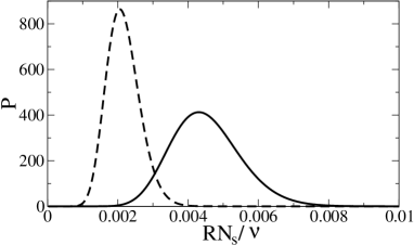
Figure 3: The probability distribution function $P$ for the total nucleation rate $RN_{s}$. It is obtained using Bayes’s theorem applied to $N_{A}=20$ measurements of the time $t$ at which the first nucleus appears. The true nucleation rates are $RN_{s}=3.623\times 10^{-3}\nu$ (solid curve) and $RN_{s}=1.575\times 10^{-3}\nu$ (dashed curve).

We have numerically generated sets of $N_{A}=20$ nucleation times for both systems and used both sets of values in Eq. (3). The two resulting probability distribution functions, $P(RN_{s}|\{t\})$, are plotted in Fig. 3. We used a prior of width $R_{0}=5\times 10^{-2}\nu$. Even with such a broad prior, 20 measurements are clearly enough to demonstrate that it is very likely that the two systems have different nucleation rates. Thus, the use of Bayes’s theorem in this way is an effective way of determining that the rate is varying from sample to sample, and so the rate is not self-averaging.

V Conclusion

Nucleation often occurs with the nucleus interacting with, and with a free energy strongly reduced by, impurities. This is called heterogeneous nucleation. Here, we have addressed the question: Under what conditions can chance variations from sample to sample in the impurities present, cause the nucleation rate to vary significantly from sample to sample? In the previous section we showed how Bayes’s theorem allows an efficient estimation of the nucleation rate in a sample and so allows variations in this rate to be detected. As the impurities are typically uncharacterised and uncontrolled we resorted to a statistical theory to model chance, i.e., random, variations in the impurities. The impurities were modelled by quenched disorder and we showed that the rate of nucleation has the same form as the partition function of Derrida’s Random Energy Model derrida80 . There is a regime where the nucleation rate in different samples prepared in the same way may be different, where it is non-self-averaging. This occurs when the width $w$ of the distribution of nucleation barriers is large. The crossover from this regime to the regime where the nucleation rate is very similar in different samples occurs at a width $w$ given by Eq. (10). The nucleation rate is very sensitive to disorder in the sense that it may be non-self-averaging even when other properties may still be self-averaging. This is in accord with experiment where nucleation is known to be highly sensitive to impurities perpezko84 . Our study of a specific model of nucleation at a disordered surface (section III) showed that, at least within this model, the origin of this sensitivity lies in the fact that the nucleus is quite large, it consists of not one but many molecules, and that the rate is proportional to the exponential of the free-energy barrier. Nucleation is important in a number of fields, for example, it is crucial for protein crystallisation durbin96 . The crystal phase of proteins is required for X-ray determination of their structure.

The method of direct observations of nucleation and applying Bayes’s theorem, is not the only way of estimating the effect of disorder on nucleation. An alternative way is to follow the fraction of the system that has undergone the phase transition as a function of time. The evolution over time $\tau$ of this fraction, which we denote by $X(\tau)$, is often described using the Kolmogorov-Johnson-Mehl-Avrami (KJMA) theory castro99 ; castro03 , according to which

$$X(\tau)=1-\exp(-A\tau^{m}),$$ (33)

where $A$ is a constant that depends on both the rate of nucleation and the rate of growth of the droplets/crystallites of the new phase. Equation (33) is sometimes referred to as Avrami’s law. If the nucleation rate is uniform throughout the system, the exponent $m=d+1$ with $d$ the dimensionality of space. The power of $d+1$ contains a power of $d$ due to the fact that if the growth front of the domains of the new phase is moving at a constant velocity $v$, then the volume of a domain scales as $(v\tau)^{d}$. The additional power of time comes from the fact that for uniform nucleation the number of domains increases linearly with time $\tau$. However, if nucleation is not uniform but occurs at just a few sites then nucleation may occur at early times at these sites, and then nucleation ceases as the sites with low free-energy barriers have been ‘used up’. Then the KJMA exponent $m$ equals $d$ not $d+1$. The nucleation rates $R$ calculated here are initial rates, when the rate $R$ is dominated by a few sites it will decrease as they are ‘used up’. Thus, as has been discussed by Castro and coworkers castro99 ; castro03 , disorder can result in deviations from a simple KJMA growth law with exponent $m=3$. See Refs. castro99 ; castro03 for calculations showing effective exponents between 2 and 3. We would expect that non-self-averaging systems, where nucleation occurs predominantly at one or a few sites, should exhibit an exponent near to $m=2$. It should be noted that they point out that $m$ alone is a not a particularly discriminating and that if the new phase forming is crystalline, then the grain size distribution provides more information.

Finally, Harrowell and Oxtoby harrowell93 have discussed the effects of the rapidly increasing relaxation time, essentially our $\nu^{-1}$, and heterogeneity present in a glass. Of course, glassy systems show non-self-averaging behaviour. Future work could study non-self-averaging behaviour of the nucleation rate in glasses.

It is a pleasure to acknowledge that this work has benefited greatly from discussions with J. Cuesta. This work was supported by The Wellcome Trust (069242).

References

- (1) P. G. Debenedetti, Metastable Liquids (Princeton University Press, Princeton, 1996).
- (2) V. G. Karpov, Phys. Rev. B 50, 9124 (1994).
- (3) V. G. Karpov and D. W. Oxtoby, Phys. Rev. B 54, 9734 (1996).
- (4) P. Harrowell and D. W. Oxtoby, Ceramic Trans. 30, 35 (1993).
- (5) M. Castro, F. Domínguez-Adame, A. Sánchez and T. Rodríguez, App. Phys. Lett. 75, 2205 (1999).
- (6) M. Castro, Phys. Rev. B 67, 035412 (2003).
- (7) V. G. Karpov, Phys. Rev. B 52, 15846 (1995).
- (8) D. W. Oxtoby, J. Phys.: Cond. Matt. 4 7627 (1992).
- (9) D. Kashchiev and G. M. van Rosmalen, Cryst. Res. Technol. 38, 555 (2003).
- (10) B. Derrida, Phys. Rev. Lett. 45, 79 (1980); Phys. Rev. B 24, 2613 (1981).
- (11) R. P. Sear, unpublished work.
- (12) D. Sornette, Critical Phenomena in Natural Sciences (Springer-Verlag, Berlin, 2000).
- (13) E. Gardner and B. Derrida, J. Phys. A 22, 1975 (1989).
- (14) S. D. Durbin and G. Feher, Ann. Rev. Phys. Chem. 47, 171 (1996).
- (15) J. H. Turnbull and R. E. Cech, J. App. Phys. 21, 804 (1950).
- (16) J. H. Perpezko, Mater. Sci. Eng. 65, 125 (1984).
- (17) D. J. C. MacKay, Information Theory, Inference, and Learning Algorithms (Cambridge University Press, Cambridge, 2003)
- (18) O. Galkin and P. G. Vekilov, J. Phys. Chem. 103, 10965 (1999).
- (19) P. G. Vekilov and O. Galkin, Coll. Surf. A 215, 125 (2003).