Andreev billiards

Abstract

This is a review of recent advances in our understanding of how Andreev reflection at a superconductor modifies the excitation spectrum of a quantum dot. The emphasis is on two-dimensional impurity-free structures in which the classical dynamics is chaotic. Such Andreev billiards differ in a fundamental way from their non-superconducting counterparts. Most notably, the difference between chaotic and integrable classical dynamics shows up already in the level density, instead of only in the level–level correlations. A chaotic billiard has a gap in the spectrum around the Fermi energy, while integrable billiards have a linearly vanishing density of states. The excitation gap $E_{\rm gap}$ corresponds to a time scale $\hbar/E_{\rm gap}$ which is classical ($\hbar$-independent, equal to the mean time $\tau_{\rm dwell}$ between Andreev reflections) if $\tau_{\rm dwell}$ is sufficiently large. There is a competing quantum time scale, the Ehrenfest time $\tau_{E}$, which depends logarithmically on $\hbar$. Two phenomenological theories provide a consistent description of the $\tau_{E}$-dependence of the gap, given qualitatively by $E_{\rm gap}\simeq\min(\hbar/\tau_{\rm dwell},\hbar/\tau_{E})$. The analytical predictions have been tested by computer simulations but not yet experimentally.

I Introduction

Forty years ago, Andreev discovered a peculiar property of superconducting mirrors And64 . As illustrated in Fig. 1, an electron that tries to enter a superconductor coming from the Fermi level of a normal metal is forced to retrace its path, as if time is reversed. Also the charge of the particle is reversed, since the negatively charged electron is converted into a positively charged hole. The velocity of a hole is opposite to its momentum, so the superconducting mirror conserves the momentum of the reflected particle. In contrast, reflection at an ordinary mirror (an insulator) conserves charge but not momentum. The unusual scattering process at the interface between a normal metal (N) and a superconductor (S) is called Andreev reflection.

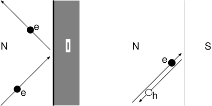
Figure 1: Normal reflection by an insulator (I) versus Andreev reflection by a superconductor (S) of an electron excitation in a normal metal (N) near the Fermi energy $E_{F}$. Normal reflection (left) conserves charge but does not conserve momentum. Andreev reflection (right) conserves momentum but does not conserve charge: The electron (e) is reflected as a hole (h) with the same momentum and opposite velocity. The missing charge of $2e$ is absorbed as a Cooper pair by the superconducting condensate. The electron-hole symmetry is exact at the Fermi level. If the electron is at a finite energy $E$ above $E_{F}$, then the hole is at an energy $E$ below $E_{F}$. The energy difference of $2E$ breaks the electron-hole symmetry. From Ref. Bee97 .

Andreev reflection is the key concept needed to understand the properties of nanostructures with NS interfaces Imr02 . Most of the research has concentrated on transport properties of open structures, see Refs. Bee97 ; Wee97 for reviews. There experiment and theory have reached a comparable level of maturity. In the present review we focus on spectral properties of closed structures, such as the quantum dot with superconducting contacts shown in Fig. 2. The theoretical understanding of these systems, gained from the combination of analytical theory and computer simulations, has reached the stage that a comprehensive review is called for — even though an experimental test of the theoretical predictions is still lacking.

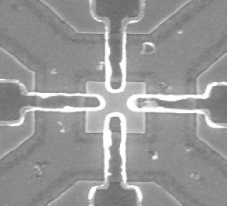
Figure 2: Quantum dot (central square of dimensions $500\,{\rm nm}\times 500\,{\rm nm}$) fabricated in a high-mobility InAs/AlSb heterostructure and contacted by four superconducting Nb electrodes. Device made by A. T. Filip, Groningen University (unpublished figure).

An impurity-free quantum dot in contact with a superconductor has been called an “Andreev billiard” Kos95 . The name is appropriate, and we will use it too, because it makes a connection with the literature on quantum chaos Gut90 ; Haa01 . A billiard (in the sense of a bounded two-dimensional region in which all scattering occurs at the boundaries) is the simplest system in which to search for quantum mechanical signatures of chaotic classical dynamics. That is the basic theme of the field of quantum chaos. By introducing a superconducting segment in the boundary of a billiard one has the possibility of unraveling the chaotic dynamics, so to say by making time flow backwards. Andreev billiards therefore reveal features of the chaotic dynamics that are obscured in their normal (non-superconducting) counterparts.

The presence of even the smallest superconducting segment suppresses the quantum mechanical level density at sufficiently low excitation energies. This suppression may take the form of an excitation gap, at an energy $E_{\rm gap}$ well below the gap $\Delta$ in the bulk superconductor (hence the name “minigap”). It may also take the form of a level density that vanishes smoothly (typically linearly) upon approaching the Fermi level, without an actual gap. The presence or absence of a gap is a quantum signature of chaos. That is a fundamental difference between normal billiards and Andreev billiards, since in a normal billiard the level density can not distinguish chaotic from integrable classical dynamics. (It depends only on the area of the billiard, not on its shape.)

A powerful technique to determine the spectrum of a chaotic system is random-matrix theory (RMT) Bee97 ; Meh91 ; Guh98 . Although the appearance of an excitation gap is a quantum mechanical effect, the corresponding time scale $\hbar/E_{\rm gap}$ as it follows from RMT is a classical (meaning $\hbar$-independent) quantity: It is the mean time $\tau_{\rm dwell}$ that an electron or hole excitation dwells in the billiard between two subsequent Andreev reflections. A major development of the last few years has been the discovery of a competing quantum mechanical time scale $\tau_{E}\propto|\ln\hbar|$. (The subscript E stands for Ehrenfest.) RMT breaks down if $\tau_{E}\gtrsim\tau_{\rm dwell}$ and a new theory is needed to determine the excitation gap in this regime. Two different phenomenological approaches have now reached a consistent description of the $\tau_{E}$-dependence of the gap, although some disagreement remains.

The plan of this review is as follows. The next four sections contain background material on Andreev reflection (Sec. II), on the minigap in NS junctions (Sec. III), on the scattering theory of Andreev billiards (Sec. IV), and on a stroboscopic model used in computer simulations (Sec. V). The regime of RMT (when $\tau_{E}\ll\tau_{\rm dwell}$) is described in Sec. VI and the quasiclassical regime (when $\tau_{E}\gg\tau_{\rm dwell}$) is described in Sec. VII. The crossover from $E_{\rm gap}\simeq\hbar/\tau_{\rm dwell}$ to $E_{\rm gap}\simeq\hbar/\tau_{E}$ is the topic of Sec. VIII. We conclude in Sec. IX.

II Andreev reflection

The quantum mechanical description of Andreev reflection starts from a pair of Schrödinger equations for electron and hole wave functions $u({\bf r})$ and $v({\bf r})$, coupled by the pair potential $\Delta({\bf r})$. These socalled Bogoliubov-De Gennes (BdG) equations DeG66 take the form

$${\cal H}_{\rm BG}\left(\begin{array}[]{c}u\\ v\end{array}\right)=E\left(\begin{array}[]{c}u\\ v\end{array}\right),$$ (5)

$${\cal H}_{\rm BG}=\left(\begin{array}[]{cc}H&{\Delta}({\bf r})\\ {\Delta}^{\ast}({\bf r})&-H^{\ast}\end{array}\right).$$ (8)

The Hamiltonian $H=({\bf p}+e{\bf A})^{2}/2m+V-E_{F}$ is the single-electron Hamiltonian in the field of a vector potential ${\bf A}({\bf r})$ and electrostatic potential $V({\bf r})$. The excitation energy $E$ is measured relative to the Fermi energy $E_{F}$. If $(u,v)$ is an eigenfunction with eigenvalue $E$, then $(-v^{\ast},u^{\ast})$ is also an eigenfunction, with eigenvalue $-E$. The complete set of eigenvalues thus lies symmetrically around zero. The quasiparticle excitation spectrum consists of all positive $E$.

In a uniform system with $\Delta({\bf r})\equiv\Delta$, ${\bf A}({\bf r})\equiv 0$, $V({\bf r})\equiv 0$, the solution of the BdG equations is

$$E = \left[(\hbar^{2}k^{2}/2m-E_{F})^{2}+\Delta^{2}\right]^{1/2},$$ (9)

$$u({\bf r}) = (2E)^{-1/2}\left(E+\hbar^{2}k^{2}/2m-E_{F}\right)^{1/2}e^{i{\bf k}\cdot{\bf r}},$$ (10)

$$v({\bf r}) = (2E)^{-1/2}\left(E-\hbar^{2}k^{2}/2m+E_{F}\right)^{1/2}e^{i{\bf k}\cdot{\bf r}}.$$ (11)

The excitation spectrum is continuous, with excitation gap $\Delta$. The eigenfunctions $(u,v)$ are plane waves characterized by a wavevector ${\bf k}$. The coefficients of the plane waves are the two coherence factors of the BCS (Bardeen-Cooper-Schrieffer) theory.

At an interface between a normal metal and a superconductor the pairing interaction drops to zero over atomic distances at the normal side. (We assume non-interacting electrons in the normal region.) Therefore, $\Delta({\bf r})\equiv 0$ in the normal region. At the superconducting side of the NS interface, $\Delta({\bf r})$ recovers its bulk value $\Delta$ only at some distance from the interface. This suppression of $\Delta({\bf r})$ is neglected in the step-function model

$$\Delta({\bf r})=\left\{\begin{array}[]{ll}\Delta&\;{\rm if}\;{\bf r}\in S,\\ 0&\;{\rm if}\;{\bf r}\in N.\end{array}\right.$$ (14)

The step-function pair potential is also referred to in the literature as a “rigid boundary condition” Lik79 . It greatly simplifies the analysis of the problem without changing the results in any qualitative way.

Since we will only be considering a single superconductor, the phase of the superconducting order parameter is irrelevant and we may take $\Delta$ real. (See Ref. Bee92b for a tutorial introduction to mesoscopic Josephson junctions, such as a quantum dot connected to two superconductors.)

III Minigap in NS junctions

The presence of a normal metal interface changes the excitation spectrum (proximity effect). The continuous spectrum above the bulk gap $\Delta$ differs from the BCS form (10) and in addition there may appear discrete energy levels $E_{n}<\Delta$.

The wave function of the lowest level contains electron and hole components $u_{0},v_{0}$ of equal magnitude, mixed by Andreev reflection. The mean time $\tau_{\rm dwell}$ between Andreev reflections (corresponding to the mean life time of an electron or hole excitation) sets the scale $E_{0}\equiv E_{\rm gap}\simeq\hbar/\tau_{\rm dwell}$ for the energy of this lowest level McM68 . This “minigap” is smaller than the bulk gap by a factor $\xi_{0}/v_{F}\tau_{\rm dwell}$, with $\xi_{0}=\hbar v_{F}/\Delta$ the superconducting coherence length and $v_{F}$ the Fermi velocity. The energy $\hbar/\tau_{\rm dwell}$ is called the Thouless energy $E_{T}$, because of the role it plays in Thouless’s theory of localization Imr02 .

The simplest NS junction, which can be analyzed exactly DeG63 , consists of an impurity-free normal metal layer (thickness $d$) on top of a bulk superconductor. Because of translational invariance parallel to the NS interface, the parallel component $p_{\parallel}$ of the momentum is a good quantum number. The lowest excitation energy

$$E_{0}(p_{\parallel})=\frac{\pi\hbar}{2T(p_{\parallel})},\;\;T(p_{\parallel})=\frac{2md}{(p_{F}^{2}-p_{\parallel}^{2})^{1/2}},$$ (15)

is the reciprocal of the time $T(p_{\parallel})$ between two subsequent Andreev reflections. This time diverges when $p_{\parallel}$ approaches the Fermi momentum $p_{F}=\hbar k_{F}=\sqrt{2mE_{F}}$, so $E_{0}$ can come microscopically close to zero. The lower limit $E_{0}\gtrsim\hbar^{2}/md^{2}$ is set by the quantization of the momentum perpendicular to the layer.

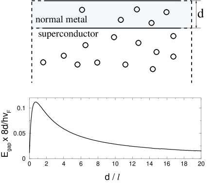
Figure 3: Excitation gap $E_{\rm gap}$ of a disordered NS junction, as a function of the ratio of the thickness $d$ of the normal metal layer and the mean free path $l$. The curve in the bottom panel is calculated from the disorder-averaged Green function (for $\xi_{0}\ll d,l$). The top panel illustrates the geometry. The normal metal layer has a specularly reflecting upper surface and an ideally transmitting lower surface. Adapted from Ref. Pil00 .

Impurities in the normal metal layer (with mean free path $l$) prevent the time between Andreev reflections to grow much larger than $\tau_{\rm dwell}\simeq\max(l/v_{F},d^{2}/v_{F}l)$. The excitation gap Gol88 ; Bel96 ; Pil00

$$E_{\rm gap}\simeq\hbar/\tau_{\rm dwell}\simeq(\hbar v_{F}l/d^{2})\min(1,d^{2}/l^{2})$$ (16)

is now a factor $k_{F}l\min(1,d^{2}/l^{2})$ larger than in the absence of impurities. A precise calculation using disorder-averaged Green functions (reviewed in Ref. Bel99 ) gives the curve shown in Fig. 3. The two asymptotes are Pil00

$$E_{\rm gap}=\left\{\begin{array}[]{cc}0.43\,\hbar v_{F}/l,&{\rm if}\;\;d/l\ll 1,\\ 0.78\,\hbar D/d^{2},&{\rm if}\;\;d/l\gg 1,\end{array}\right.$$ (17)

with $D=v_{F}l/3$ the diffusion constant in the normal metal.

The minigap in a ballistic quantum dot (Andreev billiard) differs from that in a disordered NS junction in two qualitative ways:

1. The opening of an excitation gap depends on the shape of the boundary, rather than on the degree of disorder Mel96 . A chaotic billiard has a gap at the Thouless energy $E_{T}\simeq\hbar/\tau_{\rm dwell}$, like a disordered NS junction. An integrable billiard has a linearly vanishing density of states, like a ballistic NS junction.

2. In a chaotic billiard a new time scale appears, the Ehrenfest time $\tau_{E}$, which competes with $\tau_{\rm dwell}$ in setting the scale for the excitation gap Lod98 . While $\tau_{\rm dwell}$ is a classical $\hbar$-independent time scale, $\tau_{E}\propto|\ln\hbar|$ has a quantum mechanical origin.

Because one can not perform a disorder average in Andreev billiards, the Green function formulation is less useful than in disordered NS junctions. Instead, we will make extensive use of the scattering matrix formulation, explained in the next section.

IV Scattering formulation

In the step-function model (14) the excitation spectrum of the coupled electron-hole quasiparticles can be expressed entirely in terms of the scattering matrix of normal electrons Bee91 .

The scattering geometry is illustrated in Fig. 4. It consists of a finite normal-metal region N adjacent to a semi-infinite superconducting region S. The metal region represents the Andreev billiard. To obtain a well-defined scattering problem we insert an ideal (impurity-free) normal lead between N and S. We assume that the only scattering in the superconductor consists of Andreev reflection at the NS interface (no disorder in S). The superconductor may then also be represented by an ideal lead. We choose a coordinate system so that the normal and superconducting leads lie along the $x$-axis, with the interface at $x=0$.

Figure 4: Normal metal (N) containing an Andreev billiard, coupled to a superconductor (S) by an ideal lead. The dashed line represents the NS interface. Scattering states $c^{\rm in}=(c_{\rm e}^{+},c_{\rm h}^{-})$ and $c^{\rm out}=(c_{\rm e}^{-},c_{\rm h}^{+})$ are indicated schematically.

We first construct a basis for the scattering matrix. In the normal lead N the eigenfunctions of the BdG equation (5) can be written in the form

$$\Psi_{n,{\rm e}}^{\pm}({\rm N})={\left(\begin{array}[]{c}1\\ 0\end{array}\right)}\frac{1}{\sqrt{k_{n}^{\rm e}}}\,\Phi_{n}(y,z)\exp(\pm{\rm i}k_{n}^{\rm e}x),$$ (18c)

$$\Psi_{n,{\rm h}}^{\pm}({\rm N})={\left(\begin{array}[]{c}0\\ 1\end{array}\right)}\frac{1}{\sqrt{k_{n}^{\rm h}}}\,\Phi_{n}(y,z)\exp(\pm{\rm i}k_{n}^{\rm h}x),$$ (18f)

where the wavenumbers $k_{n}^{\rm e}$ and $k_{n}^{\rm h}$ are given by

$$k_{n}^{\rm e,h}=\frac{\sqrt{2m}}{\hbar}(E_{F}-E_{n}+\sigma^{\rm e,h}E)^{1/2},$$ (19)

and we have defined $\sigma^{\rm e}\equiv 1$, $\sigma^{\rm h}\equiv-1$. The labels e and h indicate the electron or hole character of the wave function. The index $n$ labels the modes, $\Phi_{n}(y,z)$ is the transverse wave function of the $n$-th mode, and $E_{n}$ its threshold energy:

$$[(p_{y}^{2}+p_{z}^{2})/2m+V(y,z)]\Phi_{n}(y,z)=E_{n}\Phi_{n}(y,z).$$ (20)

The eigenfunction $\Phi_{n}$ is normalized to unity, $\int\!dy\int\!dz\,|\Phi_{n}|^{2}=1$.

In the superconducting lead S the eigenfunctions are

$$\Psi_{n,{\rm e}}^{\pm}({\rm S}) = {\left(\begin{array}[]{c}{\rm e}^{{\rm i}\eta^{\rm e}/2}\\ {\rm e}^{-{\rm i}\eta^{\rm e}/2}\end{array}\right)}\frac{1}{\sqrt{2q_{n}^{\rm e}}}(E^{2}/\Delta^{2}-1)^{-1/4}$$ (21d)

$$\mbox{}\times\Phi_{n}(y,z)\exp(\pm{\rm i}q_{n}^{\rm e}x),$$

$$\Psi_{n,{\rm h}}^{\pm}({\rm S}) = {\left(\begin{array}[]{c}{\rm e}^{{\rm i}\eta^{\rm h}/2}\\ {\rm e}^{-{\rm i}\eta^{\rm h}/2}\end{array}\right)}\frac{1}{\sqrt{2q_{n}^{\rm h}}}(E^{2}/\Delta^{2}-1)^{-1/4}$$ (21h)

$$\mbox{}\times\Phi_{n}(y,z)\exp(\pm{\rm i}q_{n}^{\rm h}x).$$

We have defined

$$q_{n}^{\rm e,h} = \frac{\sqrt{2m}}{\hbar}[E_{F}-E_{n}+\sigma^{\rm e,h}(E^{2}-\Delta^{2})^{1/2}]^{1/2},$$ (22)

$$\eta^{\rm e,h} = \sigma^{\rm e,h}\arccos(E/\Delta).$$ (23)

The wave functions (18) and (21) have been normalized to carry the same amount of quasiparticle current, because we want to use them as the basis for a unitary scattering matrix. The direction of the velocity is the same as the wave vector for the electron and opposite for the hole.

A wave incident on the Andreev billiard is described in the basis (18) by a vector of coefficients

$$c^{\rm in}=(c_{\rm e}^{+},c_{\rm h}^{-}),$$ (24)

as shown schematically in Fig. 4. (The mode index $n$ has been suppressed for simplicity of notation.) The reflected wave has vector of coefficients

$$c^{\rm out}=(c_{\rm e}^{-},c_{\rm h}^{+}).$$ (25)

The scattering matrix $S_{\rm N}$ of the normal region relates these two vectors, $c_{\rm N}^{\rm out}=S_{\rm N}c_{\rm N}^{\rm in}$. Because the normal region does not couple electrons and holes, this matrix has the block-diagonal form

$$S_{\rm N}(E)={\left(\begin{array}[]{cc}S(E)&0\\ \!0&S(-E)^{\ast}\end{array}\right)}.$$ (28)

Here $S(E)$ is the unitary scattering matrix associated with the single-electron Hamiltonian $H$. It is an $N\times N$ matrix, with $N(E)$ the number of propagating modes at energy $E$. The dimension of $S_{\rm N}(E)$ is $N(E)+N(-E)$.

For energies $0<E<\Delta$ there are no propagating modes in the superconducting lead S. Restricting ourselves to that energy range, we can define a scattering matrix $S_{\rm A}$ for Andreev reflection at the NS interface by $c^{\rm in}=S_{\rm A}c^{\rm out}$. The elements of $S_{\rm A}$ are obtained by matching the wave function (18) at $x=0$ to the decaying wave function (21). Since $\Delta\ll E_{F}$ one may ignore normal reflections at the NS interface and neglect the difference between $N(E)$ and $N(-E)$. This is known as the Andreev approximation And64 . The result is

$$S_{\rm A}(E)={\left(\begin{array}[]{cc}0&\alpha(E)\\ \alpha(E)&0\end{array}\right)},$$ (31)

$$\alpha(E)=e^{-i\arccos(E/\Delta)}=\frac{E}{\Delta}-i\sqrt{1-\frac{E^{2}}{\Delta^{2}}}.$$ (32)

Andreev reflection transforms an electron mode into a hole mode, without change of mode index. The transformation is accompanied by a phase shift $-\arccos(E/\Delta)$ due to the penetration of the wave function into the superconductor.

We are now ready to relate the excitation spectrum of the Andreev billiard to the scattering matrix of the normal region. We restrict ourselves to the discrete spectrum (see Ref. Bee91 for the continuous spectrum). The condition $c_{\rm in}=S_{\rm A}S_{\rm N}c_{\rm in}$ for a bound state implies ${\rm Det}\,(1-S_{\rm A}S_{\rm N})=0$. Using Eqs. (28), (31), and the identity

$${\rm Det}\,{\left(\begin{array}[]{cc}a&b\\ c&d\end{array}\right)}={\rm Det}\,(ad-aca^{-1}b)$$ (35)

one obtains the equation Bee91

$${\rm Det}\,\left[1-\alpha(E)^{2}S(E)S(-E)^{\ast}\right]=0.$$ (36)

The roots $E_{p}$ of this determinantal equation constitute the discrete spectrum of the Andreev billiard.

V Stroboscopic model

Although the phase space of the Andreev billiard is four-dimensional, like for any billiard it can be reduced to two dimensions on a Poincaré surface of section Gut90 ; Haa01 . This amounts to a stroboscopic description of the classical dynamics, because the position and momentum are only recorded when the particle crosses the surface of section. Quantum mechanically, the stroboscopic evolution of the wave function is described by a compact unitary map rather than by a noncompact Hermitian operator Bog92 ; Pra03 . What one loses by the stroboscopic description is information on time scales below the time of flight across the billiard. What one gains is an enormous increase in computational efficiency.

A stroboscopic model of an Andreev billiard was constructed by Jacquod et al. Jac03 , building on an existing model for open normal billiards called the open kicked rotator Oss02 . The Andreev kicked rotator possesses the same phenomenology as the Andreev billiard, but is much more tractable numerically. In this subsection we discuss how it is formulated. Some results obtained by this numerical method will be compared in subsequent sections with results obtained by analytical means.

A compact unitary map is represented in quantum mechanics by the Floquet operator $F$, which gives the stroboscopic time evolution $u(p\tau_{0})=F^{p}u(0)$ of an initial wave function $u(0)$. (We set the stroboscopic period $\tau_{0}=1$ in most equations.) The unitary $M\times M$ matrix $F$ has eigenvalues $\exp(-i\varepsilon_{m})$, with the quasi-energies $\varepsilon_{m}\in(-\pi,\pi)$ (measured in units of $\hbar/\tau_{0}$). This describes the electron excitations above the Fermi level. Hole excitations below the Fermi level have Floquet operator $F^{\ast}$ and wave function $v(p)=(F^{\ast})^{p}v(0)$. The mean level spacing of electrons and holes separately is $\delta=2\pi/M$.

An electron is converted into a hole by Andreev reflection at the NS interface, with phase shift $-i$ for $\varepsilon\ll\tau_{0}\Delta/\hbar$ [cf. Eq. (32)]. In the stroboscopic description one assumes that Andreev reflection occurs only at times which are multiples of $\tau_{0}$. The $N\times M$ matrix $P$ projects onto the NS interface. Its elements are $P_{nm}=1$ if $m=n\in\{n_{1},n_{2},\ldots n_{N}\}$ and $P_{nm}=0$ otherwise. The dwell time of a quasiparticle excitation in the normal metal is $\tau_{\rm dwell}=M/N$, equal to the mean time between Andreev reflections.

Putting all this together one constructs the quantum Andreev map from the matrix product

$${\cal F}={\cal P}\left(\begin{array}[]{cc}F&0\\ 0&F^{\ast}\end{array}\right),\;\;{\cal P}=\left(\begin{array}[]{cc}1-P^{\rm T}P&-iP^{\rm T}P\\ -iP^{\rm T}P&1-P^{\rm T}P\end{array}\right).$$ (37)

(The superscript “T” indicates the transpose of a matrix.) The particle-hole wave function $\Psi=(u,v)$ evolves in time as $\Psi(p)={\cal F}^{p}\Psi(0)$. The Floquet operator can be symmetrized (without changing its eigenvalues) by the unitary transformation ${\cal F}\rightarrow{\cal P}^{-1/2}{\cal F}{\cal P}^{1/2}$, with

$${{\cal P}^{1/2}=\left(\begin{array}[]{cc}1-(1-{\textstyle\frac{1}{2}}\sqrt{2})P^{\rm T}P&-i{\textstyle\frac{1}{2}}\sqrt{2}P^{\rm T}P\\ -i{\textstyle\frac{1}{2}}\sqrt{2}P^{\rm T}P&1-(1-{\textstyle\frac{1}{2}}\sqrt{2})P^{\rm T}P\end{array}\right).}$$ (38)

The quantization condition ${\rm det}({\cal F}-e^{-i\varepsilon})=0$ can be written equivalently as Jac03

$${\rm Det}\,[1+S(\varepsilon)S(-\varepsilon)^{\ast}]=0,$$ (39)

in terms of the $N\times N$ scattering matrix Oss02 ; Fyo00

$$S(\varepsilon)=P[e^{-i\varepsilon}-F(1-P^{\rm T}P)]^{-1}FP^{\rm T}.$$ (40)

Eq. (39) for the Andreev map has the same form as Eq. (36) for the Andreev billiard (with $\alpha\rightarrow-i$). In particular, both equations have roots that lie symmetrically around zero.

A specific realization of the Andreev map is the Andreev kicked rotator. (See Ref. Oss04 for a different realization, based on the kicked Harper model.) The normal kicked rotator has Floquet operator Izr90

$$F = \exp\left(i\frac{\hbar\tau_{0}}{4I_{0}}\frac{\partial^{2}}{\partial\theta^{2}}\right)\exp\left(-i\frac{KI_{0}}{\hbar\tau_{0}}\cos\theta\right)$$ (41)

$$\mbox{}\times\exp\left(i\frac{\hbar\tau_{0}}{4I_{0}}\frac{\partial^{2}}{\partial\theta^{2}}\right).$$

It describes a particle that moves freely along the unit circle $(\cos\theta,\sin\theta)$ with moment of inertia $I_{0}$ for half a period $\tau_{0}$, is then kicked with a strength $K\cos\theta$, and proceeds freely for another half period. Upon increasing $K$ the classical dynamics varies from fully integrable ($K=0$) to fully chaotic [$K\gtrsim 7$, with Lyapunov exponent $\alpha\approx\ln(K/2)$]. For $K<7$ stable and unstable motion coexist (mixed phase space). If needed, a magnetic field can be introduced into the model as described in Ref. Two04 .

The transition from classical to quantum behavior is governed by the effective Planck constant $h_{\rm eff}\equiv\hbar\tau_{0}/2\pi I_{0}$. For $1/h_{\rm eff}\equiv M$ an even integer, $F$ can be represented by an $M\times M$ unitary symmetric matrix. The angular coordinate and momentum eigenvalues are $\theta_{m}=2\pi m/M$ and $p_{m}=\hbar m$, with $m=1,2,\ldots M$, so phase space has the topology of a torus. The NS interface is an annulus around the torus, either in the $\theta$-direction or in the $p$-direction. (The two configurations give equivalent results.) The construction (37) produces a $2M\times 2M$ Floquet operator ${\cal F}$, which can be diagonalized efficiently in ${\cal O}(M^{2}\ln M)$ operations [rather than ${\cal O}(M^{3})$] by combining the Lanczos technique with the fast-Fourier-transform algorithm Ket99 .

VI Random-matrix theory

An ensemble of isolated chaotic billiards, constructed by varying the shape at constant area, corresponds to an ensemble of Hamiltonians $H$ with a particular distribution function $P(H)$. It is convenient to think of the Hamiltonian as a random $M\times M$ Hermitian matrix, eventually sending $M$ to infinity. The basic postulate of random-matrix theory (RMT) Meh91 is that the distribution is invariant under the unitary transformation $H\rightarrow UHU^{\dagger}$, with $U$ an arbitrary unitary matrix. This implies a distribution of the form

$$P(H)\propto\exp[-{\rm Tr}\,V(H)].$$ (42)

If $V(H)\propto H^{2}$, the ensemble is called Gaussian. This choice simplifies some of the calculations but is not essential, because the spectral correlations become largely independent of $V$ in the limit $M\rightarrow\infty$. More generally, the ensemble of the form (42) is called the Wigner-Dyson ensemble, after the founding fathers of RMT.

By computing the Jacobian from the space of matrix elements to the space of eigenvalues $E_{n}$ ($n=1,2,\ldots M$), one obtains the eigenvalue probability distribution Meh91

$$P(\{E_{n}\})\propto\prod_{i<j}|E_{i}-E_{j}|^{\beta}\prod_{k}e^{-V(E_{k})}.$$ (43)

The symmetry index $\beta$ counts the number of degrees of freedom in the matrix elements. These are real ($\beta=1$) in the presence of time-reversal symmetry or complex ($\beta=2$) in its absence. (A third possibility, $\beta=4$, applies to time-reversally symmetric systems with strong spin-orbit scattering, which we will not consider here.) Since the unitary transformation $H\rightarrow UHU^{\dagger}$ requires an orthogonal $U$ to keep a real Hamiltonian, one speaks of the Gaussian orthogonal ensemble (GOE) when $\beta=1$. The name Gaussian unitary ensemble (GUE) refers to $\beta=2$.

There is overwhelming numerical evidence that chaotic billiards are well described by the Wigner-Dyson ensemble Haa01 . (This is known as the Bohigas-Giannoni-Schmit conjecture Boh84 .) A complete theoretical justification is still lacking, but much progress has been made in that direction Mul04 . In this section we will take Eq. (42) for the ensemble of isolated billiards as our starting point and deduce what properties it implies for the ensemble of Andreev billiards.

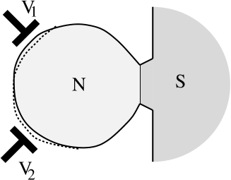
Figure 5: A quantum dot (N) connected to a superconductor (S). The voltages on the gates $V_{1}$ and $V_{2}$ change the shape of the dot. Different values of the applied voltages create different samples within the same ensemble. From Ref. Vav01 .

The isolated billiard becomes an Andreev billiard when it is connected by a point contact to a superconductor, cf. Fig. 5. In the isolated billiard RMT breaks down on energy scales greater than $\hbar/\tau_{\rm erg}$, with the ergodic time $\tau_{\rm erg}\simeq A^{1/2}/v_{F}$ set by the time of flight across the billiard (of area $A$, at Fermi velocity $v_{F}$). On larger energy scales, hence on shorter time scales, non-chaotic dynamics appears which is beyond RMT. The superconductor affects the billiard in an energy range around the Fermi level that is set by the Thouless energy $E_{T}\simeq\hbar/\tau_{\rm dwell}$. (We assume that $E_{T}$ is less than the gap $\Delta$ in the bulk superconductor.) In this context the dwell time $\tau_{\rm dwell}$ is the mean time between Andreev reflections (being the life time of an electron or hole quasiparticle). The condition $\tau_{\rm erg}\ll\tau_{\rm dwell}$ of weak coupling is therefore sufficient to be able to apply RMT to the entire relevant energy range.

VI.1 Effective Hamiltonian

The excitation energies $E_{p}$ of the Andreev billiard in the discrete part of the spectrum are the solutions of the determinantal equation (36), given in terms of the scattering matrix $S(E)$ in the normal state (i.e. when the superconductor is replaced by a normal metal). This equation can alternatively be written in terms of the Hamiltonian $H$ of the isolated billiard and the $M\times N$ coupling matrix $W$ that describes the $N$-mode point contact. The relation between $S$ and $H,W$ is Guh98 ; Bee97

$$S(E)=1-2\pi iW^{T}(E-H+i\pi WW^{T})^{-1}W.$$ (44)

The $N\times N$ matrix $W^{T}W$ has eigenvalues $w_{n}$ given by

$$w_{n}=\frac{M\delta}{\pi^{2}\Gamma_{n}}\left(2-\Gamma_{n}-2\sqrt{1-\Gamma_{n}}\right),$$ (45)

where $\delta$ is the mean level spacing in the isolated billiard and $\Gamma_{n}\in[0,1]$ is the transmission probability of mode $n=1,2,\ldots N$ in the point contact. For a ballistic contact, $\Gamma_{n}=1$, while $\Gamma_{n}\ll 1$ for a tunneling contact. Both the number of modes $N$ and the level spacing $\delta$ refer to a single spin direction.

Substituting Eq. (44) into Eq. (36), one arrives at an alternative determinantal equation for the discrete spectrum Bro97a :

$${\rm Det}\,[E-{\cal H}+{\cal W}(E)]=0,$$ (46)

$${\cal H}=\left(\begin{array}[]{cc}H&0\\ 0&-H^{\ast}\end{array}\right),$$ (49)

$${\cal W}(E)=\frac{\pi}{\sqrt{\Delta^{2}-E^{2}}}\left(\begin{array}[]{cc}EWW^{T}&\Delta WW^{T}\\ \Delta WW^{T}&EWW^{T}\end{array}\right).$$ (52)

The density of states follows from

$$\rho(E)=-\frac{1}{\pi}{\rm Im}\,{\rm Tr}\,(1+d{\cal W}/dE)(E+i0^{+}-{\cal H}+{\cal W})^{-1}.$$ (53)

In the relevant energy range $E\lesssim E_{T}\ll\Delta$ the matrix ${\cal W}(E)$ becomes energy independent. The excitation energies can then be obtained as the eigenvalues of the effective Hamiltonian Fra96

$${\cal H}_{\rm eff}=\left(\begin{array}[]{cc}H&-\pi WW^{T}\\ -\pi WW^{T}&-H^{\ast}\end{array}\right).$$ (54)

The effective Hamiltonian ${\cal H}_{\rm eff}$ should not be confused with the Bogoliubov-de Gennes Hamiltonian ${\cal H}_{\rm BG}$, which contains the superconducting order parameter in the off-diagonal blocks [cf. Eq. (8)]. The Hamiltonian ${\cal H}_{\rm BG}$ determines the entire excitation spectrum (both the discrete part below $\Delta$ and the continuous part above $\Delta$), while the effective Hamiltonian ${\cal H}_{\rm eff}$ determines only the low-lying excitations $E_{p}\ll\Delta$.

The Hermitian matrix ${\cal H}_{\rm eff}$ (like ${\cal H}_{\rm BG}$) is antisymmetric under the combined operation of charge conjugation (${\cal C}$) and time inversion (${\cal T}$) Alt96 :

$${\cal H}_{\rm eff}=-\sigma_{y}{\cal H}_{\rm eff}^{T}\sigma_{y},\;\;\sigma_{y}=\left(\begin{array}[]{cc}0&-i\\ i&0\\ \end{array}\right).$$ (55)

(An $M\times M$ unit matrix in each of the four blocks of $\sigma_{y}$ is implicit.) The ${\cal CT}$-antisymmetry ensures that the eigenvalues lie symmetrically around $E=0$. Only the positive eigenvalues are retained in the excitation spectrum, but the presence of the negative eigenvalues is felt as a level repulsion near $E=0$.

VI.2 Excitation gap

In zero magnetic field the suppression of the density of states $\rho(E)$ around $E=0$ extends over an energy range $E_{T}$ that may contain many level spacings $\delta$ of the isolated billiard. The ratio $g\simeq E_{T}/\delta$ is the conductance of the point contact in units of the conductance quantum $e^{2}/h$. For $g\gg 1$ the excitation gap $E_{\rm gap}\simeq g\delta$ is a mesoscopic quantity, because it is intermediate between the microscopic energy scale $\delta$ and the macroscopic energy scale $\Delta$. One can use perturbation theory in the small parameter $1/g$ to calculate $\rho(E)$. The analysis presented here follows the RMT of Melsen et al. Mel96 . An alternative derivation Vav03 , using the disorder-averaged Green function, is discussed in the next sub-section.

In the presence of time-reversal symmetry the Hamiltonian $H$ of the isolated billiard is a real symmetric matrix. The appropriate RMT ensemble is the GOE, with distribution Meh91

$$P(H)\propto\exp\left(-\frac{\pi^{2}}{4M\delta^{2}}{\rm Tr}\,H^{2}\right).$$ (56)

The ensemble average $\langle\cdots\rangle$ is an average over $H$ in the GOE at fixed coupling matrix $W$. Because of the block structure of ${\cal H}_{\rm eff}$, the ensemble averaged Green function ${\cal G}(E)=\langle(E-{\cal H}_{\rm eff})^{-1}\rangle$ consists of four $M\times M$ blocks ${\cal G}_{11}$, ${\cal G}_{12}$, ${\cal G}_{21}$, ${\cal G}_{22}$. By taking the trace of each block separately, one arrives at a $2\times 2$ matrix Green function

$$G=\left(\begin{array}[]{cc}G_{11}&G_{12}\\ G_{21}&G_{22}\end{array}\right)=\frac{\delta}{\pi}\left(\begin{array}[]{cc}{\rm Tr}\,{\cal G}_{11}&{\rm Tr}\,{\cal G}_{12}\\ {\rm Tr}\,{\cal G}_{21}&{\rm Tr}\,{\cal G}_{22}\end{array}\right).$$ (57)

(The factor $\delta/\pi$ is inserted for later convenience.)

The average over the distribution (56) can be done diagrammatically Pan81 ; Brez94 . To leading order in $1/M$ and for $E\gg\delta$ only simple (planar) diagrams need to be considered. Resummation of these diagrams leads to the selfconsistency equation Mel96 ; Bro97a

$${\cal G}=[E+{\cal W}-(M\delta/\pi)\sigma_{z}G\sigma_{z}]^{-1},\;\;\sigma_{z}=\left(\begin{array}[]{cc}1&0\\ 0&-1\\ \end{array}\right).$$ (58)

This is a matrix-generalization of Pastur’s equation in the RMT of normal systems Pas72 .

The matrices in Eq. (58) have four $M\times M$ blocks. By taking the trace of each block one obtains an equation for a $4\times 4$ matrix,

$$G=\frac{1}{M}\sum_{m=1}^{M}\left(\begin{array}[]{cc}\pi E/M\delta-G_{11}&\tilde{w}_{m}+G_{12}\\ \tilde{w}_{m}+G_{21}&\pi E/M\delta-G_{22}\end{array}\right)^{-1},$$ (61)

$$\tilde{w}_{m}=\left\{\begin{array}[]{cc}\pi^{2}w_{m}/M\delta&{\rm if}\;\;m=1,2,\ldots N,\\ 0&{\rm if}\;\;m=N+1,\ldots M.\end{array}\right.$$ (64)

Since $G_{22}=G_{11}$ and $G_{21}=G_{12}$ there are two unknown functions to determine. For $M\gg N$ these satisfy

$$G_{12}^{2}=1+G_{11}^{2},$$ (65a)

$$\frac{2\pi E}{\delta}G_{12}=G_{11}\sum_{n=1}^{N}(-G_{12}+1-2/\Gamma_{n})^{-1},$$ (65b)

where we have used the relation (45) between the parameters $w_{n}$ and the transmission probabilities $\Gamma_{n}$. Eq. (65) has multiple solutions. The physical solution satisfies $\lim_{E\rightarrow\infty}\langle\rho(E)\rangle=2/\delta$, when substituted into

$$\langle\rho(E)\rangle=-(2/\delta)\,{\rm Im}\,G_{11}(E).$$ (66)

Figure 6: Ensemble averaged density of states of a chaotic billiard coupled by a point contact to a superconductor, for several values of the transmission probability through the point contact. The energy is in units of the Thouless energy $E_{T}=N\Gamma\delta/4\pi$. The solid curves are computed from Eqs. (65) and (66), for mode-independent transmission probabilities $\Gamma=1$, $0.5$, $0.25$, $0.1$. The dashed curve is the asymptotic result (73) for $\Gamma\ll 1$. Adapted from Ref. Mel96 . (The definition of $\delta$ used in that paper differs from the one used here by a factor of two.)

In Fig. 6 we plot the density of states in the mode-independent case $\Gamma_{n}\equiv\Gamma$, for several vaues of $\Gamma$. It vanishes as a square root near the excitation gap. The value of $E_{\rm gap}$ can be determined directly by solving Eq. (65) jointly with $dE/dG_{11}=0$. The result is

$$\frac{k^{6}-k^{4}}{(1-k)^{6}}x^{6}-\frac{3k^{4}-20k^{2}+16}{(1-k)^{4}}x^{4}+\frac{3k^{2}+8}{(1-k)^{2}}x^{2}=1,$$

$$x=E_{\rm gap}/E_{T},\;k=1-2/\Gamma,\;E_{T}=N\Gamma\delta/4\pi.$$ (67)

For later use we parametrize the square-root dependence near the gap as

$$\langle\rho(E)\rangle\rightarrow\frac{1}{\pi}\sqrt{\frac{E-E_{\rm gap}}{\Delta^{3}_{\rm gap}}},\;\;E\rightarrow E_{\rm gap}.$$ (68)

When $E\gg E_{\rm gap}$ the density of states approaches the value $2/\delta$ from above, twice the value in the isolated billiard. The doubling of the density of states occurs because electron and hole excitations are combined in the excitation spectrum of the Andreev billiard, while in an isolated billiard electron and hole excitations are considered separately.

A rather simple closed-form expression for $\langle\rho(E)\rangle$ exists in two limiting cases Mel96 . In the case $\Gamma=1$ of a ballistic point contact one has

$$\langle\rho(E)\rangle=\frac{E_{T}\sqrt{3}}{3E\delta}[Q_{+}(E/E_{T})-Q_{-}(E/E_{T})],$$ (69)

$$Q_{\pm}(x)=\left[8-36x^{2}\pm 3x\sqrt{3x^{4}+132x^{2}-48}\right]^{1/3},$$ (70)

$$E>E_{\rm gap}=2\gamma^{5/2}E_{T}=0.60\,E_{T}=\frac{0.30\,\hbar}{\tau_{\rm dwell}}=0.048\,N\delta,$$

(71)

where $\gamma=\frac{1}{2}(\sqrt{5}-1)$ is the golden number. In this case the parameter $\Delta_{\rm gap}$ in Eq. (68) is given by

$$\Delta_{\rm gap}=[(5-2\sqrt{5})\delta^{2}E_{\rm gap}/8\pi^{2}]^{1/3}=0.068\,N^{1/3}\delta.$$ (72)

In the opposite tunneling limit $\Gamma\ll 1$ one finds

$$\langle\rho(E)\rangle=\frac{2E}{\delta}({E^{2}-E_{T}^{2}})^{-1/2},\;E>E_{\rm gap}=E_{T}.$$ (73)

In this limit the density of states of the Andreev billiard has the same form as in the BCS theory for a bulk superconductor Tin95 , with a reduced value of the gap (“minigap”). The inverse square-root singularity at the gap is cut off for any finite $\Gamma$, cf. Fig. 6.

VI.3 Effect of impurity scattering

Impurity scattering in a chaotic Andreev billiard reduces the magnitude of the excitation gap by increasing the mean time $\tau_{\rm dwell}$ between Andreev reflections. This effect was calculated by Vavilov and Larkin Vav03 using the method of impurity-averaged Green functions Bel99 . The minigap in a disordered quantum dot is qualitatively similar to that in a disordered NS junction, cf. Sec. III. The main parameter is the ratio of the mean free path $l$ and the width of the contact $W$. (We assume that there is no barrier in the point contact, otherwise the tunnel probability $\Gamma$ would enter as well.)

For $l\gg W$ the mean dwell time saturates at the ballistic value

$$\tau_{\rm dwell}=\frac{2\pi\hbar}{N\delta}=\frac{\pi A}{v_{F}W},\;\;{\rm if}\;\;l\gg W.$$ (74)

In the opposite limite $l\ll W$ the mean dwell time is determined by the two-dimensional diffusion equation. Up to a geometry-dependent coefficient $c$ of order unity, one has

$$\tau_{\rm dwell}=c\frac{A}{v_{F}l}\ln(A/W^{2}),\;\;{\rm if}\;\;l\ll W.$$ (75)

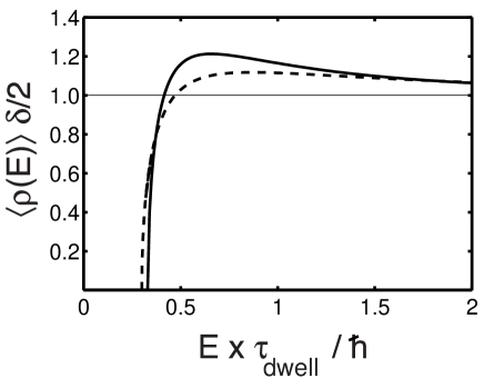
Figure 7: The dashed curve is the $\Gamma=1$ result of Fig. 6, corresponding to a quantum dot with weak impurity scattering (mean free path $l$ much larger than the width $W$ of the point contact). The solid curve is the corresponding result for strong impurity scattering ($l\ll W$). The line shape is almost the same, but the energy scale is different (given by Eqs. (74) and (75), respectively). Adapted from Ref. Vav03 .

The density of states in the two limits is shown in Fig. 7. There is little difference, once the energy is scaled by $\tau_{\rm dwell}$. For $l\gg W$ the excitation gap is given by the RMT result $E_{\rm gap}=0.300\,\hbar/\tau_{\rm dwell}$, cf. Eq. (71). For $l\ll W$ Vavilov and Larkin find $E_{\rm gap}=0.331\,\hbar/\tau_{\rm dwell}$.

VI.4 Magnetic field dependence

A magnetic field $B$, perpendicular to the billiard, breaks time-reversal symmetry, thereby suppressing the excitation gap. A perturbative treatment remains possible as long as $E_{\rm gap}(B)$ remains large compared to $\delta$ Mel97 .

The appropriate RMT ensemble for the isolated billiard is described by the Pandey-Mehta distribution Meh91 ; Pan83

$$P(H) \propto \exp\biggl{(}-\frac{\pi^{2}(1+b^{2})}{4M\delta^{2}}$$ (76)

$$\mbox{}\times\sum_{i,j=1}^{M}\left[({\rm Re}\,H_{ij})^{2}+b^{-2}({\rm Im}\,H_{ij})^{2}\right]\biggr{)}.$$

The parameter $b\in[0,1]$ measures the strength of the time-reversal symmetry breaking. The invariance of $P(H)$ under unitary transformations is broken if $b\neq 0,1$. The relation between $b$ and the magnetic flux $\Phi$ through the billiard is Bee97

$$Mb^{2}=c(\Phi e/h)^{2}\frac{\hbar v_{F}}{\delta\sqrt{A}},$$ (77)

with $c$ a numerical coefficient that depends only on the shape of the billiard. Time-reversal symmetry is effectively broken when $Mb^{2}\simeq g$, which occurs for $\Phi\simeq(h/e)\sqrt{\tau_{\rm erg}/\tau_{\rm dwell}}\ll h/e$. The effect of such weak magnetic fields on the bulk superconductor can be ignored.

Figure 8: Magnetic field dependence of the density of states for the case of a ballistic point contact ($\Gamma_{n}\equiv 1$), computed from Eqs. (65a), (66), and (78). The microscopic gap of order $\delta$ which persists when $\Phi>\Phi_{c}$ is not resolved in this calculation. Adapted from Ref. Mel97 .

The selfconsistency equation for the Green function is the same as Eq. (61), with one difference: On the right-hand-side the terms $G_{12}$ and $G_{21}$ are multiplied by the factor $(1-b^{2})/(1+b^{2})$. In the limit $M\rightarrow\infty$, $b\rightarrow 0$, $Mb^{2}$ finite, the first equation (65a) still holds, but the second equation (65b) is replaced by

$$(2\pi E/\delta-4Mb^{2}G_{11})G_{12}=G_{11}$$

$$\mbox{}\times\sum_{n=1}^{N}(-G_{12}+1-2/\Gamma_{n})^{-1}.$$ (78)

The resulting magnetic field dependence of the average density of states is plotted in Fig. 8, for the case $\Gamma_{n}\equiv 1$ of a ballistic point contact. The gap closes when $Mb^{2}=N\Gamma/8$. The corresponding critical flux $\Phi_{c}$ follows from Eq. (77).

VI.5 Broken time-reversal symmetry

A microscopic suppression of the density of states around $E=0$, on an energy scale of the order of the level spacing, persists even if time-reversal symmetry is fully broken. The suppression is a consequence of the level repulsion between the lowest excitation energy $E_{1}$ and its mirror image $-E_{1}$, which itself follows from the ${\cal CT}$-antisymmetry (55) of the Hamiltonian. Because of this mirror symmetry, the effective Hamiltonian ${\cal H}_{\rm eff}$ of the Andreev billiard can be factorized as

$${\cal H}_{\rm eff}=U\left(\begin{array}[]{cc}{\cal E}&0\\ 0&-{\cal E}\end{array}\right)U^{\dagger},$$ (79)

with $U$ a $2M\times 2M$ unitary matrix and ${\cal E}={\rm diag}(E_{1},E_{2},\ldots E_{M})$ a diagonal matrix containing the positive excitation energies.

Altland and Zirnbauer Alt96 have surmised that an ensemble of Andreev billiards in a strong magnetic field would have a distribution of Hamiltonians of the Wigner-Dyson form (42), constrained by Eq. (79). This constraint changes the Jacobian from the space of matrix elements to the space of eigenvalues, so that the eigenvalue probability distribution is changed from the form (43) (with $\beta=2$) into

$$P(\{E_{n}\})\propto\prod_{i<j}(E_{i}^{2}-E_{j}^{2})^{2}\prod_{k}E_{k}^{2}e^{-V(E_{k})-V(-E_{k})}.$$ (80)

The distribution (80) with $V(E)\propto E^{2}$ is related to the Laguerre unitary ensemble (LUE) of RMT Meh91 by a change of variables. The average density of states vanishes quadratically near zero energy Sle93 ,

$$\langle\rho(E)\rangle=\frac{2}{\delta}\left(1-\frac{\sin(4\pi E/\delta)}{4\pi E/\delta}\right).$$ (81)

All of this is qualitatively different from the “folded GUE” that one would obtain by simply combining two independent GUE’s of electrons and holes Bru95 .

A derivation of Altland and Zirnbauer’s surmise has been given by Frahm et al. Fra96 , who showed that the LUE for the effective Hamiltonian ${\cal H}_{\rm eff}$ of the Andreev billiard follows from the GUE for the Hamiltonian $H$ of the isolated billiard, provided that the coupling to the superconductor is sufficiently strong. To compute the spectral statistics on the scale of the level spacing, a non-perturbative technique is needed. This is provided by the supersymmetric method Efe97 . (See Ref. Gnu03 for an alternative approach using quantum graphs.)

The resulting average density of states is Fra96

$$\langle\rho(E)\rangle = \frac{2}{\delta}-\frac{\sin(2\pi E/\delta)}{\pi E}\int_{0}^{\infty}ds\ e^{-s}$$ (82)

$$\mbox{}\times\cos\left(\frac{2\pi E}{\delta}\sqrt{1+\frac{4s}{g_{A}}}\,\right),$$

$$g_{A} = \sum_{n=1}^{N}\frac{2\Gamma_{n}^{2}}{(2-\Gamma_{n})^{2}}.$$ (83)

The parameter $g_{A}$ is the Andreev conductance of the point contact that couples the billiard to the superconductor Bee92 . The Andreev conductance can be much smaller than the normal-state conductance $g=\sum_{n=1}^{N}\Gamma_{n}$. (Both conductances are in units of $2e^{2}/h$.) In the tunneling limit $\Gamma_{n}\equiv\Gamma\ll 1$ one has $g=N\Gamma$ while $g_{A}=\frac{1}{2}\,N\Gamma^{2}$.

Figure 9: Density of states of the Andreev billiard in a strong magnetic field for three different values of the Andreev conductance of the point contact: $g_{A}=0.4,\ 4,\ 40$. The solid curves are calculated from Eq. (82). The dashed line is the LUE result (81), corresponding to the limit $g_{A}\to\infty$. The dotted line is the GUE limit $g_{A}\rightarrow 0$. Adapted from Ref. Fra96 .

Eq. (9) describes the crossover from the GUE result $\rho(E)=2/\delta$ for $g_{\rm A}\ll 1$ to the LUE result (81) for $g_{\rm A}\gg 1$. The opening of the gap as the coupling to the superconductor is increased is plotted in Fig. 9. The ${\cal CT}$-antisymmetry becomes effective at an energy $E$ for $g_{\rm A}\gtrsim E/\delta$. For small energies $E\ll\delta\,\min(\sqrt{g_{\rm A}},\,1)$ the density of states vanishes quadratically, regardless of how weak the coupling is.

VI.6 Mesoscopic fluctuations of the gap

The smallest excitation energy $E_{1}$ in the Andreev billiard fluctuates from one member of the ensemble to the other. Vavilov et al. Vav01 have surmised that the distribution of these fluctuations is identical upon rescaling to the known distribution Tra94 of the lowest eigenvalue in the Gaussian ensembles of RMT. This surmise was proven using the supersymmetry technique by Ostrovsky, Skvortsov, and Feigelman Ost01 and by Lamacraft and Simons Lam01 . Rescaling amounts to a change of variables from $E_{1}$ to $x=(E_{1}-E_{\rm gap})/\Delta_{\rm gap}$, where $E_{\rm gap}$ and $\Delta_{\rm gap}$ parameterize the square-root dependence (68) of the mean density of states near the gap in perturbation theory. The gap fluctuations are a mesoscopic, rather than a microscopic effect, because the typical magnitude $\Delta_{\rm gap}\simeq E_{\rm gap}^{1/3}\delta^{2/3}$ of the fluctuations is $\gg\delta$ for $E_{\rm gap}\gg\delta$. Still, the fluctuations are small on the scale of the gap itself.

Following Ref. Vav01 , in zero magnetic field the gap distribution is obtained by rescaling the GOE result of Tracy and Widom Tra94 ,

$$P(E_{1})=\frac{d}{dE_{1}}F_{1}\left[(E_{1}-E_{\rm gap})/\Delta_{\rm gap}\right],$$ (84)

$$F_{1}(x)=\exp\left(-{\textstyle\frac{1}{2}}\int_{-\infty}^{x}[q(x^{\prime})+(x-x^{\prime})q^{2}(x^{\prime})]dx^{\prime}\right).$$

(85)

The function $q(x)$ is the solution of

$$q^{\prime\prime}(x)=-xq(x)+2q^{3}(x),$$ (86)

with asymptotic behavior $q(x)\to{\rm Ai}(-x)$ as $x\to-\infty$ [${\rm Ai}(x)$ being the Airy function]. For small $x$ there is a tail of the form

$$P(x)\approx\frac{1}{4\sqrt{\pi}|x|^{1/4}}\exp\left(-{\textstyle\frac{2}{3}}|x|^{3/2}\right),\;\;x\ll-1.$$ (87)

The distribution (84) is shown in Fig. 10 (solid curve). The mean and standard deviation are

$$\langle E_{1}\rangle=E_{\rm gap}+1.21\,\Delta_{\rm gap},\;\;\langle(E_{1}-\langle E_{1}\rangle)^{2}\rangle^{1/2}=1.27\,\Delta_{\rm gap}.$$ (88)

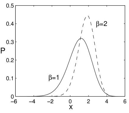
Figure 10: Probability distribution of the rescaled excitation gap $x=(E_{1}-E_{\rm gap})/\Delta_{\rm gap}$, in the presence [$\beta=1$, Eq. (84)] and absence [$\beta=2$, Eq. (89)] of time-reversal symmetry. Adapted from Ref. Vav01 .

Because the mesoscopic fluctuations in the gap occur on a much smaller energy scale $\Delta_{\rm gap}$ than $E_{\rm gap}$, there exists a range of magnetic fields that break time-reversal symmetry of the gap fluctuations without significantly reducing $E_{\rm gap}$ Vav01 . In this field range, specified in Table 1, the distribution of the lowest excitation is given by the GUE result Tra94

$$P(E_{1})=\frac{d}{dE_{1}}F_{2}[(E_{1}-E_{\rm gap})/\Delta_{\rm gap}],$$ (89)

$$F_{2}(x)\exp\left(-\int_{-\infty}^{x}(x-x^{\prime})q^{2}(x^{\prime})dx^{\prime}\right).$$ (90)

This curve is shown dashed in Fig. 10. The tail for small $x$ is now given by

$$P(x)\approx\frac{1}{8\pi|x|}\exp\left(-{\textstyle\frac{4}{3}}|x|^{3/2}\right),\;\;x\ll-1.$$ (91)

Energy scale Flux scale Bulk statistics $\delta$ $(h/e)\tau_{\rm erg}^{1/2}\delta^{1/2}/\hbar^{1/2}$ Edge statistics $E_{\rm gap}^{1/3}\delta^{2/3}$ $(h/e)\tau_{\rm erg}^{1/2}\delta^{1/6}E_{\rm gap}^{1/3}/\hbar^{1/2}$ Gap size $E_{\rm gap}$ $(h/e)\tau_{\rm erg}^{1/2}E_{\rm gap}^{1/2}/\hbar^{1/2}$

Table 1: Characteristic energy and magnetic flux scales for the spectral statistics in the bulk and at the edge of the spectrum and for the size of the gap. The $\beta=2$ distribution (89) applies to the flux range $(h/e)\tau_{\rm erg}^{1/2}\delta^{1/6}E_{\rm gap}^{1/3}/\hbar^{1/2}\ll\Phi\ll(h/e)\tau_{\rm erg}^{1/2}E_{\rm gap}^{1/2}/\hbar^{1/2}$.

The mesoscopic gap fluctuations induce a tail in the ensemble averaged density of states $\langle\rho(E)\rangle$ for $E<E_{\rm gap}$. In the same rescaled variable $x$ the tail is given by Vav01

$$\langle\rho(x)\rangle = -x{\rm Ai}^{2}(x)+[{\rm Ai}^{\prime}(x)]^{2}$$ (92)

$$\mbox{}+{\textstyle\frac{1}{2}}\delta_{\beta,1}{\rm Ai}(x)[1-\int_{x}^{\infty}{\rm Ai}(y)dy].$$

Asymptotically, $\langle\rho(x)\rangle\propto\exp(-\frac{2}{3}\beta|x|^{3/2})$ for $x\ll-1$. The tail in $\langle\rho(E)\rangle$ is the same as the tail in $P(E)$, as it should be, since both tails are due to the lowest eigenvalue. In Fig. 11 we compare these two functions in zero magnetic field, together with the square-root density of states from perturbation theory.

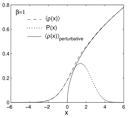
Figure 11: Ensemble averaged density of states $\langle\rho\rangle$ together with the probability distribution $P$ of the excitation gap, as a function of the rescaled energy $x=(E-E_{\rm gap})/\Delta_{\rm gap}$. The dotted and dashed curves are the universal results (84) and (92) of RMT in the presence of time-reversal symmetry ($\beta=1$). The solid curve is the mean density of states (68) in perturbation theory. Adapted from Ref. Vav01 .

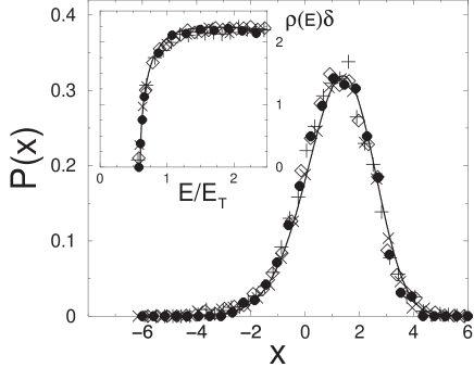
Figure 12: Main plot: Gap distribution for the Andreev kicked rotator with parameters $M=2\pi/\delta=8192$, kicking strength $K=45$, and $M/N=\tau_{\rm dwell}=10$ ($\diamond$), 20 ($\bullet$), 40 ($+$), and 50 ($\times$). There is no magnetic field. The solid line is the RMT prediction (84). Inset: Average density of states for the same system. The solid line is the RMT prediction (71). (Deviations from perturbation theory are not visible on the scale of the inset.) Adapted from Ref. Jac03 .

A numerical simulation of the stroboscopic model of Sec. V provides a test of these predictions Jac03 . Results are shown in Fig. 12, for the case $\beta=1$ and deep in the chaotic regime (kicking strength $K\gg 1$). The agreement with RMT is very good — without any adjustable parameters.

VI.7 Coulomb blockade

Coulomb interactions between electron and hole quasiparticles break the charge-conjugation invariance (55) of the Hamiltonian. Since Andreev reflection changes the charge on the billiard by $2e$, this scattering process becomes energetically unfavorable if the charging energy $E_{C}$ exceeds the superconducting condensation energy (Josephson energy) $E_{J}$. For $E_{C}\gtrsim E_{J}$ one obtains the Coulomb blockade of the proximity effect studied by Ostrovsky, Skvortsov, and Feigelman Ost04 .

The charging energy $E_{C}=e^{2}/2C$ is determined by the capacitance $C$ of the billiard. The Josephson energy is determined by the change in free energy of the billiard resulting from the coupling to the superconductor,

$$E_{J}=-\int_{0}^{\infty}[\rho(E)-2/\delta]\,EdE.$$ (93)

The discrete spectrum $E<E_{\rm gap}$ contributes an amount of order $E_{\rm gap}^{2}/\delta$ to $E_{J}$. In the continuous spectrum $E>E_{\rm gap}$ the density of states $\rho(E)$, calculated by RMT, decays $\propto 1/E^{2}$ to its asymptotic value $2/\delta$. This leads to a logarithmic divergence of the Josephson energy Bro97a ; Asl68 , with a cutoff set by $\min(\Delta,\hbar/\tau_{\rm erg})$:

$$E_{J}=\frac{E_{\rm gap}^{2}}{\delta}\ln\left(\frac{\min(\Delta,\hbar/\tau_{\rm erg})}{E_{\rm gap}}\right).$$ (94)

The suppression of the excitation gap with increasing $E_{C}$ is plotted in Fig. 13, for the case $\Gamma\ll 1$, $\Delta\ll\hbar/\tau_{\rm erg}$ Ost04 . The initial decay is a square root,

$$1-\Delta_{\rm eff}/E_{\rm gap}={\textstyle\frac{1}{2}}\left(\frac{E_{C}\delta}{E_{\rm gap}^{2}\ln(2\Delta/E_{\rm gap})}\right)^{1/2}\ll 1,$$ (95)

and the final decay is exponential,

$$\Delta_{\rm eff}/\Delta=2\exp(-2E_{C}\delta/E_{\rm gap}^{2})\ll 1.$$ (96)

Here $\Delta_{\rm eff}$ refers to the gap in the presence of Coulomb interactions and $E_{\rm gap}=N\Gamma\delta/4\pi$ is the noninteracting value (73).

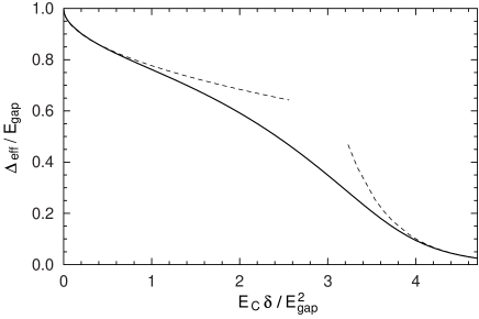
Figure 13: Suppression due to Coulomb interactions of the gap $\Delta_{\rm eff}$ in the density of states of an Andreev billiard coupled by a tunnel junction to a superconductor, relative to the noninteracting gap $E_{\rm gap}=N\Gamma\delta/4\pi$ (with $\Gamma\ll 1\ll N\Gamma$). The plot is for the case $\Delta=e^{5}E_{\rm gap}\ll\hbar/\tau_{\rm erg}$. The dashed lines are the asymptotes (95) and (96). Adapted from Ref. Ost04 .

The gap $\Delta_{\rm eff}$ governs the thermodynamic properties of the Andreev billiard, most importantly the critical current. It is not, however, the relevant energy scale for transport properties. Injection of charge into the billiard via a separate tunnel contact measures the tunneling density of states $\rho_{\rm tunnel}$, which differs in the presence of Coulomb interactions from the thermodynamic density of states $\rho$ considered so far. The gap $\Delta_{\rm tunnel}$ in $\rho_{\rm tunnel}$ crosses over from the proximity gap $E_{\rm gap}$ when $E_{C}\ll E_{J}$ to the Coulomb gap $E_{C}$ when $E_{C}\gg E_{J}$, see Fig. 14. The single peak in $\rho_{\rm tunnel}$ at $\Delta_{\rm tunnel}$ splits into two peaks when $E_{C}$ and $E_{J}$ are of comparable magnitude Ost04 . This peak splitting happens because two states of charge $+e$ and $-e$ having the same charging energy are mixed by Andreev reflection into symmetric and antisymmetric linear combinations with a slightly different energy.

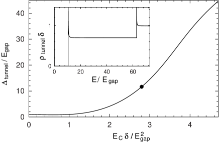
Figure 14: Main plot: gap $\Delta_{\rm tunnel}$ in the tunneling density of states as a function of the charging energy (for $\Delta=e^{5}E_{\rm gap}$ and $N\Gamma=40\,\pi$). The initial decay (barely visible on the scale of the plot) follows Eq. (95) and crosses over to an increase ($\Delta_{\rm tunnel}\rightarrow E_{C}$). Inset: tunneling density of states at $E_{C}\delta/E_{\rm gap}^{2}=2.8$ (corresponding to the dot in the main plot). Adapted from Ref. Ost04 .

VII Quasiclassical theory

It was noticed by Kosztin, Maslov, and Goldbart Kos95 that the classical dynamics at the Fermi energy in an Andreev billiard is integrable — even if the dynamics in the isolated billiard is chaotic. Andreev reflection suppresses chaotic dynamics because it introduces a periodicity into the orbits: The trajectory of an electron is retraced by the Andreev reflected hole. At the Fermi energy the hole is precisely the time reverse of the electron, so that the motion is strictly periodic. For finite excitation energy or in a non-zero magnetic field the electron and the hole follow slightly different trajectories, so the orbit does not quite close and drifts around in phase space Kos95 ; Shy98 ; Wie02 ; Ada02 ; Cse03 .

The near-periodicity of the orbits implies the existence of an adiabatic invariant. Quantization of this invariant leads to the quasiclassical theory of Silvestrov et al. Sil03 .

VII.1 Adiabatic quantization

Figs. 15 and 16 illustrate the nearly periodic motion in a particular Andreev billiard. Fig. 15 shows a trajectory in real space while Fig. 16 is a section of phase space at the interface with the superconductor ($y=0$). The tangential component $p_{x}$ of the electron momentum is plotted as a function of the coordinate $x$ along the interface. Each point in this Poincaré map corresponds to one collision of an electron with the interface. (The collisions of holes are not plotted.) The electron is retroreflected as a hole with the same $p_{x}$. At the Fermi level ($E=0$) the component $p_{y}$ is also the same, and so the hole retraces the path of the electron (the hole velocity being opposite to its momentum). The Poincaré map would then consist of a single point. At non-zero excitation energy $E$ the retroreflection occurs with a slight change in $p_{y}$, because of the difference $2E$ in the kinetic energy of electrons (at energy $E_{F}+E$) and holes (at energy $E_{F}-E$).

Figure 15: Classical trajectory in an Andreev billiard. Particles in a two-dimensional electron gas are deflected by an electrostatic potential. (The dotted circles are equipotentials.) There is specular reflection at the boundaries with an insulator (thick solid lines) and Andreev reflection at the boundary with a superconductor (dashed line). The trajectory follows the motion between two Andreev reflections of an electron near the Fermi energy. The Andreev reflected hole retraces this trajectory in opposite direction. From Ref. Sil03 .

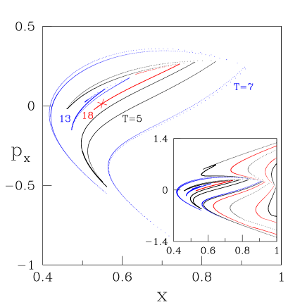
Figure 16: Poincaré map for the Andreev billiard of Fig. 15. Each dot represents a starting point of an electron trajectory, at position $x$ and with tangential momentum $p_{x}$ (in dimensionless units). The inset shows the full surface of section, while the main plot is an enlargement of the central region. The drifting nearly periodic motion follows contours of constant time $T$ between Andreev reflections. The cross marks the starting point of the trajectory shown in the previous figure. From Ref. Sil03 .

The resulting slow drift of the periodic trajectory traces out a contour in the surface of section. These are isochronous contours Sil03 , meaning that the time $T$ between Andreev reflections is the same for each point $x,p_{x}$ on the contour . The adiabatic invariance of $T$ follows from the adiabatic invariance of the action integral $I$ over the nearly periodic motion from electron to hole and back to electron:

$$I=\oint pdq=2ET.$$ (97)

Since $E$ is a constant of the motion, adiabatic invariance of $I$ implies adiabatic invariance of the time $T$ between Andreev reflections.

Adiabatic invariance is defined in the limit $E\rightarrow 0$ and is therefore distinct from invariance in the sense of Kolmogorov-Arnold-Moser (KAM) Gut90 , which would require a critical $E^{*}$ such that a contour is exactly invariant for $E<E^{*}$. There is numerical evidence Kos95 that the KAM theorem does not apply to a chaotic Andreev billiard.

It is evident from Fig. 16 that contours of large $T$ enclose a very small area in a chaotic system. To estimate the area, it is convenient to measure $x$ in units of the width $W$ of the constriction to the superconductor. Similarly, $p_{x}$ is conveniently measured in units of the range $\Delta p$ of transverse momenta inside the constriction. The highly elongated shape evident in Fig. 16 is a consequence of the exponential divergence in time of nearby trajectories, characteristic of chaotic dynamics. The rate of divergence is the Lyapunov exponent $\alpha$. Since the Hamiltonian flow is area preserving, a stretching $\ell_{+}(t)=\ell_{+}(0)e^{\alpha t}$ of the dimension in one direction needs to be compensated by a squeezing $\ell_{-}(t)=\ell_{-}(0)e^{-\alpha t}$ of the dimension in the other direction. The area $A\simeq\ell_{+}\ell_{-}$ is then time independent. Initially, $\ell_{\pm}(0)<1$. The constriction at the superconductor acts as a bottleneck, enforcing $\ell_{\pm}(T)<1$. These two inequalities imply $\ell_{+}(t)<e^{\alpha(t-T)}$, $\ell_{-}<e^{-\alpha t}$. The enclosed area, therefore, has upper bound

$$A_{\rm max}\simeq W\Delta p\,e^{-\alpha T}\simeq\hbar Ne^{-\alpha T},$$ (98)

where $N\simeq W\Delta p/\hbar\gg 1$ is the number of channels in the point contact.

The two invariants $E$ and $T$ define a two-dimensional torus in the four-dimensional phase space. Quantization of this adiabatically invariant torus proceeds following Einstein-Brillouin-Keller Gut90 ; Dun02 , by quantizing the area

$$\oint pdq=2\pi\hbar(m+\nu/4),\;\;m=0,1,2,\ldots$$ (99)

enclosed by each of the two topologically independent contours on the torus. Eq. (99) ensures that the wave functions are single valued. The integer $\nu$ counts the number of caustics (Maslov index) and in this case should also include the number of Andreev reflections.

The first contour follows the quasiperiodic orbit of Eq. (97), leading to

$$ET=(m+{\textstyle\frac{1}{2}})\pi\hbar,\;\;m=0,1,2,\ldots$$ (100)

The quantization condition (100) is sufficient to determine the smoothed (or ensemble averaged) density of states

$$\langle\rho(E)\rangle=N\int_{0}^{\infty}dT\,P(T)\sum_{m=0}^{\infty}\delta\bigl{(}E-(m+{\textstyle\frac{1}{2}})\pi\hbar/T\bigr{)},$$ (101)

using the classical probability distribution $P(T)$ for the time between Andreev reflections. (The distribution $P(T)$ is defined with a uniform measure in the surface of section $(x,p_{x})$ at the interface with the superconductor.)

Eq. (101) is the “Bohr-Sommerfeld rule” of Melsen et al. Mel96 . It generalizes the familiar Bohr-Sommerfeld quantization rule for translationally invariant geometries [cf. Eq. (15)] to arbitrary geometries. The quantization rule refers to classical periodic motion with period $2T$ and phase increment per period of $2ET/\hbar-\pi$, consisting of a part $2ET/\hbar$ because of the energy difference $2E$ between electron and hole, plus a phase shift of $-\pi$ from two Andreev reflections. If $E$ is not $\ll\Delta$, this latter phase shift should be replaced by $-2\arccos(E/\Delta)$ Cse02 ; Cse02b ; Cse04 , cf. Eq. (32). In the presence of a magnetic field an extra phase increment proportional to the enclosed flux should be included Ihr01 . Eq. (101) can also be derived from the Eilenberger equation for the quasiclassical Green function Lod98 .

To find the location of individual energy levels a second quantization condition is needed Sil03 . It is provided by the area $\oint_{T}p_{x}dx$ enclosed by the isochronous contours,

$$\oint_{T}p_{x}dx=2\pi\hbar(n+\nu/4),\;\;n=0,1,2,\ldots$$ (102)

Eq. (102) amounts to a quantization of the period $T$, which together with Eq. (100) leads to a quantization of $E$. For each $T_{n}$ there is a ladder of Andreev levels $E_{nm}=(m+{\textstyle\frac{1}{2}})\pi\hbar/T_{n}$.

While the classical $T$ can become arbitrarily large, the quantized $T_{n}$ has a cutoff. The cutoff follows from the maximal area (98) enclosed by an isochronous contour. Since Eq. (102) requires $A_{\rm max}\gtrsim h$, the longest quantized period is $T_{0}=\alpha^{-1}[\ln N+{\cal O}(1)]$. The lowest Andreev level associated with an adiabatically invariant torus is therefore

$$E_{00}=\frac{\pi\hbar}{2T_{0}}=\frac{\pi\hbar\alpha}{2\ln N}.$$ (103)

The time scale $T_{0}\propto|\ln\hbar|$ is the Ehrenfest time $\tau_{E}$ of the Andreev billiard, to which we will return in Sec. VIII.

The range of validity of adiabatic quantization is determined by the requirement that the drift $\delta x$, $\delta p_{x}$ upon one iteration of the Poincaré map should be small compared to the characteristic values $W,p_{F}$. An estimate is Sil03

$$\frac{\delta x}{W}\simeq\frac{\delta p_{x}}{p_{F}}\simeq\frac{E_{nm}}{\hbar\alpha N}e^{\alpha T_{n}}\simeq(m+{\textstyle\frac{1}{2}})\frac{e^{-\alpha(T_{0}-T_{n})}}{\alpha T_{n}}.$$ (104)

For low-lying levels ($m\sim 1$) the dimensionless drift is $\ll 1$ for $T_{n}<T_{0}$. Even for $T_{n}=T_{0}$ one has $\delta x/W\simeq 1/\ln N\ll 1$.

VII.2 Integrable dynamics

Unlike RMT, the quasiclassical theory is not restricted to systems with a chaotic classical dynamics. Melsen et al. Mel96 ; Mel97 have used the Bohr-Sommerfeld rule (101) to argue that Andreev billiards with an integrable classical dynamics have a smoothly vanishing density of states — without an actual excitation gap. The presence or absence of an excitation gap is therefore a “quantum signature of chaos”. This is a unique property of Andreev billiards. In normal, not-superconducting billiards, it is impossible to distinguish chaotic from integrable dynamics by looking at the density of states. One needs to measure density-density correlation functions for that purpose Haa01 .

Figure 17: Histograms: smoothed density of states of a billiard coupled by a ballistic $N$-mode lead to a superconductor, determined by Eq. (36) and averaged over a range of Fermi energies at fixed $N$. The scattering matrix is computed numerically by matching wave functions in the billiard to transverse modes in the lead. A chaotic Sinai billiard (top inset, solid histogram, $N=20$) is contrasted with an integrable circular billiard (bottom inset, dashed histogram, $N=30$). The solid curve is the prediction (71) from RMT for a chaotic system and the dashed curve is the Bohr-Sommerfeld result (101), with dwell time distribution $P(T)$ calculated from classical trajectories in the circular billiard. Adapted from Ref. Mel97 .

The difference between chaotic and integrable Andreev billiards is illustrated in Fig. 17. As expected, the chaotic Sinai billiard follows closely the prediction from RMT. (The agreement is less precise than for the kicked rotator of Fig. 12, because the number of modes $N=20$ is necessarily much smaller in this simulation.) The density of states of the integrable circular billiard is suppressed on the same mesoscopic energy scale $E_{T}$ as the chaotic billiard, but the suppression is smooth rather than abrupt. Any remaining gap is microscopic, on the scale of the level spacing, and therefore invisible in the smoothed density of states.

That the absence of an excitation gap is generic for integrable billiards can be understood from the Bohr-Sommerfeld rule Mel96 . Generically, an integrable billiard has a power-law distribution of dwell times, $P(T)\propto T^{-p}$ for $T\rightarrow\infty$, with $p\approx 3$ Bau90 ; Bar93 . Eq. (101) then implies a power-law density of states, $\langle\rho(E)\rangle\propto E^{p-2}$ for $E\rightarrow 0$. The value $p=3$ corresponds to a linearly vanishing density of states. An analytical calculation Kor03 of $P(T)$ for a rectangular billiard gives the long-time limit $P(T)\propto T^{-3}\ln T$, corresponding to the low-energy asymptote $\langle\rho(E)\rangle\propto E\ln(E_{T}/E)$. The weak logarithmic correction to the linear density of states is consistent with exact quantum mechanical calculations Mel96 ; Ihr01 .

VII.3 Chaotic dynamics

A chaotic billiard has an exponential dwell time distribution, $P(T)\propto e^{-T/\tau_{\rm dwell}}$, instead of a power law Bau90 . (The mean dwell time is $\tau_{\rm dwell}=2\pi\hbar/N\delta\equiv\hbar/2E_{T}$.) Substitution into the Bohr-Sommerfeld rule (101) gives the density of states Sch99

$$\langle\rho(E)\rangle=\frac{2}{\delta}\,\frac{(\pi E_{T}/E)^{2}\cosh(\pi E_{T}/E)}{\sinh^{2}(\pi E_{T}/E)},$$ (105)

which vanishes $\propto e^{-\pi E_{T}/E}$ as $E\rightarrow 0$. This is a much more rapid decay than for integrable systems, but not quite the hard gap predicted by RMT Mel96 . The two densities of states are compared in Fig. 18.

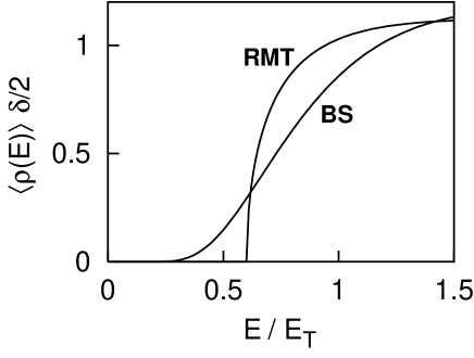
Figure 18: Comparison of the smoothed density of states in a chaotic Andreev billiard as it follows from RMT (Eq. (71), with a hard gap) and as it follows from the Bohr-Sommerfeld (BS) rule (Eq. (105), without a hard gap). These are the two limiting distributions when the Ehrenfest time $\tau_{E}$ is, respectively, much smaller or much larger than the mean dwell time $\tau_{\rm dwell}$.

When the qualitative difference between the random-matrix and Bohr-Sommerfeld theories was discovered Mel96 , it was believed to be a short-coming of the quasiclassical approximation underlying the latter theory. Lodder and Nazarov Lod98 realized that the two theoretical predictions are actually both correct, in different limits. As the ratio $\tau_{E}/\tau_{\rm dwell}$ of Ehrenfest time and dwell time is increased, the density of states crosses over from the RMT form (71) to the Bohr-Sommerfeld form (105). We investigate this crossover in the following section.

VIII Quantum-to-classical crossover

VIII.1 Thouless versus Ehrenfest

According to Ehrenfest’s theorem, the propagation of a quantum mechanical wave packet is described for short times by classical equations of motion. The time scale at which this correspondence between quantum and classical dynamics breaks down in a chaotic system is called the Ehrenfest time $\tau_{E}$ Ber78 . As explained in Fig. 19, it depends logarithmically on Planck’s constant: $\tau_{E}=\alpha^{-1}\ln(S_{\rm cl}/h)$, with $S_{\rm cl}$ the characteristic classical action of the dynamical system and $\alpha$ the Lyapunov exponent.

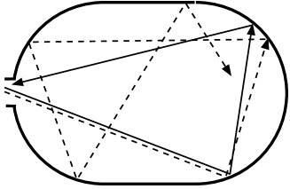
Figure 19: Two trajectories entering a chaotic billiard at a small separation $\delta x(0)$ diverge exponentially in time, $\delta x(t)=\delta x(0)e^{\alpha t}$. The rate of divergence $\alpha$ is the Lyapunov exponent. An initial microscopic separation $\lambda_{F}$ becomes macroscopic at the Ehrenfest time $\tau_{E}=\alpha^{-1}\ln(L^{\ast}/\lambda_{F})$. The macroscopic length $L^{\ast}$ is determined by the size and shape of the billiard. The Ehrenfest time depends logarithmically on Planck’s constant: $\tau_{E}=\alpha^{-1}\ln(S_{\rm cl}/h)$, with $S_{\rm cl}=mv_{F}L^{\ast}$ the characteristic classical action. The evolution of a quantum mechanical wave packet is well described by a classical trajectory only for times less than $\tau_{E}$.

This logarithmic $h$-dependence distinguishes the Ehrenfest time from other characteristic time scales of a chaotic system, which are either $h$-independent (dwell time, ergodic time) or algebraically dependent on $h$ (Heisenberg time $\propto 1/\delta$). That the quasiclassical theory of superconductivity breaks down on time scales greater than $\tau_{E}$ was noticed already in 1968 by Larkin and Ovchinnikov Lar68 .

The choice of $S_{\rm cl}$ depends on the physical quantity which one is studying. For the density of states of the Andreev billiard (area $A$, opening of width $W\ll A^{1/2}$, range of transverse momenta $\Delta p\simeq p_{F}$ inside the constriction) the characteristic classical action is $S_{\rm cl}=mv_{F}W^{2}/A^{1/2}$ Vav03 . The Ehrenfest time then takes the form

$$\tau_{E}=\alpha^{-1}[\ln(N^{2}/M)+{\cal O}(1)].$$ (106)

Here $M=k_{F}A^{1/2}/\pi$ and $N=k_{F}W/\pi$ are, respectively, the number of modes in a cross-section of the billiard and in the point contact. Eq. (106) holds for $N\gtrsim\sqrt{M}$. For $N\lesssim\sqrt{M}$ the Ehrenfest time may be set to zero, because the wave packet then spreads over the entire billiard within the ergodic time Sil03b .

Chaotic dynamics requires $\alpha^{-1}\ll\tau_{\rm dwell}$. The relative magnitude of $\tau_{E}$ and $\tau_{\rm dwell}$ thus depends on whether the ratio $N^{2}/M$ is large or small compared to the exponentially large number $e^{\alpha\tau_{\rm dwell}}$.

The result of RMT Mel96 , cf. Sec. VI.2, is that the excitation gap in an Andreev billiard is of the order of the Thouless energy $E_{T}\simeq\hbar/\tau_{\rm dwell}$. It was realized by Lodder and Nazarov Lod98 that this result requires $\tau_{E}\ll\tau_{\rm dwell}$. More generally, the excitation gap $E_{\rm gap}\simeq{\rm min}\,(E_{T},\hbar/\tau_{E})$ is determined by the smallest of the Thouless and Ehrenfest energy scales. The Bohr-Sommerfeld theory Mel96 , cf. Sec. VII.3, holds in the limit $\tau_{E}\rightarrow\infty$ and therefore produces a gapless density of states.

VIII.2 Effective RMT

A phenomenological description of the crossover from the Thouless to the Ehrenfest regime is provided by the “effective RMT” of Silvestrov et al. Sil03 . As described in Sec. VII.1, the quasiclassical adiabatic quantization allows to quantize only the trajectories with periods $T\leq T_{0}\equiv\tau_{E}$. The excitation gap of the Andreev billiard is determined by the part of phase space with periods longer than $\tau_{E}$. Effective RMT is based on the hypothesis that this part of phase space can be quantized by a scattering matrix $S_{\rm eff}$ in the circular ensemble of RMT, with a reduced dimensionality

$$N_{\rm eff}=N\int_{\tau_{E}}^{\infty}P(T)\,dT=Ne^{-\tau_{E}/\tau_{\rm dwell}}.$$ (107)

Figure 20: Pictorial representation of the effective RMT of an Andreev billiard. The part of phase space with time $T>\tau_{E}$ between Andreev reflections is represented by a chaotic cavity (mean level spacing $\delta_{\rm eff}$), connected to the superconductor by a long lead ($N_{\rm eff}$ propagating modes, one-way delay time $\tau_{E}/2$ for each mode). Between two Andreev reflections an electron or hole spends, on average, a time $\tau_{E}$ in the lead and a time $\tau_{\rm dwell}$ in the cavity. The scattering matrix of lead plus cavity is $\exp(iE\tau_{E}/\hbar)S_{0}(E)$, with $S_{0}(E)$ distributed according to the circular ensemble of RMT (with effective parameters $N_{\rm eff}$, $\delta_{\rm eff}$). The complete excitation spectrum of the Andreev billiard consists of the levels of the effective RMT (periods $>\tau_{E}$) plus the levels obtained by adiabatic quantization (periods $<\tau_{E}$).

The energy dependence of $S_{\rm eff}(E)$ is that of a chaotic cavity with mean level spacing $\delta_{\rm eff}$, coupled to the superconductor by a long lead with $N_{\rm eff}$ propagating modes. (See Fig. 20.) The lead introduces a mode-independent delay time $\tau_{E}$ between Andreev reflections, to ensure that $P(T)$ is cut off for $T<\tau_{E}$. Because $P(T)$ is exponential $\propto\exp(-T/\tau_{\rm dwell})$, the mean time $\langle T\rangle_{\ast}$ between Andreev reflections in the accessible part of phase space is simply $\tau_{E}+\tau_{\rm dwell}$. The effective level spacing in the chaotic cavity by itself (without the lead) is then determined by

$$\frac{2\pi\hbar}{N_{\rm eff}\delta_{\rm eff}}=\langle T\rangle_{\ast}-\tau_{E}=\tau_{\rm dwell}.$$ (108)

It is convenient to separate the energy dependence due to the lead from that due to the cavity, by writing $S_{\rm eff}(E)=\exp(iE\tau_{E}/\hbar)S_{0}(E)$, where $S_{0}(E)$ represents only the cavity and has an energy dependence of the usual RMT form (44) — with effective parameters $N_{\rm eff}$ and $\delta_{\rm eff}$. The determinant equation (36) for the excitation spectrum then takes the form

$${\rm Det}\,\left[1-\alpha(E)^{2}e^{2iE\tau_{E}/\hbar}S_{0}(E)S_{0}(-E)^{\ast}\right]=0.$$ (109)

We can safely replace $\alpha(E)\equiv\exp[-i\arccos(E/\Delta)]\rightarrow-i$ (since $E\ll\Delta$), but the energy dependence of the phase factor $e^{2iE\tau_{E}/\hbar}$ can not be omitted.

Figure 21: Excitation gap of the Andreev billiard in the crossover from Thouless to Ehrenfest regimes. The solid curve is the solution of the effective RMT of Ref. Sil03 , derived in App. A. The dotted lines are the two asymptotes (110) and (111). The dashed curve is the result of the stochastic model of Ref. Vav03 , discussed in Sec. VIII.3.

In App. A we calculate the smallest positive $E$ that solves Eq. (109), which is the excitation gap $E_{\rm gap}$ of the effective RMT. The result is plotted in Fig. 21 (solid curve), as a function of $\tau_{E}/\tau_{\rm dwell}$. The two asymptotes (dotted lines) are

$$E_{\rm gap} = \frac{\gamma^{5/2}\hbar}{\tau_{\rm dwell}}\left(1-(2\gamma-1)\frac{\tau_{E}}{\tau_{\rm dwell}}\right),\;\;\tau_{E}\ll\tau_{\rm dwell},$$ (110)

$$E_{\rm gap} = \frac{\pi\hbar}{2\tau_{E}}\left(1-(3+\sqrt{8})\frac{\tau_{\rm dwell}}{\tau_{E}}\right),\;\;\tau_{E}\gg\tau_{\rm dwell},$$ (111)

with $\gamma=\frac{1}{2}(\sqrt{5}-1)$ the golden number.

The $\tau_{E}$ time delay characteristic of the effective RMT was introduced in Ref. Sil03 , but its effect on the excitation gap was not evaluated properly. As a consequence the formula for the gap given in that paper,

$$E_{\rm gap}=\frac{0.30\,\hbar}{\langle T\rangle_{\ast}}=\frac{0.30\,\hbar}{\tau_{E}+\tau_{\rm dwell}},$$ (112)

provides only a qualitative description of the actual crossover.

Figure 22: The data points (left axis) are the quantum mechanical gap values $E_{\rm gap}$ of the Andreev kicked rotator as a function of the location of the NS interface, for parameter values $M=131072$, $\tau_{\rm dwell}=M/N=5$, $K=14$. The solid curve (right axis) is the reciprocal of the mean dwell time (113) of classical trajectories longer than $T^{*}=7$. Adapted from Ref. Goo03 .

The inverse correlation (112) between the gap and the dwell time of long trajectories was observed in a computer simulation of the Andreev kicked rotator Goo03 . The data points in Fig. 22 track the excitation gap as the location in phase space of the NS interface is varied. The solid curve is a plot of

$$\frac{1}{\langle T\rangle_{\ast}}=\frac{\int_{T^{\ast}}^{\infty}P(T)dT}{\int_{T^{\ast}}^{\infty}TP(T)dT},$$ (113)

with $P(T)$ the classical dwell time distribution and $T^{\ast}=7$. We see that the sample-to-sample fluctuations in the gap correlate very well with the fluctuations in the mean dwell time of long trajectories. The correlation is not sensitive to the choice of $T^{\ast}$, as long as it is greater than $\tau_{E}=4.4$.

VIII.3 Stochastic model

Small-angle scattering by a smooth disorder potential provides a stochastic model for the quantum diffraction of a wave packet in a chaotic billiard Ale96 . The scattering time of the stochastic model plays the role of the Ehrenfest time in the deterministic chaotic dynamics. The advantage of a stochastic description is that one can average over different realizations of the disorder potential. This provides for an established set of analytical techniques. The disadvantage is that one does not know how well stochastic scattering mimics quantum diffraction.

Vavilov and Larkin Vav03 have used the stochastic model to study the crossover from the Thouless regime to the Ehrenfest regime in an Andreev billiard. They discovered that the rapid turn-on of quantum diffraction at $\tau_{E}\gtrsim\tau_{\rm dwell}$ not only causes an excitation gap to open at $\hbar/\tau_{E}$, but that it also causes oscillations with period $\hbar/\tau_{E}$ in the ensemble-averaged density of states $\langle\rho(E)\rangle$ at high energies $E\gtrsim E_{T}$. In normal billiards oscillations with this periodicity appear in the level-level correlation function Ale97 , but not in the level density itself.

The predicted oscillatory high-energy tail of $\langle\rho(E)\rangle$ is plotted in Fig. 23, for the case $\tau_{E}/\tau_{\rm dwell}=3$, together with the smooth results of RMT ($\tau_{E}/\tau_{\rm dwell}\rightarrow 0$) and Bohr-Sommerfeld (BS) theory ($\tau_{E}/\tau_{\rm dwell}\rightarrow\infty$).

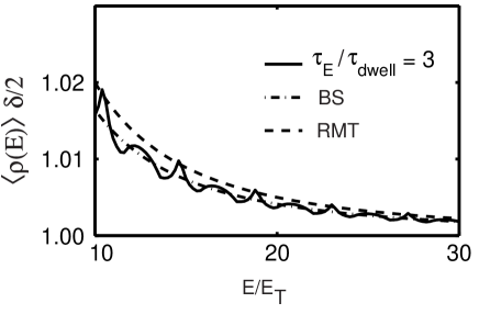
Figure 23: Oscillatory density of states at finite Ehrenfest time (solid curve), compared with the smooth limits of zero (RMT) and infinite (BS) Ehrenfest times. The solid curve is the result of the stochastic model of Vavilov and Larkin, for $\tau_{E}=3\,\tau_{\rm dwell}=3\hbar/2E_{T}$. (The definition (106) of the Ehrenfest time used here differs by a factor of two from that used by those authors.) Adapted from Ref. Vav03 .

Independent analytical support for the existence of oscillations in the density of states with period $\hbar/\tau_{E}$ comes from the singular perturbation theory of Ref. Ada02b . Support from numerical simulations is still lacking. Jacquod et al. Jac03 did find pronounced oscillations for $E\gtrsim E_{T}$ in the level density of the Andreev kicked rotator. However, since these could be described by the Bohr-Sommerfeld theory they can not be the result of quantum diffraction, but must be due to nonergodic trajectories Ihr01b .

The $\tau_{E}$-dependence of the gap obtained by Vavilov and Larkin is plotted in Fig. 21 (dashed curve). It is close to the result of the effective RMT (solid curve). The two theories predict the same limit $E_{\rm gap}\rightarrow\pi\hbar/2\tau_{E}$ for $\tau_{E}/\tau_{\rm dwell}\rightarrow\infty$. The asymptotes given in Ref. Vav03 are

$$E_{\rm gap} = \frac{\gamma^{5/2}\hbar}{\tau_{\rm dwell}}\left(1-0.23\,\frac{\tau_{E}}{2\tau_{\rm dwell}}\right),\;\;\tau_{E}\ll\tau_{\rm dwell},$$ (114)

$$E_{\rm gap} = \frac{\pi\hbar}{2\tau_{E}}\left(1-\frac{2\tau_{\rm dwell}}{\tau_{E}}\right),\;\;\tau_{E}\gg\tau_{\rm dwell}.$$ (115)

Both are different from the results (110) and (111) of the effective RMT.

VIII.4 Numerical simulations

Because the Ehrenfest time grows only logarithmically with the size of the system, it is exceedingly difficult to do numerical simulations deep in the Ehrenfest regime. Two simulations Jac03 ; Kor04 have been able to probe the initial decay of the excitation gap, when $\tau_{E}\lesssim\tau_{\rm dwell}$. We show the results of both simulations in Fig. 24 (closed and open circles), together with the full decay as predicted by the effective RMT of Sec. VIII.2 (solid curve) and by the stochastic model of Sec. VIII.3 (dashed curve).

Figure 24: Ehrenfest-time dependence of the excitation gap in an Andreev billiard, according to the effective RMT (solid curve, calculated in App. A) and according to the stochastic model (dashed curve, calculated in Ref. Vav03 ). The data points result from the simulation of the Andreev kicked rotator Jac03 (closed circles, in the range $N=10^{2}-10^{5}$) and of the Sinai billiard shown in the inset Kor04 (open circles, in the range $N=18-30$).

The closed circles were obtained by Jacquod et al. Jac03 using the stroboscopic model of Sec. V (the Andreev kicked rotator). The number of modes $N$ in the contact to the superconductor was increased from $10^{2}$ to $10^{5}$ at fixed dwell time $\tau_{\rm dwell}=M/N=5$ and kicking strength $K=14$ (corresponding to a Lyapunov exponent $\alpha\approx\ln(K/2)=1.95$). In this way all classical properties of the billiard remain the same while the effective Planck constant $h_{\rm eff}=1/M=1/N\tau_{\rm dwell}$ is reduced by three orders of magnitude. To plot the data as a function of $\tau_{E}/\tau_{\rm dwell}$, Eq. (106) was used for the Ehrenfest time. The unspecified terms of order unity in that equation were treated as a single fit parameter. (This amounts to a horizontal shift by $-0.286$ of the data points in Fig. 24.)

The open circles were obtained by Kormányos et al. Kor04 for the chaotic Sinai billiard shown in the inset. The number of modes $N$ was varied from 18 to 30 by varying the width of the contact to the superconductor. The Lyapunov exponent $\alpha\approx 1.7$ was fixed, but $\tau_{\rm dwell}$ was not kept constant in this simulation. The Ehrenfest time was computed by means of the same formula (106), with $M=2L_{c}k_{F}/\pi$ and $L_{c}$ the average length of a trajectory between two consecutive bounces at the curved boundary segment.

The data points from both simulations have substantial error bars (up to 10%). Because of that and because of their limited range, we can not conclude that the simulations clearly favor one theory over the other.

IX Conclusion

Looking back at what we have learned from the study of Andreev billiards, we would single out the breakdown of random-matrix theory as the most unexpected discovery and the one with the most far-reaching implications for the field of quantum chaos. In an isolated chaotic billiard RMT provides an accurate description of the spectral statistics on energy scales below $\hbar/\tau_{\rm erg}$ (the inverse ergodic time). The weak coupling to a superconductor causes RMT to fail at a much smaller energy scale of $\hbar/\tau_{\rm dwell}$ (the inverse of the mean time between Andreev reflections), once the Ehrenfest time $\tau_{E}$ becomes greater than $\tau_{\rm dwell}$.

In the limit $\tau_{E}\rightarrow\infty$, the quasiclassical Bohr-Sommerfeld theory takes over from RMT. While in isolated billiards such an approach can only be used for integrable dynamics, the Bohr-Sommerfeld theory of Andreev billiards applies regardless of whether the classical motion is integrable or chaotic. This is a demonstration of how the time-reversing property of Andreev reflection unravels chaotic dynamics.

What is lacking is a conclusive theory for finite $\tau_{E}\gtrsim\tau_{\rm dwell}$. The two phenomenological approaches of Secs. VIII.2 and VIII.3 agree on the asymptotic behavior

$$\lim_{\hbar\rightarrow 0}E_{\rm gap}=\frac{\pi\hbar\alpha}{2|\ln\hbar|+{\rm constant}},$$ (116)

in the classical $\hbar\rightarrow 0$ limit (understood as $N\rightarrow\infty$ at fixed $\tau_{\rm dwell}$). There is still some disagreement on how this limit is approached. We would hope that a fully microscopic approach, for example based on the ballistic $\sigma$-model Muz95 ; And96 , could provide a conclusive answer. At present technical difficulties still stand in the way of a solution along those lines Tar01 .

A new direction of research is to investigate the effects of a nonisotropic superconducting order parameter on the Andreev billiard. The case of $d$-wave symmetry is most interesting because of its relevance for high-temperature superconductors. The key ingredients needed for a theoretical description exist, notably RMT Alt02 , quasiclassics Ada02c , and a numerically efficient Andreev map Ada04 .

Appendix A Excitation gap in effective RMT and relationship with delay times

We seek the edge of the excitation spectrum as it follows from the determinant equation (109), which in zero magnetic field and for $E\ll\Delta$ takes the form

$${\rm Det}\,\left[1+e^{2iE\tau_{E}/\hbar}S_{0}(E)S_{0}(-E)^{\dagger}\right]=0.$$ (117)

The unitary symmetric matrix $S_{0}$ has the RMT distribution of a chaotic cavity with effective parameters $N_{\rm eff}$ and $\delta_{\rm eff}$ given by Eqs. (107) and (108). The mean dwell time associated with $S_{0}$ is $\tau_{\rm dwell}$. The calculation for $N_{\rm eff}\gg 1$ follows the method described in Secs. VI.1 and VI.2, modified as in Ref. Bro97a to account for the energy dependent phase factor in the determinant.

Since $S_{0}$ is of the RMT form (44), we can write Eq. (117) in the Hamiltonian form (46). The extra phase factor $\exp(2iE\tau_{E}/\hbar)$ introduces an energy dependence of the coupling matrix,

$${\cal W}_{0}(E)=\frac{\pi}{\cos u}\left(\begin{array}[]{cc}W_{0}W_{0}^{T}\sin u&W_{0}W_{0}^{T}\\ W_{0}W_{0}^{T}&W_{0}W_{0}^{T}\sin u\end{array}\right),$$ (118)

where we have abbreviated $u=E\tau_{E}/\hbar$. The subscript $0$ reminds us that the coupling matrix refers to the reduced set of $N_{\rm eff}$ channels in the effective RMT. Since there is no tunnel barrier in this case, the matrix $W_{0}$ is determined by Eq. (45) with $\Gamma_{n}\equiv 1$. The Hamiltonian

$${\cal H}_{0}=\left(\begin{array}[]{cc}H_{0}&0\\ 0&-H_{0}\end{array}\right)$$ (119)

is that of a chaotic cavity with mean level spacing $\delta_{\rm eff}$. We seek the gap in the density of states

$$\rho(E)=-\frac{1}{\pi}{\rm Im}\,{\rm Tr}\,\left(1+\frac{d{\cal W}_{0}}{dE}\right)(E+i0^{+}-{\cal H}_{0}+{\cal W}_{0})^{-1},$$ (120)

cf. Eq. (53).

The selfconsistency equation for the ensemble-averaged Green function,

$${\cal G}=[E+{\cal W}_{0}-(M\delta_{\rm eff}/\pi)\sigma_{z}G\sigma_{z}]^{-1},$$ (121)

still leads to Eq. (65a), but Eq. (65b) should be replaced by

$$G_{11}+G_{12}\sin u = -(\tau_{\rm dwell}/\tau_{E})uG_{12}$$ (122)

$$\mbox{}\times(G_{12}+\cos u+G_{11}\sin u).$$

(We have used that $N_{\rm eff}\delta_{\rm eff}=2\pi\hbar/\tau_{\rm dwell}$.) Because of the energy dependence of the coupling matrix, the equation (66) for the ensemble averaged density of states should be replaced by

$$\langle\rho(E)\rangle=-\frac{2}{\delta}\,{\rm Im}\,\left(G_{11}-\frac{u}{\cos u}G_{12}\right).$$ (123)

The excitation gap corresponds to a square root singularity in $\langle\rho(E)\rangle$, which can be obtained by solving Eqs. (65a) and (122) jointly with $dE/dG_{11}=0$ for $u\in(0,\pi/2)$. The result is plotted in Fig. 21. The small- and large-$\tau_{E}$ asymptotes are given by Eqs. (110) and (111).

The large-$\tau_{E}$ asymptote is determined by the largest eigenvalue of the time-delay matrix. To see this relationship, note that for $\tau_{E}\gg\tau_{\rm dwell}$ we may replace the determinant equation (117) by

$${\rm Det}\,\left[1+\exp[2iE\tau_{E}/\hbar+2iEQ(0)]+{\cal O}\left(\frac{\tau_{\rm dwell}}{\tau_{E}}\right)^{2}\right]=0.$$ (124)

The Hermitian matrix

$$Q(E)=\frac{1}{i}S_{0}(E)^{\dagger}\frac{d}{dE}S_{0}(E)$$ (125)

is known in RMT as the Wigner-Smith or time-delay matrix. The roots $E_{np}$ of Eq. (124) satisfy

$$2E_{np}(\tau_{E}+\tau_{n})=(2p+1)\pi\hbar,\;\;p=0,1,2,\ldots.$$ (126)

The eigenvalues $\tau_{1},\tau_{2},\ldots\tau_{N_{\rm eff}}$ of $\hbar Q(0)$ are the delay times. They are all positive, distributed according to a generalized Laguerre ensemble Bro98 . In the limit $N_{\rm eff}\rightarrow\infty$ the distribution of the $\tau_{n}$’s is nonzero only in the interval $(\tau_{-},\tau_{+})$, with $\tau_{\pm}=\tau_{\rm dwell}(3\pm\sqrt{8})$. By taking $p=0$, $\tau_{n}=\tau_{+}$ we arrive at the asymptote (111).

The precise one-to-one correspondence (126) between the spectrum of low-lying energy levels of the Andreev billiard and the spectrum of delay times is a special property of the classical limit $\tau_{E}\rightarrow\infty$. For $\tau_{E}\lesssim\tau_{\rm dwell}$ there is only a qualitative similarity of the two spectral densities Cra02 .

References

- (1) A. F. Andreev, Zh. Eksp. Teor. Fiz. 46, 1823 (1964) [Sov. Phys. JETP 19, 1228 (1964)].
- (2) Y. Imry, Introduction to Mesoscopic Physics (Oxford University, Oxford, 2002).
- (3) C. W. J. Beenakker, Rev. Mod. Phys. 69, 731 (1997).
- (4) B. J. van Wees and H. Takayanagi, in Mesoscopic Electron Transport, edited by L. L. Sohn, L. P. Kouwenhoven, and G. Schön, NATO ASI Series E345 (Kluwer, Dordrecht, 1997).
- (5) I. Kosztin, D. L. Maslov, and P. M. Goldbart, Phys. Rev. Lett. 75, 1735 (1995).
- (6) J. Eroms, M. Tolkiehn, D. Weiss, U. Rössler, J. De Boeck, and G. Borghs, Europhys. Lett. 58, 569 (2002).
- (7) M. C. Gutzwiller, Chaos in Classical and Quantum Mechanics (Springer, New York, 1990).
- (8) F. Haake, Quantum Signatures of Chaos (Springer, Berlin, 2001).
- (9) M. L. Mehta, Random Matrices (Academic, New York, 1991).
- (10) T. Guhr, A. Müller-Groeling, and H. A. Weidenmüller, Phys. Rep. 299, 189 (1998).
- (11) P. G. de Gennes, Superconductivity of Metals and Alloys (Benjamin, New York, 1966).
- (12) K. K. Likharev, Rev. Mod. Phys. 51, 101 (1979).
- (13) C. W. J. Beenakker, in: Transport Phenomena in Mesoscopic Systems, edited by H. Fukuyama and T. Ando (Springer, Berlin, 1992); cond-mat/0406127.
- (14) W. L. McMillan, Phys. Rev. 175, 537 (1968).
- (15) P. G. de Gennes and D. Saint-James, Phys. Lett. 4, 151 (1963).
- (16) A. A. Golubov and M. Yu. Kuprianov, J. Low Temp. Phys. 70, 83 (1988).
- (17) W. Belzig, C. Bruder, and G. Schön, Phys. Rev. B 54, 9443 (1996).
- (18) S. Pilgram, W. Belzig, and C. Bruder, Phys. Rev. B 62, 12462 (2000).
- (19) W. Belzig, F. K. Wilhelm, C. Bruder, G. Schön, and A. D. Zaikin, Superlatt. Microstruct. 25, 1251 (1999).
- (20) J. A. Melsen, P. W. Brouwer, K. M. Frahm, and C. W. J. Beenakker, Europhys. Lett. 35, 7 (1996).
- (21) A. Lodder and Yu. V. Nazarov, Phys. Rev. B 58, 5783 (1998).
- (22) C. W. J. Beenakker, Phys. Rev. Lett. 67, 3836 (1991); 68, 1442(E) (1992).
- (23) E. B. Bogomolny, Nonlinearity 5, 805 (1992).
- (24) R. E. Prange, Phys. Rev. Lett. 90, 070401 (2003).
- (25) Ph. Jacquod, H. Schomerus, and C. W. J. Beenakker, Phys. Rev. Lett. 90, 207004 (2003).
- (26) A. Ossipov, T. Kottos, and T. Geisel, Europhys. Lett. 62, 719 (2003).
- (27) Y. V. Fyodorov and H.-J. Sommers, JETP Lett. 72, 422 (2000).
- (28) A. Ossipov and T. Kottos, Phys. Rev. Lett. 92, 017004 (2004).
- (29) F. M. Izrailev, Phys. Rep. 196, 299 (1990).
- (30) J. Tworzydło, A. Tajic, and C. W. J. Beenakker, cond-mat/0405122.
- (31) R. Ketzmerick, K. Kruse, and T. Geisel, Physica D 131, 247 (1999).
- (32) O. Bohigas, M.-J. Giannoni, and C. Schmit, Phys. Rev. Lett. 52, 1 (1984).
- (33) S. Müller, S. Heusler, P. Braun, F. Haake, and A. Altland, nlin.CD/0401021.
- (34) M. G. Vavilov, P. W. Brouwer, V. Ambegaokar, and C. W. J. Beenakker, Phys. Rev. Lett. 86, 874 (2001).
- (35) P. W. Brouwer and C. W. J. Beenakker, Chaos, Solitons & Fractals 8, 1249 (1997). In Eq. (8) of this publication the factor should read and in the right-hand-side of Eq. (15) a factor should be inserted (cf. Eq. (53) in the present paper).
- (36) K. M. Frahm, P. W. Brouwer, J. A. Melsen, and C. W. J. Beenakker, Phys. Rev. Lett. 76, 2981 (1996).
- (37) A. Altland and M. R. Zirnbauer, Phys. Rev. Lett. 76, 3420 (1996); Phys. Rev. B 55, 1142 (1997).
- (38) M. G. Vavilov and A. I. Larkin, Phys. Rev. B 67, 115335 (2003).
- (39) A. Pandey, Ann. Phys. (N.Y.) 134, 110 (1981).
- (40) E. Brézin and A. Zee, Phys. Rev. E 49, 2588 (1994).
- (41) L. A. Pastur, Teoret. Mat. Fiz. 10, 102 (1972) [Theoret. Math. Phys. 10, 67 (1972)].
- (42) M. Tinkham, Introduction to Superconductivity (McGraw-Hill, New York, 1995).
- (43) J. A. Melsen, P. W. Brouwer, K. M. Frahm, and C. W. J. Beenakker, Physica Scripta T69, 223 (1997).
- (44) A. Pandey and M. L. Mehta, Commun. Math. Phys. 87, 449 (1983).
- (45) T. Nagao and K. Slevin, J. Math. Phys. 34, 2075 (1993).
- (46) J. T. Bruun, S. N. Evangelou, and C. J. Lambert, J. Phys. Condens. Matt. 7, 4033 (1995).
- (47) K. Efetov, Supersymmetry in Disorder and Chaos (Cambridge University, Cambridge, 1997).
- (48) S. Gnutzmann, B. Seif, F. von Oppen, and M. R. Zirnbauer, Phys. Rev. E 67, 046225 (2003).
- (49) C. W. J. Beenakker, Phys. Rev. B 46, 12841 (1992).
- (50) C. A. Tracy and H. Widom, Commun. Math. Phys. 159, 151 (1994); 177, 727 (1996).
- (51) P. M. Ostrovsky, M. A. Skvortsov, and M. V. Feigelman, Phys. Rev. Lett. 87, 027002 (2001); JETP Lett. 75, 336 (2002).
- (52) A. Lamacraft and B. D. Simons, Phys. Rev. B 64, 014514 (2001).
- (53) P. M. Ostrovksy, M. A. Skvortsov, and M. V. Feigelman, Phys. Rev. Lett. 92, 176805 (2004).
- (54) L. G. Aslamasov, A. I. Larkin, and Yu. N. Ovchinnikov, Zh. Eksp. Teor. Fiz. 55, 323 (1968) [Sov. Phys. JETP 28, 171 (1969)].
- (55) A. V. Shytov, P. A. Lee, and L. S. Levitov, Phys. Uspekhi 41, 207 (1998).
- (56) J. Wiersig, Phys. Rev. E 65, 036221 (2002).
- (57) I. Adagideli and P. M. Goldbart, Phys. Rev. B 65, 201306 (2002).
- (58) J. Cserti, P. Polinák, G. Palla, U. Zülicke, and C. J. Lambert, Phys. Rev. B 69, 134514 (2004).
- (59) P. G. Silvestrov, M. C. Goorden, and C. W. J. Beenakker, Phys. Rev. Lett. 90, 116801 (2003).
- (60) P. G. Silvestrov, M. C. Goorden, and C. W. J. Beenakker, Phys. Rev. B 67, 241301 (2003).
- (61) K. P. Duncan and B. L. Györffy, Ann. Phys. (N.Y.) 298, 273 (2002).
- (62) J. Cserti, A. Kormányos, Z. Kaufmann, J Koltai, and C. J. Lambert, Phys. Rev. Lett. 89, 057001 (2002).
- (63) J. Cserti, A. Bodor, J. Koltai, and G. Vattay, Phys. Rev. B 66, 064528 (2002).
- (64) J. Cserti, B. Béri, P. Pollner, and Z. Kaufmann, cond-mat/0405404.
- (65) W. Ihra, M. Leadbeater, J. L. Vega, and K. Richter, Europhys. J. B 21, 425 (2001).
- (66) W. Bauer and G. F. Bertsch, Phys. Rev. Lett. 65, 2213 (1990).
- (67) H. U. Baranger, R. A. Jalabert, and A. D. Stone, Chaos 3, 665 (1993).
- (68) A. Kormányos, Z. Kaufmann, J. Cserti, and C. J. Lambert, Phys. Rev. B 67, 172506 (2003).
- (69) H. Schomerus and C. W. J. Beenakker, Phys. Rev. Lett. 82, 2951 (1999).
- (70) G. P. Berman and G. M. Zaslavsky, Physica A 91, 450 (1978).
- (71) B. V. Chirikov, F. M. Izrailev, and D. L. Shepelyansky, Physica D 33, 77 (1988).
- (72) A. I. Larkin and Yu. N. Ovchinnikov, Zh. Eksp. Teor. Fiz. 55, 2262 (1968) [Sov. Phys. JETP 28, 1200 (1969)].
- (73) M. C. Goorden, Ph. Jacquod, and C. W. J. Beenakker, Phys. Rev. B 68, 220501 (2003).
- (74) I. L. Aleiner and A. I. Larkin, Phys. Rev. B 54, 14423 (1996).
- (75) I. L. Aleiner and A. I. Larkin, Phys. Rev. E 55, 1243 (1997).
- (76) I. Adagideli and C. W. J. Beenakker, Phys. Rev. Lett. 89, 237002 (2002).
- (77) W. Ihra and K. Richter, Physica E 9, 362 (2001).
- (78) A. Kormányos, Z. Kaufmann, C. J. Lambert, and J. Cserti, cond-mat/0309306.
- (79) B. A. Muzykantskii and D. E. Khmelnitskii, JETP Lett. 62, 76 (1995).
- (80) A. V. Andreev, B. D. Simons, O. Agam, and B. L. Altshuler, Nucl. Phys. B 482, 536 (1996).
- (81) D. Taras-Semchuk and A. Altland, Phys. Rev. B 64, 014512 (2001).
- (82) A. Altland, B. D. Simons, and M. R. Zirnbauer, Phys. Rep. 359, 283 (2002).
- (83) I. Adagideli, D. E. Sheehy, and P. M. Goldbart, Phys. Rev. B 66, 140512 (2002).
- (84) I. Adagideli and Ph. Jacquod, Phys. Rev. B 69, 020503 (2004).
- (85) P. W. Brouwer, K. M. Frahm, and C. W. J. Beenakker, Phys. Rev. Lett. 78, 4737 (1997); Waves in Random Media, 9, 91 (1999).
- (86) M. G. A. Crawford and P. W. Brouwer, Phys. Rev. E 65, 026221 (2002).