Quantum interference in resonant tunneling and single spin measurements

Abstract

We consider the resonant tunneling through a multi-level system. It is demonstrated that the resonant current displays quantum interference effects due to a possibility of tunneling through different levels. We show that the interference effects are strongly modulated by a relative phase of states carrying the current. This makes it possible to use these effects for measuring the phase difference between resonant states in quantum dots. We extend our model for a description of magnetotransport through the Zeeman doublets. It is shown that, due to spin-flip transitions, the quantum interference effects generate a distinct peak in the shot-noise power spectrum at the frequency of Zeeman splitting. This mechanism explains modulation in the tunneling current at the Larmor frequency observed in scanning tunneling microscope experiments and can be utilized for a single spin measurement.

I Introduction

The resonant tunneling through quantum dots (or impurities) has been investigated both theoretically and experimentally in large amount of works, yet most investigations concentrated on the resonant tunneling through a single quantum level. In the case of the resonant tunneling through many levels one usually considered the total current as a sum of currents through individual levels. In general, however, this procedure cannot be correct due to the quantum interference effects. We illustrate this point with a simple example.

Let us consider the resonant tunneling through a quantum dot coupled with two reservoirs with different chemical potentials, $\mu_{L,R}$. We assume that two levels of the dot, $E_{1,2}$, are inside the potential bias $\mu_{L}-\mu_{R}$ (see Fig. 1). Then the electric current flows from the left (emitter) to the right (collector) reservoirs through the two levels. If we neglect the Coulomb repulsion between the electrons, the total current is given by the Landauer formula

$$I={e\over 2\pi}\int T(E)\,dE\,,$$ (1)

where $T(E)$ is the total transmission. Since any electron from the left reservoir can tunnel to the right reservoirs via these two levels (Fig. 1), the total transmission is given by a sum of two Breight-Wigner amplitudes:

$$T(E)=\left|{\Gamma\over E-E_{1}+i\Gamma}+\eta{\Gamma\over E-E_{2}+i\Gamma}\right|^{2}\,,$$ (2)

where $\Gamma=(\Gamma_{L}+\Gamma_{R})/2$ is a half of the total width. We assume that $\Gamma_{L}=\Gamma_{R}$ (a symmetric dot), and that the tunneling widths are the same for both levels, yet the Breight-Wigner amplitudes can differ in phase. We therefore introduced the factor $\eta$ in (2) which denotes the relative phase of these amplitudes. It can be shown[1] that $\eta$ can take only two values $\pm 1$, the so-called “in” or “out-of-phase” resonances, respectively.

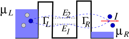
Figure 1: Interference effect in the resonant tunneling through two levels. Here $\Gamma_{L,R}$ denotes the partial width of each of the levels due to tunneling to the left or right reservoir.

It follows from (2) that, if the resonances do not overlap, $\Gamma\ll E_{2}-E_{1}$, the total resonant current is a sum of the resonant currents flowing through the levels $E_{1}$ and $E_{2}$. However, if $\Gamma\sim E_{2}-E_{1}$, the interference plays a very important role in the total resonant current. Indeed, one easily finds that, in the case of constructive interference, $\eta=1$, the total current increases with $\Gamma$ as $I\sim\Gamma$ and, in the case of destructive interference, $\eta=-1$, the total current decreases with $\Gamma$ as $1/\Gamma$. Since in the case of quantum dots the tunneling widths $\Gamma_{L,R}$ can be varied by the corresponding gate voltage, one can use this interference effect in order to measure the relative phase of different levels. This can provide an alternative method for a measurement of this quantity, in addition to that which utilized the Aharonov-Bohm oscillations[2].

The interference effects described above are related to the stationary current. We can also anticipate the interference effects in temporal characteristics of the current. Indeed, it is known that the average resonant current trough a double-dot system would display damped oscillations generated by quantum interference[3]. Since any double-well potential can be mapped to a single well with two levels, one can expect to observe similar damped oscillations in the resonant current flowing through two levels of a single dot. The presence of oscillations in the average current is usually reflected in the current shot-noise power spectrum density, $S(\omega)$. For instance, the resonant current through a double-dot structure would develop a dip in the $S(\omega)$ at the Rabi frequency[4]. Similarly, one can think that the current flowing through two levels (Fig.1) would develop the same structure in $S(\omega)$ at $\omega=E_{2}-E_{1}$. However, the result should strongly depend on the relative phase of two levels. This phase-dependence of the spectral density has not been discussed in the literature, although this effect can have important applications.

The interference effects in resonant tunneling can also be anticipated in the magnetotransport[5]. Indeed, in the presence of magnetic field, all levels in quantum dot or impurity are split (Zeeman splitting). Therefore, electrons in the left reservoir with different orientation of spin (parallel or anti-parallel to the magnetic field) would tunnel to the right reservoir through the different Zeeman sublevels of the dot. This alone cannot result in quantum interference, since the corresponding spin states are orthogonal. However, if the $g$-factor in the dot is different from that in the reservoirs, then the spin-orbit interaction generates the spin-flip of an electron traveling through the quantum dot[5]. As a result, the same electron from the left reservoir flows to the right reservoir through two Zeeman sublevels (Fig.1). Similar to the previous case, one can expect that the related interference effects would be reflected in the behavior of the current spectral density $S(\omega)$. In particular, it was argued in[5] that, in this way, one can explain the puzzled oscillations at Larmour frequency observed in scanning tunneling microscope (STM) experiments[6, 7] and considered as a promising tool for a single spin measurement[8, 9].

In this paper, we investigate the interference effects in resonant tunneling through multilevel systems as quantum dots or impurities. At first sight, the treatment of these effects looks rather straightforward in terms of single electron description [(1) and (2)]. However, this is not the case when the electron-electron repulsion inside the dot is taken into account. In fact, this effect can never be disregarded, and it always plays a very important role in the electron transport. For this reason, one uses the Keldysh nonequilibrium Green’s function technique[10, 11] for an account of the interaction effect in the electron transport. These calculations, however, are rather complicated and are usually performed only in a weak coupling limit. In this paper, we use a different, simpler, and more transparent technique developed by us in Ref. [12]-[15] that consists of reduction of the Schrödinger equation to Bloch-type rate equations for the density matrix obtained by integrating over the reservoir states. Such a procedure can be carried out in the strong nonequilibrium limit without any stochastic assumptions and valid beyond the weak coupling limit. The resulting equations can be used straightforwardly for evaluating the current in a multilevel system and its power spectrum, with the Coulomb repulsion inside the dots taken into account.

The remainder of this paper is as following. In Section II we study the resonant tunneling through two levels of the quantum dot. We obtain the generalized quantum rate equations describing the entire system, including the electric current. Special attention is paid to effect of the relative phase of resonances on the average current and on the shot-noise power spectrum. In Section III, we concentrate on the magnetotransport through quantum dots or impurities. We derive the rate equations for this case and evaluate the shot-noise power spectrum. The obtained results suggest a natural explanation of a peak at the Larmor density and the hyperfine splitting due to interaction with nuclear spin found in new STM measurements. This provides us with a possibility of a single nuclear spin detection. Section IV provides a summary.

II Resonant tunneling through different levels

Let us consider resonant transport in a multilevel system. We shall treat this problem in the framework of a tunnel Hamiltonian approach. Therefore, we introduce the following tunneling Hamiltonian describing the electron transport from the emitter to the collector via different levels of a quantum dot (impurity) $E_{j}$ (Fig. 1), $H=H_{L}+H_{R}+H_{D}+H_{T}$, with

$$H_{L(R)}=\sum_{l(r)}E_{l(r)}a^{\dagger}_{l(r)}a_{l(r)}\,,~{}H_{D}=\sum_{j}E_{j}d^{\dagger}_{j}d_{j}+\hat{U}_{C}\,,$$

$$H_{T}=\Big{(}\sum_{l,j}\Omega^{(j)}_{l}d^{\dagger}_{j}a_{l}+l\leftrightarrow r\Big{)}+H.c.\,.$$ (3)

Here $a^{\dagger}_{l,r}(a_{l,r})$ is the creation (annihilation) operator of an electron in the reservoirs and $d^{\dagger}_{j}(d_{j})$ is the same operator for an electron in the dot (we omitted the spin indices). The operator $\hat{U}_{C}=\sum_{jj^{\prime}}(U_{C}/2)d^{\dagger}_{j}d_{j}d^{\dagger}_{j^{\prime}}d_{j^{\prime}}$ denotes the Coulomb interaction of between electrons in the dot and $\Omega^{(j)}_{l}(\Omega^{(j)}_{r})$ is a coupling between the states $E_{l}(E_{r})$ and $E_{j}$ of the reservoir and the dot, respectively. This coupling is related to the corresponding tunneling width by $\Gamma^{(j)}_{L,R}=2\pi\rho_{L,R}|\Omega^{(j)}_{l,r}|^{2}$, where $\rho_{L,R}$ is the density of states in the corresponding reservoir. (In the absence of magnetic field, one can always choose the gauge such that all couplings $\Omega$ are real).

All parameters of the tunneling Hamiltonian (3) are related to the initial microscopic description of the system in the configuration space ($x$). For instance, the coupling $\Omega^{(j)}_{l(r)}$ is given by the Bardeen formula[16]

$$\Omega^{(j)}_{l(r)}=-{1\over 2m}\int_{{\mbox{\boldmath$x$}}\in\Sigma_{l(r)}}\phi_{j}({\mbox{\boldmath$x$}})\stackrel{{\scriptstyle\leftrightarrow}}{{\nabla}}_{{\mbox{\boldmath$n$}}}\chi_{l(r)}({\mbox{\boldmath$x$}})d\sigma\ ,$$ (4)

where $\phi_{j}({\mbox{\boldmath$x$}})$ and $\chi_{l(r)}({\mbox{\boldmath$x$}})$ are the electron wave functions inside the dot and the reservoir, respectively, and $\Sigma$ is a surface inside the potential barrier that separates the dot from the corresponding reservoir. In one-dimensional (1-D) case $\phi_{j}({\mbox{\boldmath$x$}})\equiv\phi_{j}(x)$ and $\chi_{l(r)}({\mbox{\boldmath$x$}})\equiv\chi_{l(r)}(x)$, (4) can be rewritten as[17]

$$\Omega^{(j)}_{l(r)}=-(\kappa_{j}/m)\phi_{j}(\bar{x}_{l(r)})\chi_{l(r)}(\bar{x}_{l(r)})\,,$$ (5)

where $\kappa_{j}=\sqrt{2m(V(\bar{x})-E_{j})}$. The point $\bar{x}_{l(r)}$ should be taken inside the left (right) barrier and far away from the classical turning points where $\Omega^{(j)}_{l(r)}$ becomes practically independent of $\bar{x}$[18].

It was demonstrated in [12]-[14] that the Schrödinger equation $i\partial_{t}|\Psi(t)\rangle=H|\Psi(t)\rangle$, describing the quantum transport through a multidot system, can be transformed to the Bloch-type rate equation for the reduced density-matrix $\sigma_{\alpha\beta}^{n}(t)\equiv\sigma_{\alpha\beta}^{nn}(t)$, where $|\alpha\rangle,\,|\beta\rangle,\ldots$ are the discrete states of the system in the occupation number representation and $n$ is the number of electrons arriving at the corresponding reservoir by time $t$. This reduction takes place after partial tracing over the reservoir states, and it becomes the exact one in the limit of large bias $\mu_{L}-\mu_{R}\gg\Gamma_{L,R}$ without explicit use of any Markov-type or weak coupling approximations. As a result, the off-diagonal in $n$ density matrix elements, $\sigma_{\alpha\beta}^{nn^{\prime}}(t)$, becomes decoupled from the diagonal in $n$ terms, $\sigma_{\alpha\beta}^{n}(t)$, in the equations of motion[15]. Finally, one arrives at the following Bloch-type equations describing the entire system [14]:

$$\dot{\sigma}_{\alpha\beta}^{n}=i\epsilon_{\beta\alpha}\sigma_{\alpha\beta}^{n}+i\left(\sum_{\gamma}\sigma_{\alpha\gamma}^{n}\tilde{\Omega}_{\gamma\to\beta}-\sum_{\gamma}\tilde{\Omega}_{\alpha\to\gamma}\sigma_{\gamma\beta}^{n}\right)$$

$$-{{\sum}_{\gamma,\delta}}\pi\rho(\sigma_{\alpha\gamma}^{n}\Omega_{\gamma\to\delta}\Omega_{\delta\to\beta}+\sigma_{\gamma\beta}^{n}\Omega_{\gamma\to\delta}\Omega_{\delta\to\alpha})$$

$$+\sum_{\gamma,\delta}\pi\rho\,(\Omega_{\gamma\to\alpha}\Omega_{\delta\to\beta}+\Omega_{\gamma\to\beta}\Omega_{\delta\to\alpha})\sigma_{\gamma\delta}^{n-1}\,,$$ (6)

where $\epsilon_{\beta\alpha}=E_{\beta}-E_{\alpha}$ and $\Omega_{\alpha\to\beta}$ denotes one-electron hopping amplitude that generates $\alpha\to\beta$ transition. We distinguish between the amplitudes $\tilde{\Omega}$ and $\Omega$ of one-electron hopping among isolated states and among isolated and continuum states, respectively. The latter transitions are of the second order in the hopping amplitude $\sim\Omega^{2}$. These transition are produced by two consecutive hoppings of an electron across continuum states with the density of states $\rho$.

Solving (6), we can determine the probability of finding $n$ electrons in the collector, $P_{n}(t)=\sum_{j}\sigma_{jj}^{n}(t)$. This quantity allows us to determine the average current

$$I(t)=e\sum_{n}n\dot{P}(t)\,,$$ (7)

and the current power spectrum. The latter is given by the McDonald formula[19, 5]

$$S(\omega)=2e^{2}\omega\int_{0}^{\infty}dt\sin(\omega t){d\over dt}N_{R}^{2}(t)\,,$$ (8)

where $N_{R}^{2}(t)=\sum_{n}n^{2}P_{n}(t)$.

Consider again the resonant tunneling through the two levels, (Fig.1). Let us assume that the Coulomb repulsion of electrons inside the dot $U_{C}$ is large such that two electrons cannot occupy the dot. Then, there are only three available states of the system, shown in Fig. 2.

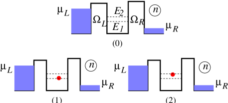
Figure 2: Three available states of the system. Here $n$ denotes the number of electrons arriving at the collector by time $t$.

Let us apply (6) by assigning $\alpha,\beta=\{0,1,2\}$, in an accordance with the states shown in Fig.2. Since the states $1$ and $2$ are not directly coupled, the corresponding hopping amplitude $\tilde{\Omega}=0$ in (6). However, these states can be connected through the reservoirs [the third and the forth terms of (6)]. We assume that the corresponding couplings are weakly dependent on the energy, so that $|\Omega_{l,r}^{(1)}|=|\Omega_{l,r}^{(2)}|=|\Omega_{L,R}|$. However, the sign of the $\Omega_{L,R}^{(1)}$ may be the opposite one with respect to the sign of $\Omega_{L,R}^{(2)}$. Note that, in the 1-D case, a sign of the product $\Omega^{(j)}_{L}\Omega^{(j)}_{R}$ is determined by a sign of the product $\phi_{j}(\bar{x}_{l})\phi_{j}(\bar{x}_{r})$, [see (5)]. The latter can be positive or negative, depending on the number of nodes of $\phi_{j}(x)$ inside the dot[1]. Thus, for a 1-D dot, the product $\Omega^{(j)}_{L}\Omega^{(j)}_{R}$ changes its sign when $j\to j+1$. The reason is that the corresponding wave functions $\phi_{j}(x)$ and $\phi_{j+1}(x)$ differ by an additional node. Hence, the ratio

$$\eta={\Omega^{(j+1)}_{L}\Omega^{(j+1)}_{R}\over\Omega^{(j)}_{L}\Omega^{(j)}_{R}}$$ (9)

is $-1$ for a 1-D dot. However, in the case of a three-dimensional (3-D) quantum dot, where the corresponding coupling $\Omega$ is given by (4), this condition does not hold.

Taking into account (9) one obtains from (6) the following quantum rate equations describing the electron transport through two levels

$$\dot{\sigma}_{00}^{n} = -2\Gamma_{L}\sigma_{00}^{n}+\Gamma_{R}(\sigma_{11}^{n-1}+\sigma_{22}^{n-1})$$ (10a)

$$~{}~{}~{}~{}~{}~{}~{}~{}~{}~{}~{}~{}~{}~{}~{}~{}~{}~{}~{}~{}~{}~{}~{}~{}~{}+\eta\Gamma_{R}(\sigma_{12}^{n-1}+\sigma_{21}^{n-1})$$

$$\dot{\sigma}_{11}^{n} = -\Gamma_{R}\sigma_{11}^{n}+\Gamma_{L}\sigma_{00}^{n}-\eta{\Gamma_{R}\over 2}(\sigma_{12}^{n}+\sigma_{21}^{n})$$ (11a)

$$\dot{\sigma}_{22}^{n} = -\Gamma_{R}\sigma_{22}^{n}+\Gamma_{L}\sigma_{00}^{n}-\eta{\Gamma_{R}\over 2}(\sigma_{12}^{n}+\sigma_{21}^{n})$$ (12a)

$$\dot{\sigma}_{12}^{n} = i\epsilon\sigma_{12}^{n}-\Gamma_{R}\sigma_{12}^{n}+\Gamma_{L}\sigma_{00}^{n}-\eta{\Gamma_{R}\over 2}(\sigma_{11}^{n}+\sigma_{22}^{n}),$$ (13a)

where $\sigma^{n}_{21}=(\sigma^{n}_{12})^{*}$ and $\epsilon=E_{2}-E_{1}$. In these equations, we assumed that $\Omega^{(1)}_{L}=\Omega^{(2)}_{L}$, so that $\eta=\Omega^{(1)}_{R}/\Omega^{(2)}_{R}$. In the case of a different gauge, $\Omega^{(1)}_{R}=\Omega^{(2)}_{R}$ and $\eta=\Omega^{(1)}_{L}/\Omega^{(2)}_{L}$, the factor $\eta$ would appear only in front of the width $\Gamma_{L}$ in (13a). This of course does not affect the final result.

Equations (10a)-(13a can be interpreted in terms of “loss” and “gain” terms, and, therefore, they represent the quantum rate equations. For instance, the first (loss) term in (10a) describes decay of state (0) in Fig.2 due to tunneling of one electron from the left reservoir to the dot. The second (gain) term of the same equation describes decay of states (1) and (2) to state (0). The last (gain) term describes decay of the linear superposition of states (1) and (2). It is given by the product of the corresponding hopping amplitudes from the levels $E_{1,2}$ to the collector reservoir. Since these amplitudes can differ by a sign, this term is proportional the relative phase $\eta$ between the states $E_{1}$ and $E_{2}$.

It is important to note that all transitions in (10a) take place through available continuum states. Therefore, the terms $\sigma_{11}^{n}$ and $\sigma_{22}^{n}$ in (11a) and (12a) can couple with the off-diagonal matrix elements $\sigma_{12}^{n}$ through the right reservoir only. The coupling via the left reservoir would be possible for noninteracting electrons through a new state ($3$) corresponding to two electrons occupying the levels $E_{1}$ and $E_{2}$. The rate equations in this case would be totally symmetric with respect to an interchange of $\Gamma_{L}$ and $\Gamma_{R}$, and the result will coincide with that of the single electron description, [see (1) and (2)]. Note also that, in the case of $\eta=-1$, the two-level system, shown in Figs. 1,2, can be mapped to a coupled-dot system. Then (10a) turn into the system of quantum rate equations, found earlier for a description of electron transport through the coupled-dot system[12, 20].

On can find that the factor $\eta=\pm 1$, in (10a) has the same meaning as the relative phase $\eta$ of two Breit-Wigner amplitudes in Eq. (2). Indeed, it is always $-1$ for two subsequent resonances in one dimensional case. However, in a 3-D quantum dot, the two subsequent resonances can be found in the same phase, depending on particular properties of the quantum dot. One even predicts a whole sequence of the resonances with the same phases[1, 21]. Thus, a measurement of the resonance phase $\eta$ could supply us with additional information on a quantum dot (impurity) structure, complementary to spectroscopic measurements.

Consider first the total current, $I(t)=aI_{L}(t)+bI_{R}(t)$, where $I_{L,R}(t)$, [see (7)] are the currents in the left or in the right reservoirs. The coefficients $a$ and $b$ with $a+b=1$ depend on each junction capacitance[22]. For simplicity we consider only a case where the current in the right reservoir dominates, $b\gg a$. One easily obtains from (10a) that

$$I(t)=e\Gamma_{R}[\sigma_{11}(t)+\sigma_{22}(t)+2\eta\,{\mbox{Re}}\,\sigma_{12}(t)]\,,$$ (14)

where $\sigma_{\alpha\beta}(t)=\sum_{n}\sigma_{\alpha\beta}^{n}(t)$.

Performing summation over $n$ in (10a) and solving these equations in the stationary limit, $t\to\infty$, one easily finds for the stationary current $I=I(t\to\infty)$

$$I/e={2\epsilon^{2}\Gamma_{L}\Gamma_{R}\over\epsilon^{2}\Gamma_{R}+2\Gamma_{L}[\epsilon^{2}+(1-\eta)\Gamma_{R}^{2}]}\,.$$ (15)

(Note that the stationary current is independent on the capacitance of junctions, $a$ and $b$).

As expected, when the resonances begin overlap, the current becomes very sensitive on a sign of the relative phase $\eta$. This is illustrated Fig. 3(a), where we plot the stationary current $I$ as a function of the widths $\Gamma_{R}$. One finds that the current $I$ decreases with $\Gamma_{R}$ if $\eta=-1$ and increases with $\Gamma_{R}$ if $\eta=1$.

Figure 3: Total current through two resonance levels (a) as a function of the width $\Gamma_{R}$ for $\Gamma_{L}=0.5\epsilon$ and (b) as a function of the width $\Gamma_{L}$ for $\Gamma_{R}=0.5\epsilon$.

However, the dependence of the total current $I$ on the width $\Gamma_{L}$ [Fig.3(b)] is rather unexpectable. One finds that the current increases for both values of $\eta$. This is very different from the case of non-interaction electrons [(1) and (2)] where the current is symmetric under an interchange of $\Gamma_{L}$ and $\Gamma_{R}$. Such an asymmetry in the case of interacting electrons is a result of the Coulomb blockade effect[12, 20]. Indeed, an electron enters the dot from the left reservoir with the rate $2\Gamma_{L}$. However, it leaves it with the rate $\Gamma_{R}$, since the state where the two levels $E_{1,2}$ are occupied is forbidden due to electron-electron repulsion. These results can be verified experimentally in the case of a quantum dot, where the width $\Gamma_{L,R}$ can be varied by changing the corresponding gate voltage. Then the relative phase $\eta$ can be obtained from observing the behavior of the resonant current with $\Gamma_{R}$ [Fig. 3(a)].

The quantum interference effects appear as well in the time-dependent current. Let us calculate $I(t)$ [(14)] by solving [(10a)] with the initial conditions $\sigma_{jj^{\prime}}(0)=\delta_{j0}\delta_{j^{\prime}0}$ corresponding to the empty dot. The time-dependent average current is shown in Fig. 4 for $\Gamma_{L}=\epsilon$ and $\Gamma_{R}=0.1\epsilon$ for two values of the relative phase, $\eta=\pm 1$. One finds from this figure that the current displays strong oscillations in contrast with resonant

Figure 4: Time dependence of the resonant current flowing through two resonant levels $E_{1}$ and $E_{2}$, for $\Gamma_{L}=\epsilon$ and $\Gamma_{R}=0.1\epsilon$. The solid line corresponds to the resonances in phase, $\eta=1$, and the dashed line to the off-phase resonances, $\eta=-1$. The dot is empty for $t=0$.

tunneling through a single level. The influence of the relative phase $\eta$ on the quantum oscillations is very substantial. Indeed, the oscillations related to different values of $\eta$ are shifted by half of the period and, moreover, the corresponding dampings are quite different.

The oscillations in the average current are reflected in the shot-noise power spectrum given by $S(\omega)=aS_{L}(\omega)+bS_{R}(\omega)-abS_{Q}(\omega)$[5]. Here $S_{L,R}$ is the current power spectrum in the left (right) reservoir, [(8)] and $S_{Q}(\omega)$ is the charge correlation function of the quantum dot. The latter can also be obtained from (10a). Again, we take for simplicity the case of $b\gg a$, so that $S(\omega)=S_{R}(\omega)$. Then one easily finds from (8) and (10a) that

$$S(\omega)=2e^{2}\omega\Gamma_{R}{\mbox{Im}}\,[Z_{11}(\omega)+Z_{22}(\omega)+Z_{12}(\omega)+Z_{21}(\omega)]\,,$$ (16)

where

$$Z_{\alpha\beta}(\omega)=\int_{0}^{\infty}\sum_{n}(2n+1)\sigma_{\alpha\beta}^{n}(t)\exp(i\omega t)dt\,.$$ (17)

These quantities are obtained directly from (10a) by reducing them to the system of linear algebraic equations.

Using (16), we calculate the ratio of the shot-noise power spectrum to the Schottky noise $S(\omega)/2eI$ (Fano factor), where $I$ is given by (15). This quantity is shown in Fig. 5 for $\Gamma_{L}=\epsilon$ and $\Gamma_{R}=0.1\epsilon$, which are the same parameters as in Fig. 4, and $\eta=\pm 1$. As expected, the quantum interference is reflected in the shot-noise power spectrum. We find that the corresponding Fano factor shows a peak at $\omega=\epsilon$ in the case of “in-phase” resonances and a dip for out-of-phase resonances. Although Fig. 5 displays the Fano factor for an asymmetric quantum dot, $\Gamma_{L}>\Gamma_{R}$, such a strong influence of the phase on the shot-noise power spectrum pertains in a general case. The effect is merely more pronounced for the asymmetric dot. The reason is the Coulomb repulsion that prevents two electron from occupying the dot (c.f. with Fig. 3). For noninteracting electrons ($U_{C}=0$), however, the effect is mostly pronounced for a symmetric case, $\Gamma_{L}=\Gamma_{R}$.

Figure 5: Fano factor versus $\omega$ for the resonant current through two levels. The parameters are the same as in Fig. 4.

Obviously, the shot-noise spectrum of resonant current through a double-dot system should be similar to that shown in Fig. 5 for $\eta=-1$. Indeed, such a system is mapped to a single dot with two levels, corresponding to the symmetric (nodeless) and antisymmetric (one-node) states. Therefore the corresponding shot-noise power spectrum would always show a dip at Rabi frequency (cf.[4]), in contrast with earlier evaluations, which predicted a peak[23].

Our results suggest that the measurement of shot-noise spectrum can be used for a measurement of the relative phase $\eta$. Technically, it would be more complicated than the measurement of the total current as a function of $\Gamma_{R}$ (Fig. 3), which also determines $\eta$, yet the measurement of $S(\omega)$ does not distort the dot, and the phase $\eta$ can be determined even for non-overlapping resonances, $\Gamma_{L,R}\ll\epsilon$.

III Interference effects in magneto-transport

Consider now the electron transport through a quantum dot or impurity in the presence of magnetic field. In this case, all of the levels of the quantum dot are doubled due to the Zeeman splitting (Fig. 6). Then an electron with spin-up can tunnel only through the upper level (Fig. 6). Respectively, an electron with spin-down tunnels only through the lower level. No interference takes place in this case. However, if $g$-factors in the quantum dot and in the reservoirs are different, the tunneling transitions are accompanied by the spin flip[5]. Then the same electron can tunnel from the left to the right reservoir via two level (cf. with Fig. 1). This process would generate oscillations in the resonant current in the same way as was discussed in the previous section.

Let us evaluate the corresponding tunneling amplitudes, which we denote as $\Omega_{L,R}$ and $\delta\Omega_{L,R}$, respectively, for no spin-flip and spin-flip transitions (Fig. 6). This can be done by using (4). Consider for the definiteness the electron transitions between the dot and the right reservoir. The corresponding reservoir wave function $\chi_{R}({\mbox{\boldmath$r$}})$ of (4) is represented by a Kramers doublet $\chi_{R}({\mbox{\boldmath$x$}})=u_{R}({\mbox{\boldmath$r$}})|\uparrow\rangle+v_{R}({\mbox{\boldmath$r$}})|\downarrow\rangle$, where $u_{R}$ and $v_{R}$ are functions of spatial coordinate $r$ only. Therefore, the tunneling matrix elements corresponding to the transitions from the resonant level to the right reservoir without spin flip and accompanied by spin flip are[5]

$$\left(\IEEEeqnarraybox*[][c]{,c,}\Omega_{R}\\ \delta\Omega_{R}\right)=-1/(2m)\int_{{\mbox{\boldmath$r$}}\in\Sigma_{R}}\phi({\mbox{\boldmath$r$}})\stackrel{{\scriptstyle\leftrightarrow}}{{\nabla}}_{{\mbox{\boldmath$n$}}}\left(\IEEEeqnarraybox*[][c]{,c,}u_{R}({\mbox{\boldmath$r$}})\\ v_{R}({\mbox{\boldmath$r$}})\right)d{{\mbox{\boldmath$\sigma$}}}$$ (18)

For relatively small deviations of $g$ factor in the right reservoir from $2$, $|v|\sim O(|\Delta gu|)$, $\Delta g=g-2$,[24], and so the two transition amplitudes are related as $|\delta\Omega_{R}|\sim O(|\Delta g\Omega_{R}|)$. For $\Delta g>1$, the two components $u_{r}$ and $v_{r}$ are of the same order of magnitude and so $\delta\Omega_{R}\sim\Omega_{R}$. The corresponding tunneling amplitudes from the resonant level and the left reservoir are evaluated in the same way.

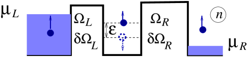
Figure 6: Electron current through an impurity in the presence of magnetic field. Here $\epsilon$ denotes Zeeman splitting and $n$ is the number of electrons that have arrived at the right reservoir (collector) by time $t$.

Now we can obtain the quantum rate equations for magnetotransport through the Zeeman doublet (Fig. 6). We denote $\delta\Omega_{L,R}=\alpha_{L,R}\Omega_{L,R}$, where the coefficients $\alpha_{L,R}$ are of the order of $\Delta g/g$. One finds that, although sign[$\delta\Omega_{L,R}$]=$\pm 1$, the product $\delta\Omega_{L}\delta\Omega_{R}>0$. Thus, the resonances belonging to the Zeeman doublet are always in phase ($\eta=1$). It is convenient to write rate equations separately for electrons polarized up and down in the emitter and collector. Let us consider the polarized up current in the emitter and the collector (Fig. 6). Using (6), we obtain the following rate equations for the reduced density matrix $\sigma_{\alpha\beta}^{n}(t)$ described the spin-polarized transport throgh the Zeeman doublet (the index $n$ denotes the number of electrons with spin up that have arrived at the right reservoir by time $t$):

$$\dot{\sigma}_{00}^{n} = -\Gamma_{L}(1+\alpha_{L}^{2})\sigma_{00}^{n}$$ (19a)

$$+ \Gamma_{R}(\sigma_{11}^{n-1}+\sigma_{22}^{n})+\alpha_{R}^{2}\Gamma_{R}(\sigma_{11}^{n}+\sigma_{22}^{n-1})$$

$$- \alpha_{R}\Gamma_{R}(\sigma_{12}^{n-1}+\sigma_{21}^{n-1}-\sigma_{12}^{n}-\sigma_{21}^{n})$$

$$\ \dot{\sigma}^{n}_{11} = -\Gamma_{R}(1+\alpha_{R}^{2})\sigma^{n}_{11}+\Gamma_{L}\sigma^{n}_{00}$$ (20a)

$$\dot{\sigma}^{n}_{22} = -\Gamma_{R}(1+\alpha_{R}^{2})\sigma^{n}_{22}+\alpha_{L}^{2}\Gamma_{L}\sigma^{n}_{00}$$ (21a)

$$\dot{\sigma}^{n}_{12} = i\epsilon\sigma^{n}_{12}-\Gamma_{R}(1+\alpha_{R}^{2})\sigma^{n}_{12}-\alpha_{L}\Gamma_{L}\sigma^{n}_{00}$$ (22a)

Here we took into account that the spin-flip transitions amplitudes, $\delta\Omega$, from the upper and lower levels of the quantum dot (Fig. 6) are of the opposite sign. Similar to (10a) of the previous section, the quantum interference is generated by transitions between the states of the Zeeman doublet via the reservoirs.

Using (7) and (19a), one obtains for the spin-up polarized current in the right reservoir

$$I(t)=\Gamma_{R}[\sigma_{11}(t)+\sigma_{22}(t)-\alpha_{R}\sigma_{12}(t)-\alpha_{R}\sigma_{21}(t)]\,,$$ (23)

where $\sigma_{\alpha\beta}(t)=\sum_{n}\sigma_{\alpha\beta}^{n}(t)$. The corresponding shot-noise power spectrum $S(\omega)$ is given by the McDonald formula (8). Using (19a), we obtain

$$S(\omega) = 2e^{2}\omega\Gamma_{R}{\mbox{Im}}\,\left\{Z_{11}(\omega)+\alpha_{R}^{2}Z_{22}(\omega)\right.$$ (24)

$$\left.~{}~{}~{}~{}~{}~{}~{}~{}~{}~{}~{}~{}~{}~{}~{}~{}~{}~{}~{}~{}-\alpha_{R}[Z_{12}(\omega)+Z_{21}(\omega)]\right\},$$

where $Z_{\alpha\beta}(\omega)$ is given by (17). The corresonding Fano factor $S(\omega)/2eI$, where $I=I(t\to\infty)$, is therefore determined by (23) and (24).

We display in Fig. 7 the Fano factor as a function of $\omega$ for an asymmetric quantum dot, with the parameters $\Gamma_{L}=\epsilon$, $\Gamma_{R}=0.1\epsilon$ and $\alpha_{L}=\alpha_{R}=0.2$. This quantity shows a clear peak at frequency close to the Zeeman splitting[5]. Similar to the previous case, discussed in Section II, the effect is mostly pronounced for an asymmetric dot due to the influence of Coulomb repulsion. Also, we would like to emphasize that the two resonances of the Zeeman doublet are “in phase”, so that $\eta=1$. Therefore, the shot-noise power spectrum cannot be compared with that of the current through a couple-dot structure. The latter corresponds to $\eta=-1$ and, therefore, the corresponding current spectrum would always display a dip[4], as shown in Fig. 5.

Figure 7: Fano factor versus $\omega$ for the spin-polarized magnetotransport current through the Zeeman doublet, shown in Fig. 6.

We argued in[5] that the interference effect in the resonant tunneling through impurities, considered in the present study, can explain coherent oscillations with Larmor frequency in the STM current. These oscillations were observed in a set of STM experiments as a peak in the tunneling current power spectrum[6, 7], probably in the spin-polarized component of the current[9]. In fact, there have been several attempts to explain the experiments[6], [25]-[28]. All these explanations were based on an assumption that the oscillations of the tunneling current are generated by precession of a localized spin 1/2, interacting with tunneling electrons. In contrast with these models, we suggest that it is not the impurity spin but the current itself that develops coherent oscillations due to tunneling of electrons with via the resonant levels of impurity, spilt by the magnetic field. Indeed, these oscillation would look like those generated by a single spin precession, since the Zeeman splitting coincides with the Larmor frequency. However, there is no precessing spin in our explanation, but only the interference effect of electrons moving through two different states[5].

An essential requirement for our explanation should be a sizable spin-orbit coupling effect. This would imply that the $g$-factor near impurity is different from those inside the bulk and in the tip. This might be due to low space symmetry of an impurity on the surface[29]. Also, the nature of the tip can play a major role, so that the $g$-factor of the tip would depend strongly on the tip radius[30].

It follows from our arguments that the peak in the STM current spectrum is not an evidence of a single spin detection, but rather an effect of coherent resonant scattering (tunneling) on impurity. Nevertheless, the above described spin-coherence mechanism can be used for a single nuclear spin detection, as was suggested in[5]. Indeed, due to the hyperfine coupling, each electronic level will be split into a number of sub-levels. Then, according to our model, the peak in STM current spectrum would be split in a number of peaks corresponding to transitions between various hyperfine levels. Such a splitting, in fact, has already been observed in recent measurements[9]. The data clearly displays different peaks in the current power spectrum – evidence of hyperfine splitting. These experimental results strongly supports our explanation and opens a new way for a measurement of single nuclear spin[5, 9, 30].

IV Conclusion

In this paper, we studied the interference effects in quantum transport through quantum dots or impurities, where the transport is carried via several levels. In our investigation, we used a new method of quantum rate equations which is mostly suitable for treatment of this type of problems and accounts the Coulomb repulsion in a simple and precise way. We found that the interference effects strongly affect the total current as well as the current power spectrum and depend on the relative phase of the levels, carrying the current. For instance, in the case of out-of-phase resonances, the total current drops down when the coupling with the collector increases. This contraintuitive result represents an effect of the destructive interference. On the other hand, no destructive interference effect would appear when one increases the coupling with the emitter. Such an unexpected asymmetry between the emitter and the collector does not appear in the case of non-interacting electrons.

We have also demonstrated that the interference effects are reflected in the shot-noise power spectrum of the resonant current. We found that this quantity depends very strongly on the relative phase of the resonances. It shows a peak for in-phase resonances and a dip for out-of-phase resonances. This opens a possibility for studying the internal structure of quantum dots or impurities by measuring the shot-noise spectrum of the current flowing through these systems.

Finally, we applied our method for study the interference effect in magnetotransport. We showed that, due to the spin-orbit interaction, the electric current would display the interference effects of the same nature as in the tunneling through two levels, separated by the Zeeman spitting. We suggest that this phenomenon can explain the modulation of STM current found in different experiments and attributed to the Larmor precession of the localized spin. Yet, according to our model, these experiments display the interference effect. The hyperfine splitting of the signal into several peaks, found in recent experiments, confirms our model and gives a possibility to use the interference effect as a new effective tool for a single spin measurements.

V Acknowledgment

The authors is grateful to G. Berman, L. Fedichkin, M. Heiblum, and D. Mozyrsky for helpful discussions. The author also acknowledges very useful correspondence with C. Durcan.

Shmuel A. Gurvitz received the Ph.D. from the Institute of Theoretical and Experimental Physics (ITEP), Moscow, Russia, in 1970. Since 1972, he has been with the Weizmann Institute of Science, Rehovot, Israel, where he is currently a Professor of Physics with the Department of Particle Physics. His research interests include Quantum measurements and decoherence, mesoscopic transport, multidimensional and cluster tunneling, and deep inelastic scattering.

References

- [1] G. Hackenbroich, “Phase coherent transmission through interacting mesoscopic systems”, Phys. Rep., vol. 343, pp. 463-538, 2001.
- [2] A. Yacoby, M. Heiblum, D. Mahalu, and Hadas Shtrikman, “Coherence and Phase Sensitive Measurements in a Quantum Dot”, Phys. Rev. Lett., vol. 74, pp. 4047-4050, 1995.
- [3] S.A. Gurvitz, “Josephson-type effect in resonant-tunneling heterostructures” Phys. Rev., vol. B44, pp. 11924-11932, 1991.
- [4] N.B. Sun and G.L. Milburn, “Quantum open-systems approach to current noise in resonant tunneling junctions”, Phys. Rev., vol. B59, pp. 10748-10756, (1999); R. Aguado and T. Brandes, “Shot Noise Spectrum of Open Dissipative Quantum Two-level Systems”, Phys. Rev. Lett., in press.
- [5] D. Mozyrsky, L. Fedichkin, S. A. Gurvitz, and G. P. Berman, “Interference effects in resonant magneto-transport”, Phys. Rev., vol. B66, pp. 161313(1)-161313(4), (2002).
- [6] Y. Manassen, R. J. Hamers, J. E. Demuth, J. Castellano, “Direct observation of the precession of individual paramagnetic spins on oxidized silicon surfaces”, Phys. Rev. Lett., v. 62, pp. 2531-2534, 1989; D. Shachal and Y. Manassen, “Mechanism of electron-spin resonance studied with use of scanning tunneling microscopy”, Phys. Rev., v. B46, pp. 4795-4805, 1992; Y. Manassen, I. Mukhopadhyay, N. R. Rao, “Electron-spin-resonance STM on iron atoms in silicon”, Phys. Rev., v. B61, pp. 16223-16228, 2000.
- [7] C. Durkan and M.E. Welland, “Electronic spin detection in molecules using scanning-tunneling-microscopy-assisted electron-spin resonance”, Appl. Phys. Lett., vol. 80, pp. 458-460, 2002.
- [8] H. Manoharam, “Spin spotting”, Nature, v. 416, pp. 24-25, 2002.
- [9] C. Durkan, “Detection of single electronic spins by scanning tunneling microscopy”, Contemporary Physics, vol. 45, pp. 1-10, 2004.
- [10] L.V. Keldysh, “Diagram technique for nonequilibrium processes”, Soviet Physics JETP, v. 20, pp. 1018-1026, 1965.
- [11] C.A. Büsser, G.B. Martins, K.A. Al-Hassanieh, A. Moreo and E. Dagotto, “Interference Effects in the Conductance of multilevel Quantum Dots”, Phys. Rev. v. B70, pp. 245303(1)-245303(13), 2004. cond-mat/0404426.
- [12] S.A. Gurvitz and Ya.S. Prager, “Microscopic derivation of rate equations for quantum transport”, Phys. Rev. v. B53, pp. 15932-15943, 1996.
- [13] S.A. Gurvitz, “Measurements with a noninvasive detector and dephasing mechanism”, Phys. Rev. v. B56, pp. 15215-15223, 1997.
- [14] S.A. Gurvitz, “Rate equations for quantum transport in multi-dot systems”, Phys. Rev. v. B57, pp. 6602-6611, 1998.
- [15] S.A. Gurvitz, “Quantum description of classical apparatus: Zeno effect and decoherence”, Quantum Information Processing, vol. 2, pp. 15-35, 2003.
- [16] J. Bardeen, “Tunneling from a Many-Particle Point of View”, Phys. Rev. Lett., v. 6, pp. 57-59, 1961; S.A. Gurvitz, “Two-potential approach to multi-dimensional tunneling”, in Michael Marinov Memorial Volume, Multiple facets of quantization and supersymmetry, (Eds. M. Olshanetsky and A. Vainshtein, World Scientific), pp. 91-103, 2002, (nucl-th/0111076).
- [17] S.A. Gurvitz, “Novel approach to tunneling problems”, Phys. Rev., v. A38, pp. 1747-1759, 1988.
- [18] S.A. Gurvitz, P.B. Semmes, W. Nazarewicz and T. Vertse, “Modified two-potential approach to tunneling problems”, Phys. Rev. v. A69, pp. 042705(1)-042705(8), 2004.
- [19] D.K.C. MacDonald, “Transit-time deterioration of space-charge reduction of shot effect”, Rep. Prog. Phys. v. 12, pp. 561-568, 1948.
- [20] T.H. Stoof and Yu.V. Nazarov, “Time-dependent resonant tunneling via two discrete states”, Phys. Rev., v. B53, pp. 1050-1053, 1996.
- [21] G. Hackenbroich and H.A. Weidenmüller, “Transmission through a Quantum Dot in an Aharonov-Bohm Ring”, Phys. Rev. Lett., v. 76, pp. 110-113, 1996; G. Hackenbroich, W.D. Heiss, and H.A. Weidenmüller, “Deformation of Quantum Dots in the Coulomb Blockade Regime”, Phys. Rev. Lett., v. 79, pp. 127-130, 1997.
- [22] Y.M. Blanter and M. Büttiker, “Shot noise in mesoscopic conductors”, Phys. Rep., v. 336, pp. 1-166, 2000.
- [23] A.N. Korotkov, D.V. Averin, and K.K. Likharev, “Statistical properties of continuous-wave Bloch oscillations in double-well semiconductor heterostructures”, Phys. Rev., v. B49, 7548-7556, 1994.
- [24] V. F. Gantmakher, I. B. Levinson, Carrier scattering in metals and semiconductors (Elsevier Science Pub. Co., Amsterdam, New York, 1987).
- [25] S.N. Molotkov, “New mechanism for current modulation in a static magnetic field in a scanning tunneling microscope” JETP Lett., v. 59, pp. 190-194, 1994.
- [26] A.V. Balatsky and I. Martin, “Theory of single spin detection with STM”, Quantum Information Processing, vol. 1, pp. 355-364, 2003.
- [27] A.V. Balatsky, Y.Manassen, and R. Salem, “ESR-STM of a single precessing spin: Detection of exchange-based spin noise”, Phys. Rev., v. B66, pp. 15416(1)-15416(5), 2002. (1996).
- [28] L.N. Bulaevskii, M. Hruska, and G. Ortiz, “Tunneling measurements of quantum spin oscillations”, Phys. Rev., v. B68, pp. 125415(1)-15416(17), 2003.
- [29] L.S. Levitov and E.I. Rashba, “Dynamical spin-electric coupling in a quantum dot”, Phys. Rev., v. B67, pp. 115324(1)-115324(5), 2003.
- [30] C. Durcan, private communication.