Dynamics and scaling in the periodic Anderson model

Abstract

The periodic Anderson model (PAM) captures the essential physics of heavy fermion materials. Yet even for the paramagnetic metallic phase, a practicable many-body theory that can simultaneously handle all energy scales while respecting the dictates of Fermi liquid theory at low energies, and all interaction strengths from the strongly correlated Kondo lattice through to weak coupling, has remained quite elusive. Aspects of this problem are considered in the present paper where a non-perturbative local moment approach (LMA) to single-particle dynamics of the asymmetric PAM is developed within the general framework of dynamical mean-field theory. All interaction strengths and energy scales are encompassed, although our natural focus is the Kondo lattice regime of essentially localized $f$-spins but general conduction band filling, characterised by an exponentially small lattice coherence scale $\omega_{L}$. Particular emphasis is given to the resultant universal scaling behaviour of dynamics in the Kondo lattice regime as an entire function of $\omega^{\prime}=\omega/\omega_{L}$, including its dependence on conduction band filling, $f$-level asymmetry and lattice type. A rich description arises, encompassing both coherent Fermi liquid behaviour at low-$\omega^{\prime}$ and the crossover to effective single-impurity scaling physics at higher energies — but still in the $\omega/\omega_{L}$-scaling regime, and as such incompatible with the presence of two-scale ‘exhaustion’ physics, which is likewise discussed.

1 Introduction.

The paramagnetic metallic phase of heavy fermion materials provides a classic example of strongly correlated electron physics [1,2]. Spin-flip scattering of itinerant conduction electrons by essentially localized $f$-level electrons leads to large effective masses and the low-energy scale(s) symptomatic of any strongly correlated state. At low energies and/or temperatures the lattice coherence is paramount and the system is a Fermi liquid with well defined quasiparticles and coherent screening of the $f$-level spins; behaviour that crosses over for sufficiently high energies to essentially incoherent screening and the effective single-impurity characteristics of the Kondo effect [1,2].

Handling theoretically the many sides and attendant issues of this basic physics is of course another matter. The paradigm here is the periodic Anderson model (PAM), the natural lattice generalization of the Anderson impurity model (AIM), in which each lattice site contains a correlated $f$-level (with interaction $U$) hybridizing locally with a non-interacting conduction band [1,2]; and a description of which remains a major challenge, particularly in the strongly correlated Kondo lattice regime of effectively localized $f$-spins but arbitrary conduction band filling. That reflects in large part the inherent difficulties in developing a many-body theory that can capture non-perturbatively the strong coupling regime of primary interest, satisfying in particular the dictates of Fermi liquid theory at low energies and yet capable of describing the problem on all energy scales. Moreover, no matter how strong the correlations, the Fermi liquid nature of the ground state implies adiabatic continuity to the non-interacting limit; so the same theory should also be able to handle the full range of interaction strengths, including simple perturbative behaviour in weak coupling.

Our aim in the present paper is to develop an approach to the paramagnetic phase of the PAM that meets the above criteria, within the general framework of dynamical mean-field theory (DMFT) [3-6]. The PAM has of course been studied extensively within DMFT using an impressive range of methods. Numerical techniques include the numerical renormalization group (NRG) [7,8] quantum Monte Carlo (QMC) [9-12] and exact diagonalization [13]. Theoretical approaches range from perturbation theory in the interaction $U$ [14,15], iterated perturbation theory [16,17], the lattice non-crossing approximation [18,19] and the average $t$-matrix approximation [20], to large-$N$ mean-field theory/slave bosons [21-23] and the Gutzwiller variational approach [24,25]. Such techniques nonetheless possess well known limitations [2]; be it an inability to handle strong correlations, failure to recover Fermi liquid behaviour or even the non-interacting limit, unrealistic confinement to the lowest energy scales and so on. NRG aside, analogous comments apply to full scale numerical methods. QMC for example is restricted to modest interactions and relatively high temperatures, while finite-size effects render exact diagonalization of limited value. These remarks are certainly not intended to detract from the many insights that have accrued from such approaches. They are made simply to emphasise the desirability of developing new, necessarily approximate theories for this longstanding problem.

One such is pursued here, the local moment approach (LMA) [26-35], the primary emphasis of which is on single-particle dynamics and transport. Initially developed in the context of pure quantum impurity models (AIMs) [26-33], the LMA is intrinsically non-perturbative but technically quite simple, with the physically intuitive notion of local moments introduced explicitly from the outset. This leads naturally to an underlying ‘two-self-energy’ description in which the essential correlated spin-flip physics is readily captured; and corresponds physically to dynamical tunneling between initially degenerate local moment configurations, which in lifting the spin-degeneracy restores the local singlet symmetry characteristic of the Fermi liquid state. The desiderata mentioned above are well met [26-33], all interaction strengths and energy scales being encompassed, including the low-energy requirements of Fermi liquid theory (although the approach can also handle models with non-Fermi liquid phases, see e.g. [31-33]). In particular, for the strong coupling Kondo regime of the conventional metallic AIM, LMA results for dynamics have been shown [28,29,33] to give very good agreement with NRG calculations; and, for static magnetic properties, with exact results from the Bethe ansatz [30].

More recently, exploiting the fact that within DMFT all correlated lattice-fermion models reduce to an effective quantum impurity hybridizing self-consistently with the surrounding fermionic bath [3-6], the LMA has been extended to encompass the particle-hole symmetric PAM [34,35]. Here the system is ubiquitously a ‘Fermi liquid insulator’ that evolves continuously with increasing interaction strength from a simple non-interacting hybridization-gap insulator to the strongly correlated Kondo insulating state; with an insulating gap scale that becomes exponentially small in strong coupling, such that physical properties exhibit universal scaling in terms of it (i.e. contain no explicit dependence on the ‘bare’ high-energy material parameters, $U$ etc, that enter the underlying model Hamiltonian). A comprehensive description of single-particle dynamics [34,35], electrical transport and optical properties [35] of Kondo insulators arises, encompassing all relevant frequency (${\omega}$) and/or temperature ($T$) domains; and exploitation of scaling in particular enables direct, rather successful comparison to a range of experiments [35].

Important though it is to the problem of Kondo insulators the particle-hole symmetric PAM is of course special, and the desirability of developing the LMA to encompass the asymmetric PAM and hence the generic case of heavy fermion metals is self-evident. That is considered here, our specific focus being on $T=0$ single-particle dynamics. In addition to intrinsic interest in such per se, and the fact that their ${\omega}$-dependence exemplifies much of the underlying physics of the problem, knowledge of single-particle dynamics is well known [3-6] to be sufficient within DMFT to determine ${\bf{q}}=0$ transport and optical properties; which will be considered in a subsequent paper (in parallel to previous LMA work on Kondo insulators [34,35]). The present paper is accordingly organised as follows. After appropriate background to the PAM within DMFT (§2), formulated for an essentially arbitrary lattice, implications of adiabatic continuity and the Luttinger integral theorem [36] are considered in §3; together with the quasiparticle forms for the local conduction ($c$-) and $f$-electron spectra that Fermi liquid theory requires be satisfied on the lowest energies $|{\omega}|\lesssim{\omega}_{L}$, where ${\omega}_{L}$ is the low-energy scale characteristic of the coherent Fermi liquid state. The LMA itself is considered in §4, first in general terms applicable to an essentially arbitrary diagrammatic approximation for the inherent two-self-energies, and including the issue of symmetry restoration that is central to the approach. The specific non-perturbative approximation to the LMA self-energies implemented here is then discussed, together with the practical method of solution such that the dictates of both symmetry restoration and the Luttinger theorem are satisfied.

Results arising are presented in §5, with a natural emphasis on the strongly correlated Kondo lattice regime. An overview of dynamics on all energy scales is first given (§5.1), encompassing both the ‘low’-energy behaviour characteristic of the renormalized heavy electron state as well as non-universal energies on the order of bare bandwidths or the interaction $U$. In addition to illustrating the broad roles of asymmetry (in both the conduction band and $f$-levels), and of lattice type, comparison is also made on this ‘all scales’ level both to results for single-particle dynamics of the AIM (in which only a single correlated $f$-level is coupled to the conduction band), and to dynamics of the PAM arising at the crude level of static mean-field. In §5.2 the material dependence of the low-energy lattice coherence scale ${\omega}_{L}$ on bare model parameters is obtained, in the strong coupling Kondo lattice regime where ${\omega}_{L}$ is exponentially small; and its behaviour compared in turn to corresponding LMA results for the AIM Kondo scale ${\omega}_{K}$. The central issues of scaling are considered in §5.3: the resultant universal scaling behaviour of dynamics in terms of ${\omega}^{\prime}={\omega}/{\omega}_{L}$, on all ${\omega}^{\prime}$ scales, and including the dependence of scaling dynamics on conduction band filling. At low-${\omega}^{\prime}$ the scaling spectra exhibit coherent Fermi liquid behaviour, crossing over with increasing energy to logarithmically slow spectral tails. The latter are found to be independent of both conduction band filling and lattice type, and to have precisely the same scaling form as those for an AIM; establishing thereby the crossover from low-energy coherent Fermi liquid behaviour to effective incoherent single-impurity physics on high-${\omega}^{\prime}$ scales, but still in the ${\omega}/{\omega}_{L}$-scaling regime. A discussion of results obtained here in relation to the issue of two-scale ‘exhaustion’ physics [37,38] is given in §5.4; and some concluding remarks are made in §6.

2 Background

The Hamiltonian for the PAM, $\hat{H}=\hat{H}_{c}+\hat{H}_{f}+\hat{H}_{hyb}$, is given in standard notation by:

$$\begin{split}&\hat{H}=\sum_{i,\sigma}{\epsilon}_{c}c^{\dagger}_{i\sigma}c^{\phantom{{\dagger}}}_{i\sigma}-t\sum_{(i,j),\sigma}c^{\dagger}_{i\sigma}c^{\phantom{{\dagger}}}_{j\sigma}\\ &+\sum_{i,\sigma}\left({\epsilon}_{f}+\tfrac{U}{2}f^{\dagger}_{i\,-\sigma}f^{\phantom{\dagger}}_{i\,-\sigma}\right)f^{\dagger}_{i\sigma}f^{\phantom{{\dagger}}}_{i\sigma}+V\sum_{i,\sigma}(f^{\dagger}_{i\sigma}c^{\phantom{{\dagger}}}_{i\sigma}+\mbox{h.c.})\end{split}$$ (2.1)

The first two terms describe the uncorrelated conduction ($c$) band, $\hat{H}_{c}$; with $c$-orbital site energies ${\epsilon}_{c}$ and nearest neighbour hoppings $t_{ij}=t$, rescaled as $t\propto t_{*}/\surd Z_{c}$ in the large dimensional limit where the coordination number $Z_{c}\rightarrow\infty$ [3-6] (with $t_{*}$ the basic energy unit). The second term, $\hat{H}_{f}$, describes the correlated $f$-levels, with site energies ${\epsilon}_{f}$ and on-site repulsion $U_{ff}=U$; while the final term, $\hat{H}_{hyb}$ couples the $c$- and $f$- subsystems via the local hybridization matrix element $V$. Throughout the paper the Fermi level is taken as the origin of energy, ${\omega}_{F}=0$.

The model is thus characterized by four independent ‘bare’/material parameters, namely ${\epsilon}_{c}/t_{*},V/t_{*},{\epsilon}_{f}/t_{*}$ and $U/t_{*}$ (with $t_{*}\equiv 1$ taken throughout) – a huge parameter space in comparison e.g. to the Hubbard model. In previous LMA work on the PAM [34,35] we have studied the particle-hole symmetric model appropriate to the Kondo insulating state; for which ${\epsilon}_{f}=-\tfrac{U}{2}$ and ${\epsilon}_{c}=0$, with consequent occupancies $n_{f}\!\!=\sum_{\sigma}\!\!<\!\!f^{\dagger}_{i\sigma}f^{\phantom{{\dagger}}}_{i\sigma}\!\!>\,=\!1$ and $n_{c}\!\!=\sum_{\sigma}\!\!<\!\!c^{\dagger}_{i\sigma}c^{\phantom{{\dagger}}}_{i\sigma}\!\!>\,=\!1$ for all $U$. Here we consider the generic asymmetric case, encompassing heavy Fermion metals (and with the symmetric PAM recovered as a particular limit). Particle-hole asymmetry itself enters the problem in two ways [8] . (a) Conduction band asymmetry, reflected in ${\epsilon}_{c}\neq 0$ which, as detailed below, specifies the centre of gravity of the free ($V=0$) conduction band relative to the Fermi level. (b) $f$-level asymmetry which, as for an impurity Anderson model [27], is embodied in the parameter

$$\eta=1+\frac{2{\epsilon}_{f}}{U}$$ (2.2)

such that $\eta=0$ corresponds to particle-hole symmetric $f$-levels. The bare parameter set may thus be taken equivalently as ${\epsilon}_{c},V,U$ and $\eta$. We shall find this choice to be convenient in the following (and in fact necessary to describe universal scaling behaviour in the Kondo lattice regime, see §5.3).

While the LMA developed here encompasses all interaction strengths, the regime of primary physical interest is of course that of the strongly correlated Kondo lattice (KL): $n_{f}\rightarrow 1$, but with arbitrary conduction band filling $n_{c}$. The underlying low-energy model, obtained from the PAM to leading order in $V^{2}$, is a Kondo lattice model (KLM); the KL regime of the PAM arising when ${\epsilon}_{f}=-|{\epsilon}_{f}|$ for $|{\epsilon}_{f}|/\Delta_{0}\gg 1$ and $(U-|{\epsilon}_{f}|)/\Delta_{0}\gg 1$, where $\Delta_{0}\equiv\pi V^{2}d^{c}_{0}(0)$ (with $d^{c}_{0}(0)$ the free ($V=0$) conduction band density of states at the Fermi level). The approach to the KL is not therefore unique, in that $n_{f}\rightarrow 1$ arises for any asymmetry $\eta\equiv 1-2|{\epsilon}_{f}|/U\in[-1,1]$ on progressively increasing the interaction $U$. This is reflected in the fact that the associated KLM contains in general both exchange and potential scattering contributions (the latter vanishes as the asymmetry $\eta\rightarrow 0$ and is omitted in most studies of the KLM per se, which thus correspond to symmetric $f$-levels alone but with asymmetry retained in the conduction band).

Granted even a dominant interest is the strong coupling KL regime, the resultant bare parameter space of the PAM (or KLM) nonetheless remains ‘large’, as above. The KL regime is however characterized by a low-energy lattice scale, ${\omega}_{L}$, diminishing progressively with increasing interaction strength and expected to be exponentially small in strong coupling [7-25]. This scale is of course itself a function of the bare material parameters; but that dependence is a subsidiary issue in comparison to the expectation that physical properties of the PAM should exhibit universal scaling in terms of ${\omega}/{\omega}_{L}$ and/or $T/{\omega}_{L}$, in a manner largely independent of the bare parameters themselves. Understanding aspects of such scaling behaviour will be a central theme of the present work.

Our specific focus in this paper is on local single-particle dynamics of the $T=0$ PAM, embodied in $G^{f}_{ii}({\omega})\;\leftrightarrow G^{f}_{ii}(t)=-{\mbox{i}}<\hat{T}(f^{\phantom{{\dagger}}}_{i\sigma}(t)f^{\dagger}_{i\sigma})>$ and likewise $G^{c}_{ii}({\omega})$ for the $c$-levels, with corresponding local spectra $D^{\nu}_{ii}({\omega})=-\tfrac{1}{\pi}{\mbox{sgn}}({\omega}){\mbox{Im}}\,G^{\nu}_{ii}({\omega})$ (and $\nu=c$ or $f$).

We begin with some remarks on the trivial limit $V=0$ where (Eq.(2.1)) the $f$-levels decouple from the free conduction band. The latter is specified by its local propagator denoted by $g^{c}_{0}({\omega})$, with corresponding density of states (dos) $d^{c}_{0}({\omega})\;(=N^{-1}\sum_{\alpha}\delta({\omega}-{\epsilon}_{\alpha})$ with e.g. ${\epsilon}_{\alpha}\equiv{\epsilon}_{{\bf k}}$ for a Bloch decomposible lattice); and it will prove useful to denote by ${\mbox{H}}(z)$ the Hilbert transform

$${\mbox{H}}(z)=\int^{\infty}_{-\infty}d{\epsilon}\;\frac{\rho_{0}({\epsilon})}{z-{\epsilon}}$$ (2.3)

for arbitrary complex $z$, where $\rho_{0}({\omega})=d^{c}_{0}({\omega};{\epsilon}_{c}=0)$ denotes the free conduction band dos for ${\epsilon}_{c}=0$ (see Eq.(2.1)). The free $c$-electron propagator $g^{c}_{0}({\omega})$ is then given by

$$g^{c}_{0}({\omega}) = {\mbox{H}}({\omega}^{+}-{\epsilon}_{c})$$ (2.4a)

$$= \left[{\omega}^{+}-{\epsilon}_{c}-S_{0}({\omega})\right]^{-1}$$ (2.4b)

with ${\omega}^{+}={\omega}+{\mbox{i}}\,{\mbox{sgn}}({\omega})0^{+}$ here and throughout, such that $d^{c}_{0}({\omega})=\rho_{0}({\omega}-{\epsilon}_{c})$. Eq.(2.4b) simply defines the Feenberg self-energy [39,40] used below, with $S_{0}({\omega})\equiv S[g^{c}_{0}]$ a functional of $g^{c}_{0}$ alone (since $g^{c}_{0}={\mbox{H}}(S+1/g^{c}_{0})$) from Eqs.(2.4)). While our subsequent discussion holds for an essentially arbitrary $\rho_{0}({\omega})$ and hence band structure embodied in $d^{c}_{0}({\omega})$, specific results will later be given for the Bethe lattice (BL) and hypercubic lattice (HCL); for which within DMFT the normalized $\rho_{0}({\epsilon})$ are respectively a semi-ellipse and an unbounded Gaussian, given explicitly ($t_{*}=1$) by [3-6] :

$$\rho_{0}({\epsilon}) = \frac{2}{\pi}\left[1-{\epsilon}^{2}\right]^{\frac{1}{2}}\;\;\;\;\;\;:\;|{\epsilon}|<1\;\;\;\;\;\,\mbox{BL}$$ (2.5a)

$$\rho_{0}({\epsilon}) = \frac{1}{\surd{\pi}}\exp\left(-{\epsilon}^{2}\right)\;\;\,:\;\;\;\hskip 36.98866pt\mbox{HCL }$$ (2.5b)

Since $d^{c}_{0}({\omega})=\rho_{0}({\omega}-{\epsilon}_{c})$ is simply a rigid shift of $\rho_{0}({\omega})$ (the free conduction band is non-interacting), conduction band asymmetry is thus embodied in ${\epsilon}_{c}$ itself, with ${\epsilon}_{c}=0$ the symmetric limit.

We turn now to the full local Green functions for the homogeneous paramagnetic phase of interest, for which the $G^{\nu}_{ii}({\omega})\equiv G^{\nu}({\omega})$ are site-independent. The essential simplifying feature of DMFT – and the key aspect of it as an approximation to finite-dimensional systems – is that the $f$-electron self-energy is site-diagonal (momentum independent) [3-6]; and from straightforward application of Feenberg renormalized perturbation theory [39,40] the $G^{\nu}({\omega})$ are given by

$$G^{c}({\omega}) = \left[{\omega}^{+}-{\epsilon}_{c}-\frac{V^{2}}{{\omega}^{+}-{\epsilon}_{f}-\Sigma_{f}({\omega})}-S({\omega})\right]^{-1}$$ (2.6a)

$$G^{f}({\omega}) = \left[{\omega}^{+}-{\epsilon}_{f}-\Sigma_{f}({\omega})-\frac{V^{2}}{{\omega}^{+}-{\epsilon}_{c}-S({\omega})}\right]^{-1}$$ (2.6b)

$$=\frac{1}{[{\omega}^{+}-{\epsilon}_{f}-\Sigma_{f}({\omega})]}\left\{1+\frac{V^{2}}{[{\omega}^{+}-{\epsilon}_{f}-\Sigma_{f}({\omega})]}G^{c}({\omega})\right\}$$ (2.7)

where $\Sigma_{f}({\omega})=\Sigma_{f}^{R}({\omega})-{\mbox{i}}\,{\mbox{sgn}}({\omega})\Sigma_{f}^{I}({\omega})$ is the conventional single self-energy (and the identity Eq.(2.7) follows from Eqs.(2.6)). The Feenberg self-energy $S({\omega})\equiv S[G^{c}]$ is moreover precisely the same functional of the full $G^{c}({\omega})$ as it is of $g^{c}_{0}({\omega})$ in the trivial limit of $V=0$ (e.g. $S=\tfrac{1}{4}t_{*}^{2}G^{c}$ for the BL). In consequence, $G^{c}({\omega})$ is given directly using Eqs.(2.6a,4,3) by

$$G^{c}({\omega})={\mbox{H}}(\gamma)$$ (2.8)

where

$$\gamma({\omega})={\omega}^{+}-{\epsilon}_{c}-\frac{V^{2}}{{\omega}^{+}-{\epsilon}_{f}-\Sigma_{f}({\omega})}\,.$$ (2.9)

For an arbitrary conduction band $\rho_{0}({\epsilon})$, the approach to the full interacting problem is clear in principle: given the self-energy $\Sigma_{f}({\omega})$, and hence $\gamma({\omega})$ from Eq.(2.9), $G^{c}({\omega})\\ ={\mbox{H}}(\gamma)$ follows directly from Hilbert transformation and $G^{f}({\omega})$ from Eq.(2.7). But practice is another matter: the hard part is to find a suitable approximation to the self-energy that can handle non-perturbatively the strongly correlated physics of the KL regime, as well as the weak coupling regime of interactions (which itself is readily handled by plain perturbation   theory   or   simple   variants thereof, see e.g. [14-17]). It is this impasse the LMA seeks to break, via use of an underlying two-self-energy description [26,27,34,35] as detailed in §4. In addition of course the problem must be solved iteratively and self-consistently, because an approximate $\Sigma_{f}({\omega})$ will itself be in general a functional of self-consistently determined propagators; that being a detail (albeit an important one) to which we likewise turn in §4.3,4.

2.1 Non-interacting limit

Before   proceeding   we   comment   briefly   on the non-interacting (NI) limit, $U=0$, the local propagators for which are denoted by $G^{\nu}_{0}({\omega})$ (or $G^{\nu}_{0}({\omega};\,{\epsilon}_{c},{\epsilon}_{f},V^{2})\;$ if explicit dependence on the bare parameters is required) with corresponding spectra $D^{\nu}_{0}({\omega})$. Itself trivially soluble, the importance of the NI limit and rationale for discussing it, resides in its connection to the fully interacting problem via both Luttinger’s theorem [36] and the quasiparticle behaviour of the full $D^{\nu}({\omega})$ at sufficiently low ${\omega}$; as considered in §3 below. The $G^{\nu}_{0}({\omega})$ are given by Eqs.(2.6-9) with $\Sigma_{f}=0$ and $\gamma({\omega})\rightarrow\gamma_{0}({\omega})={\omega}^{+}-{\epsilon}_{c}-V^{2}/[{\omega}^{+}-{\epsilon}_{f}]$, with resultant spectra

$$D^{c}_{0}({\omega}) = \rho_{0}(\gamma_{0})=\rho_{0}\left({\omega}-{\epsilon}_{c}-\frac{V^{2}}{{\omega}-{\epsilon}_{f}}\right)$$ (2.10a)

$$D^{f}_{0}({\omega}) = \frac{V^{2}}{({\omega}-{\epsilon}_{f})^{2}}\rho_{0}\left({\omega}-{\epsilon}_{c}-\frac{V^{2}}{{\omega}-{\epsilon}_{f}}\right)$$ (2.10b)

and hence total band filling $n_{tot}=n^{0}_{c}+n^{0}_{f}$ given by

$$\frac{1}{2}(n^{0}_{c}+n^{0}_{f}) =\int^{0}_{-\infty}d{\omega}\,[D^{c}_{0}({\omega})+D^{f}_{0}({\omega})]{}$$ (2.11)

$$=\int_{-\infty}^{-{\epsilon}_{c}+1/{\tilde{\epsilon}}_{f}}\rho_{0}({\epsilon})\,d{\epsilon}+\theta(-{\tilde{\epsilon}}_{f})$$

where ${\tilde{\epsilon}}_{f}={\epsilon}_{f}/V^{2}\;$ (and $\theta(x)$ is the unit step function). For band fillings $n_{tot}\in(0,4)$ the system is generically metallic, with a non-zero Fermi level dos $D^{\nu}_{0}({\omega}=0)$. But since $\gamma_{0}$ diverges as ${\omega}\rightarrow{\epsilon}_{f}$, the spectral functions in the vicinity of ${\omega}={\epsilon}_{f}$ have the same behaviour as the tails of the bare conduction band $\rho_{0}({\epsilon})$. So for a typical bounded $\rho_{0}({\epsilon})$, e.g. the BL Eq.(2.5a), a hard spectral gap opens up in the neighbourhood of ${\epsilon}_{f}$; while for an unbounded $\rho_{0}({\epsilon})$, e.g. the HCL, a (strictly) soft gap arises at ${\omega}={\epsilon}_{f}$. The system is of course insulating – a well known hybridization gap insulator [41] – only if the Fermi level (${\omega}=0$) lies in the gap (excluding the trivial case of wholly empty or full bands); and from Eqs.(2.10,11) the sufficient condition for this to occur is readily seen to be $n_{tot}=2$, i.e. half-filling, which holds also for the fully interacting problem now considered.

3 Adiabatic continuity, and quasiparticle behaviour.

On increasing the interaction $U$ from zero the system remains perturbatively connected to the NI limit; i.e. is a Fermi liquid, a statement applicable both to the metallic heavy Fermion (HF) state and the Kondo insulating (KI) phase which likewise evolves continuously from the non-interacting hybridization gap insulator [34,35]. This adiabatic continuity requires that the Luttinger integral vanish [2,36], i.e. that

$$I_{L}={\mbox{Im}}\int^{0}_{-\infty}\frac{d{\omega}}{\pi}\,\frac{\partial\Sigma_{f}({\omega})}{\partial{\omega}}\,G^{f}({\omega})=0$$ (3.1)

What may be deduced on entirely general grounds from $I_{L}=0\,$? To that end note first that the local propagators $G^{\nu}({\omega})\,(\nu=c\,$ or $f$) may be expressed as

$$G^{\nu}({\omega})=\int^{\infty}_{-\infty}d{\epsilon}\,\rho_{0}({\epsilon})\,G^{\nu}({\epsilon};{\omega})\,.$$ (3.2a)

The $$c G^{c}({\epsilon};{\omega})(\equiv N^{-1}\sum_{{\bf k}}[{\omega}^{+}-{\epsilon}_{c}-{\epsilon}_{{\bf k}}-\Sigma_{c}({\omega})]^{-1} {\epsilon}_{{\bf k}}\equiv{\epsilon}$$-electron with ) follows directly from Eqs.(2.8,3) as

$$G^{c}({\epsilon};{\omega})=\left[{\omega}^{+}-{\epsilon}_{c}-\frac{V^{2}}{{\omega}^{+}-{\epsilon}_{f}-\Sigma_{f}({\omega})}-{\epsilon}\right]^{-1}$$ (3.2b)

while $$G^{f}({\epsilon};{\omega})$$ follows in turn using Eq(2.7) as

$$G^{f}({\epsilon};{\omega})=\left[{\omega}^{+}-{\epsilon}_{f}-\Sigma_{f}({\omega})-\frac{V^{2}}{{\omega}^{+}-{\epsilon}_{c}-{\epsilon}}\right]^{-1}\,.$$ (3.2c)

And in terms of the $G^{\nu}({\epsilon};{\omega})$ note that the total band filling $n_{tot}=n_{c}+n_{f}$ is given generally by

$$\begin{split}\tfrac{1}{2}(n_{c}+n_{f})=&{\mbox{Im}}\int^{\infty}_{-\infty}d{\epsilon}\,\rho_{0}({\epsilon})\,\times\\ &\int^{0}_{-\infty}\frac{d{\omega}}{\pi}\left[G^{c}({\epsilon};{\omega})+G^{f}({\epsilon};{\omega})\right]\,.\end{split}$$ (3.3)

Now use Eqs.(3.2a,c) in Eq.(3.1), $I_{L}=0$, together with the identity (from Eq.(3.2))

$$\begin{split}\frac{\partial\Sigma_{f}({\omega})}{\partial{\omega}}\,&G^{f}({\epsilon};{\omega})=\left[G^{c}({\epsilon};{\omega})+G^{f}({\epsilon};{\omega})\right]-\\ &\frac{\partial}{\partial{\omega}}\,\ln\left[({\omega}^{+}-{\epsilon}_{c}-{\epsilon})({\omega}^{+}-{\epsilon}_{f}-\Sigma_{f}({\omega}))-V^{2}\right]\end{split}{}$$

and perform the ${\omega}$-integration. This yields

$$\tfrac{1}{2}(n_{c}+n_{f})=\int^{\infty}_{-\infty}\frac{d{\epsilon}}{\pi}\,\rho_{0}({\epsilon})\,g({\epsilon})$$ (3.4)

using only that $\Sigma_{f}^{I}({\omega}=0)=0$, holding for both the HF and KI states; where
$g({\epsilon})=\tan^{-1}\left(\eta({\epsilon}+{\epsilon}_{c}+{\epsilon}_{f}^{*})/[{\epsilon}_{f}^{*}({\epsilon}+{\epsilon}_{c})-V^{2}]\right)$
(with $\eta=0^{+}$), and the renormalized level

$${\epsilon}_{f}^{*}={\epsilon}_{f}+\Sigma_{f}^{R}({\omega}=0)$$ (3.5)

is thus defined. The ${\epsilon}$-integration in Eq.(3.4) is then readily performed to give the desired result

$$\tfrac{1}{2}(n_{c}+n_{f})=\int^{-{\epsilon}_{c}+1/{\tilde{\epsilon}}_{f}^{*}}_{-\infty}\rho_{0}({\epsilon})\,d{\epsilon}\;\;+\;\;\theta(-{\tilde{\epsilon}}_{f}^{*})$$ (3.6)

where ${\tilde{\epsilon}}_{f}^{*}={\epsilon}_{f}^{*}/V^{2}$.

Eq.(3.6) is equivalently a statement of Luttinger’s theorem for the Fermi surface of the PAM, for the relevant case of a local, momentum independent self-energy appropriate to DMFT (the Fermi surface is of course “large”, including $f$- and $c$- electrons, see also [38]). Three points should be noted about Eq.(3.6). (i) First and most importantly we see it to be exact, following directly from $I_{L}=0$ without further approximation. (ii) It amounts to a simple renormalization of the NI limit result Eq.(2.11); being of just that form but with the bare level ${\tilde{\epsilon}}_{f}={\epsilon}_{f}/V^{2}$ replaced by the renormalized level ${\tilde{\epsilon}}_{f}^{*}=[{\epsilon}_{f}+\Sigma^{R}_{f}(0)]/V^{2}$; which is thus determined via Eq.(3.6) for given filling $n_{tot}$ (and ${\epsilon}_{c}$). (iii) Eq.(3.6) is the direct analogue for the PAM of the Friedel sum rule for an AIM [2,42], which relates the excess impurity charge ($n_{imp}$) to the renormalized impurity level ${\epsilon}^{*}_{imp}$, and which likewise follows directly from $I_{L}=0$ for the impurity model; see also §4.5. In physical terms that parallel is entirely natural, given the connection to an effective impurity model which is inherent to DMFT [3-6] (Eq.(2.6b) for $G^{f}({\omega})$ being of effective “single-impurity” form $G^{f}({\omega})=[{\omega}^{+}-{\epsilon}_{f}-\Sigma_{f}({\omega})-\Delta_{eff}({\omega})]^{-1}$ with an effective, ${\omega}$-dependent hybridization $\Delta_{eff}({\omega})=V^{2}[{\omega}^{+}-{\epsilon}_{c}-S({\omega})]^{-1}$). Finally, we add that imposition of Eq.(3.6) as a self-consistency condition will play an important role in the LMA developed in §4ff.

The second key implication of adiabatic continuity is that the limiting low-${\omega}$ behaviour of the propagators $G^{\nu}({\omega})$ amount to a renormalization of the NI limit, which is of course the origin of the renormalized band picture [2,43]. This follows simply by employing the leading low-${\omega}$ expansion of $\Sigma_{f}({\omega})$,

$$\Sigma_{f}({\omega})\sim\Sigma^{R}_{f}(0)-\left[\frac{1}{Z}-1\right]{\omega}$$ (3.7)

with $Z=[1-(\partial\Sigma_{f}^{R}({\omega})/\partial{\omega})_{{\omega}=0}]^{-1}$ the quasiparticle weight/ mass renormalization and $\Sigma^{I}_{f}({\omega})$ neglected as ${\omega}\rightarrow 0$ (since $\Sigma^{I}_{f}({\omega})\propto{\omega}^{2}$ for the HF metals or vanishes in the gap for the KI case). The low-${\omega}$ behaviour of the $G^{\nu}({\omega})$ then follow from Eqs.(2.6) as

$$G^{c}({\omega}) \sim G^{c}_{0}({\omega};{\epsilon}_{c},Z{\epsilon}_{f}^{*},ZV^{2})\equiv\tilde{G}^{c}({\omega})$$ (3.8a)

$$G^{f}({\omega}) \sim G^{f}_{0}({\omega};{\epsilon}_{c},Z{\epsilon}_{f}^{*},ZV^{2})\equiv Z\tilde{G}^{f}({\omega})$$ (3.8b)

with $G_{0}^{\nu}$ the NI propagators (§2.1) and the quasiparticle Green functions thus defined; with corresponding spectra

$$D^{c}({\omega})\sim\rho_{0}({\omega}-{\epsilon}_{c}-\frac{ZV^{2}}{({\omega}-Z{\epsilon}_{f}^{*})})\equiv\tilde{D}^{c}({\omega})$$ (3.9a)

$$\begin{split}D^{f}({\omega})\sim\frac{Z^{2}V^{2}}{({\omega}-Z{\epsilon}_{f}^{*})^{2}}\,\rho_{0}({\omega}-&{\epsilon}_{c}-\frac{ZV^{2}}{({\omega}-Z{\epsilon}_{f}^{*})})\\ &\equiv Z\tilde{D}^{f}({\omega})\end{split}$$ (3.9b)

(${\epsilon}_{f}^{*}$ is the renormalized level, Eq.(3.5)). And the total band filling $n_{tot}=n_{c}+n_{f}$, calculated from the quasiparticle propagators as $\tfrac{1}{2}n_{tot}=\int^{0}_{-\infty}d{\omega}\,[\tilde{D}^{c}({\omega})+\tilde{D}^{f}({\omega})]$, correctly satisfies the exact result Eq.(3.6).

Eqs(3.8,9) embody the quasiparticle behaviour of the PAM, and have important implications for the scaling behaviour of $D^{\nu}({\omega})$ in the strong coupling regime of primary interest, as now considered. In the KL regime where $n_{f}\rightarrow 1$, the quasiparticle weight $Z$ becomes exponentially small (as considered explicitly in §5.2). Defining a low-energy lattice coherence scale by ($t_{*}=1$)

$${\omega}_{L}=ZV^{2}$$ (3.10)

the scaling behaviour of dynamics corresponds to considering finite ${\omega}^{\prime}={\omega}/{\omega}_{L}$ in the formal limit ${\omega}_{L}\rightarrow 0$. Eqs.(3.9) then yield

$$D^{c}({\omega}) \sim \rho_{0}(-{\epsilon}_{c}-\frac{1}{({\omega}^{\prime}-{\tilde{\epsilon}}_{f}^{*})})$$ (3.11a)

$$V^{2}D^{f}({\omega}) \sim \frac{1}{({\omega}^{\prime}-{\tilde{\epsilon}}_{f}^{*})^{2}}\,\rho_{0}(-{\epsilon}_{c}-\frac{1}{({\omega}^{\prime}-{\tilde{\epsilon}}_{f}^{*})})$$ (3.11b)

where ‘bare’ factors of ${\omega}\equiv{\omega}_{L}{\omega}^{\prime}$ may be neglected, and ${\tilde{\epsilon}}_{f}^{*}={\epsilon}_{f}^{*}/V^{2}$. Moreover, in the KL regime, ${\tilde{\epsilon}}_{f}^{*}$ is solely dependent upon ${\epsilon}_{c}$: from Eq.(3.11b) with $\tfrac{1}{2}n_{f}=\int^{0}_{-\infty}d{\omega}\tilde{D}^{f}({\omega})$ $(\tilde{D}^{f}({\omega})=D^{f}({\omega})/Z)$,

$$\tfrac{1}{2}n_{f} = \int^{0}_{-\infty}d{\omega}^{\prime}\,\frac{1}{({\omega}^{\prime}-{\tilde{\epsilon}}_{f}^{*})^{2}}\,\rho_{0}(-{\epsilon}_{c}-\frac{1}{({\omega}^{\prime}-{\tilde{\epsilon}}_{f}^{*})}){}$$ (3.12)

$$= \int^{-{\epsilon}_{c}+1/{\tilde{\epsilon}}_{f}^{*}}_{-{\epsilon}_{c}}d{\epsilon}\,\rho_{0}({\epsilon})\;\;+\;\;\theta(-{\tilde{\epsilon}}_{f}^{*})$$

whence ${\tilde{\epsilon}}_{f}^{*}\equiv{\tilde{\epsilon}}_{f}^{*}({\epsilon}_{c})$ as $n_{f}\rightarrow 1$ (and in addition ${\mbox{sgn}}({\tilde{\epsilon}}_{f}^{*})={\mbox{sgn}}({\epsilon}_{c})$).

Eqs.(3.11) embody the low-${\omega}$ behaviour of the single-particle spectra $D^{\nu}({\omega})$, in the KL regime where $n_{f}\rightarrow 1$ but for arbitrary conduction band filing $n_{c}$; regarding which the following important points should be noted. (i) Eqs.(3.11) show that both $D^{c}({\omega})$ and $V^{2}D^{f}({\omega})$ (and not therefore $D^{f}({\omega})$ itself) exhibit one-parameter universal scaling in terms of ${\omega}^{\prime}={\omega}/{\omega}_{L}$: with no explicit dependence on the bare material parameters $U,\eta$ (or ${\epsilon}_{f}$) and $V^{2}$; and dependent solely upon ${\epsilon}_{c}$ (or equivalently on the conduction band filling $n_{c}\equiv n_{c}({\epsilon}_{c})$, see below) which itself determines the renormalized level ${\tilde{\epsilon}}_{f}^{*}\equiv{\tilde{\epsilon}}_{f}^{*}({\epsilon}_{c})$ as above. (ii) Eqs.(3.11) provide explicitly the limiting behaviour that, as $|{\omega}^{\prime}|=|{\omega}|/{\omega}_{L}\rightarrow 0$, must of necessity be recovered by any credible microscopic theory; and direct comparison of LMA results to which will be given in §5.3. Of equal importance however, the simple results above are asymptotically valid only as ${\omega}^{\prime}\rightarrow 0$, and prescribe neither the ${\omega}^{\prime}$-range over which Eqs.(3.11) hold nor the general ${\omega}^{\prime}$-dependence of the scaling spectra – for which a real theory is required. (iii) The particle-hole symmetric PAM discussed in [34] (for which $n_{f}=1=n_{c}$) is just a particular case of the above, in which ${\epsilon}_{c}=0$ and the renormalized level ${\tilde{\epsilon}}_{f}^{*}=0$ (by symmetry); and where the low-energy lattice scale ${\omega}_{L}$ (Eq.(3.10)) is precisely the gap scale characteristic of the Kondo insulating state [34,35]. Finally, scaling arguments per se are obviously independent of how the low-energy KL scale ${\omega}_{L}\equiv{\omega}_{L}({\epsilon}_{c},U,\eta,V^{2})$ itself depends upon the bare parameters; an issue of intrinsic interest that has long attracted attention (see e.g. [8,21-25]) but which we believe (as argued in §5) to be in large part a red herring in understanding the expected connection between the KL regime of the PAM, and single-impurity Kondo physics, on suitably large energy and/or temperature scales.

Before proceeding to the LMA we mention one further implication of Eq.(3.12) applicable to the KL regime: together with the exact result Eq.(3.6) it gives

$$\tfrac{1}{2}n_{c}=\int^{-{\epsilon}_{c}}_{-\infty}d{\epsilon}\,\rho_{0}({\epsilon})$$ (3.13)

for the $c$-band filling. This shows (a) that $n_{c}\equiv n_{c}({\epsilon}_{c})$ is indeed determined by ${\epsilon}_{c}$ as noted above; and (b) that the resultant $n_{c}$ is just that for the free ($V=0$) conduction band, for which (§2) $d^{c}_{0}({\omega})=\rho_{0}({\omega}-{\epsilon}_{c})$ with $\tfrac{1}{2}n_{c}=\int^{0}_{-\infty}d{\omega}\,d^{c}_{0}({\omega})$. In physical terms this is natural, since from Eq.(3.8a) the effective hybridization is $ZV^{2}={\omega}_{L}$, exponentially small in the KL regime such that the net conduction band filling is in effect independent of coupling to the $f$-levels. We shall comment further on the latter in §5.

4 Local Moment Approach

The discussion thus far has been couched in terms of the single self-energy $\Sigma_{f}({\omega})$ which, via diagrammatic perturbation theory in the interaction strength, provides the conventional route to dynamics. A determination of the propagators in this way is not however mandatory. Indeed while fine in principle there are good reasons to avoid it; stemming from the practical inability of conventional perturbation theory, or partial resummations thereof, to handle the strongly correlated regime of primary interest. For this reason the LMA [26-35] takes a different route to the problem, employing instead a two-self-energy description that is a natural consequence of the mean-field description from which it starts. Here we first consider the implications of such in general terms, independent of subsequent details of implementation (§4.3,4 ) and not confined to the symmetric PAM considered hitherto [34,35].

There are three essential elements to the LMA [26-35]. (i) Local moments (‘$\mu$’), regarded as the first effect of interactions, are introduced explicitly and self-consistently from the outset. The starting point is thus simple broken symmetry static mean-field (MF, i.e.  unrestricted Hartree-Fock); containing two degenerate, locally symmetry broken MF states corresponding to $\mu=\pm|\mu|$ [34]. While severely deficient by itself (see e.g. [26,27,31,34] and below), MF nonetheless provides a suitable starting point for a non-perturbative many-body approach to the problem. (ii) To this end the LMA employs a two-self-energy description that follows naturally from the underlying two local MF saddle points; with associated dynamical self-energies built diagrammatically from, and functionals of, the underlying MF propagators. (iii) The third and most important idea behind the LMA is that of symmetry restoration [27,28,32,34]: self-consistent restoration of the broken symmetry inherent at pure MF level; and in consequence, as discussed below, correct recovery of the local Fermi liquid behaviour that reflects adiabatic continuity in $U$ to the non-interacting limit.

Within a two-self-energy description the local propagators $G^{\nu}({\omega})$, which are correctly rotationally invariant, are expressed formally as (cf Eqs.(2.6))

$$G^{\nu}({\omega})=\tfrac{1}{2}[G^{\nu}_{{\uparrow}}({\omega})+G^{\nu}_{{\downarrow}}({\omega})]$$ (4.1)

where (with $\sigma={\uparrow}/{\downarrow}$ or $+/-$)

$$G^{c}_{\sigma}({\omega})=[{\omega}^{+}-{\epsilon}_{c}-\frac{V^{2}}{{\omega}^{+}-{\epsilon}_{f}-\tilde{\Sigma}_{\sigma}({\omega})}-S({\omega})]^{-1}$$ (4.2a)

$$G^{f}_{\sigma}({\omega})=[{\omega}^{+}-\epsilon_{f}-\tilde{\Sigma}_{\sigma}({\omega})-\frac{V^{2}}{{\omega}^{+}-{\epsilon}_{c}-S({\omega})}]^{-1}$$ (4.2b)

and $S({\omega})\equiv S[G^{c}]$ as usual (the reader is referred to [34] for further, physically oriented discussion of these basic equations). The $f$-electron self-energies $\tilde{\Sigma}_{\sigma}({\omega})$ are conveniently separated as

$$\tilde{\Sigma}_{\sigma}({\omega})=\tfrac{U}{2}(\bar{n}-\sigma|\bar{\mu}|)+\Sigma_{\sigma}({\omega})$$ (4.3)

where the first term represents the purely static Fock bubble diagram which alone is retained at pure MF level (with $\bar{n}$ and $|\bar{\mu}|$ given explicitly by Eq.(4.12) below); and where the second term, $\Sigma_{\sigma}({\omega})=\Sigma^{R}_{\sigma}({\omega})-{\mbox{i}}\,{\mbox{sgn}}({\omega})\Sigma^{I}_{\sigma}({\omega})$, is the key dynamical contribution mentioned above (‘everything post-MF’).

Eqs.(4.1,2) are the direct counterparts of the single self-energy equations Eqs. (2.6) (to which they would trivially reduce if $\tilde{\Sigma}_{\sigma}({\omega})\equiv\Sigma_{f}({\omega})$ for each $\sigma$). For an arbitrary conduction band dos $\rho_{0}({\omega})$ and any given $\{\tilde{\Sigma}_{\sigma}({\omega})\}$, they are likewise readily solved (cf the discussion of Eqs.(2.6a,
9)): defining

$$\gamma_{\sigma}({\omega})={\omega}^{+}-{\epsilon}_{c}-\frac{V^{2}}{{\omega}^{+}-{\epsilon}_{f}-\tilde{\Sigma}_{\sigma}({\omega})}$$ (4.4)

such that $G^{c}({\omega})=\tfrac{1}{2}\sum_{\sigma}[\gamma_{\sigma}-S]^{-1}$ (Eqs.(4.1,2a)), and comparing to $G^{c}({\omega})=[\gamma-S]^{-1}$ (Eqs.(2.6a,9)), the $\gamma_{\sigma}$’s are related to the single $\gamma(\omega)$ (Eq.(2.9)) by

$$\gamma({\omega})=\tfrac{1}{2}[\gamma_{{\uparrow}}({\omega})+\gamma_{{\downarrow}}({\omega})]+\frac{[\tfrac{1}{2}(\gamma_{{\uparrow}}({\omega})-\gamma_{{\downarrow}}({\omega}))]^{2}}{S({\omega})-\tfrac{1}{2}[\gamma_{{\uparrow}}({\omega})+\gamma_{{\downarrow}}({\omega})]}.$$ (4.5)

Given $\tilde{\Sigma}_{\sigma}({\omega})$ and hence $\gamma_{\sigma}({\omega})$, this equation together with

$$S({\omega})=\gamma-\frac{1}{H(\gamma)}$$ (4.6)

(from $G^{c}({\omega})=[\gamma-S]^{-1}$ and Eq.(2.8)) may be solved straightforwardly and rapidly in an iterative fashion; employing an initial ‘startup’ for $S$ (typically $S=\tfrac{1}{4}g_{0}(\omega)$ with $g_{0}$ the free conduction band propagator with dos $\rho_{0}({\omega})$). With $S({\omega})$ then known, the $G^{\nu}({\omega})$ follow directly from Eqs.(4.1,2).

The conventional single self-energy $\Sigma_{f}({\omega})$ follows immediately, essentially as a byproduct, because solution of Eqs.(4.5,6) determines both $S({\omega})$ and $\gamma({\omega})$, whence (from Eq.(2.9)) $\Sigma_{f}({\omega})={\omega}^{+}-{\epsilon}_{f}-V^{2}[{\omega}^{+}-{\epsilon}_{c}-\gamma({\omega})]^{-1}$ follows; which relation may be expressed equivalently as

$$\Sigma_{f}({\omega})=\tfrac{1}{2}[\tilde{\Sigma}_{{\uparrow}}({\omega})+\tilde{\Sigma}_{{\downarrow}}({\omega})]+\frac{[\tfrac{1}{2}(\tilde{\Sigma}_{{\uparrow}}({\omega})-\tilde{\Sigma}_{{\downarrow}}({\omega}))]^{2}}{{\cal{G}}^{-1}({\omega})-\tfrac{1}{2}[\tilde{\Sigma}_{{\uparrow}}({\omega})+\tilde{\Sigma}_{{\downarrow}}({\omega})]}.$$ (4.7)

Here ${\cal{G}}({\omega})$ is the usual host/medium propagator [44], given by ${\cal{G}}^{-1}({\omega})=[(G^{f}({\omega}))^{-1}+\Sigma_{f}({\omega})]=[{\omega}^{+}-{\epsilon}_{f}-V^{2}({\omega}^{+}-{\epsilon}_{c}-S({\omega}))^{-1}]$ with corresponding spectral density ${\cal{D}}({\omega})=-\tfrac{1}{\pi}{\mbox{sgn}}({\omega}){\mbox{Im}}{\cal{G}}({\omega})$ (and which in physical terms includes interactions on all sites other than the local site $i$ (${\cal{G}}({\omega})\equiv{\cal{G}}_{ii}({\omega})$) [44]). The conventional single self-energy may thus be obtained directly given the $\{\tilde{\Sigma}_{\sigma}({\omega})\}$, although obviously not vice versa, and the underlying two-self-energy description may be viewed equivalently as a means to obtain $\Sigma_{f}({\omega})$. The particular class of diagrams retained in practice for the dynamical $\{\Sigma_{\sigma}({\omega})\}$ (see Eq.(4.3)) will be detailed in §4.3; at present none need be specified.

At the pure MF level of unrestricted Hartee-Fock, dynamical contributions to the $\tilde{\Sigma}_{\sigma}({\omega})$ are of course neglected entirely and $\tilde{\Sigma}_{\sigma}({\omega})\equiv\tilde{\Sigma}^{0}_{\sigma}=\tfrac{U}{2}(n-\sigma|\mu|)$ (with the MF local $f$-level charge $n\equiv\bar{n}$ and moment $|\mu|\equiv|\bar{\mu}|$ determined in the usual simple fashion, §4.2). From Eq.(4.7) the single self-energy at MF level is then

$$\Sigma_{f}^{MF}({\omega})=\tfrac{1}{2}Un+\frac{(\tfrac{1}{2}U|\mu|)^{2}}{{\cal{G}}_{0}^{-1}({\omega})-\tfrac{1}{2}Un}$$ (4.8)

(with ${\cal{G}}_{0}({\omega})$ the corresponding MF medium propagator, whose Fermi level spectral density ${\cal{D}}_{0}({\omega}=0)$ is readily shown to be non-zero). From this the basic deficiency of pure MF is clear: if the local moment $|\mu|\neq 0$, then from Eq.(4.8) the Fermi level ${\mbox{Im}}\Sigma_{f}^{MF}({\omega}=0)\neq 0$ and Fermi liquid behaviour is violated — wholly wrong, albeit arising naturally because the resultant degenerate MF local moment state is not perturbatively connected to the non-interacting limit. While this problem would not occur if $|\mu|=0$ were enforced a priori (restricted Hartree-Fock), another one then arises at post-MF level; for from Eq.(4.8) the two- and single- self-energy descriptions then coincide, with $\Sigma_{f}^{MF}({\omega})=\tfrac{1}{2}Un$ merely the static Hartree contribution, producing a trivial energy shift to the non-interacting propagators. Subsequent construction of the dynamical $\Sigma_{f}({\omega})$ via conventional perturbation theory in $U$ employing these propagators, is equivalent to expanding about the restricted Hartree-Fock saddle-point. But when local moments can form at MF level this single-determinantal saddle point, unlike its unrestricted MF counterpart, is unstable to particle-hole excitations. It is this in turn that is readily shown to underlie the familiar divergences arising within conventional perturbation theory if one attempts to perform the ‘natural’ diagrammatic resummations (such as RPA) that one expects physically are required to capture regimes of strong electronic correlation, and the general inability to surmount which has been a plague on all our houses [2,45].

The LMA seeks to surmount these problems by (a) retaining the two-self-energy description, with the inherent notion of local moments and essential stability of the underlying MF state; while (b) incorporating many-body dynamics into the associated self-energies $\{\tilde{\Sigma}_{\sigma}({\omega})\}$ in a simple and tractable fashion, and in such a way that Fermi liquid behaviour is recovered at low-energies.

4.1 Symmetry restoration

This brings us to the key notion of symmetry restoration (SR), now sketched briefly in the generic context of heavy Fermion (HF) metals in the asymmetric PAM, where it arises from the obvious question: under what conditions on the $\{\tilde{\Sigma}_{\sigma}({\omega})\}$ will the $f$-electron single self-energy $\Sigma_{f}({\omega})$ exhibit Fermi liquid behaviour as ${\omega}\rightarrow 0$, i.e. will $\Sigma_{f}^{I}({\omega})\sim{\cal{O}}({\omega}^{2})$? This may be answered simply by employing a general low-frequency Taylor expansion for the $\tilde{\Sigma}_{\sigma}({\omega})$ in Eq.(4.7), along precisely the same lines as in [27] for the Anderson impurity model. That is merely a matter of algebra, and from it one finds the necessary/sufficient condition for $\Sigma_{f}^{I}({\omega})\sim{\cal{O}}({\omega}^{2})$ is that

$$\tilde{\Sigma}^{R}_{{\uparrow}}({\omega}=0)=\tilde{\Sigma}^{R}_{{\downarrow}}({\omega}=0).$$ (4.9)

Moreover, with Eq.(4.9) satisfied then from Eq.(4.7) (i) all self-energies coincide at the Fermi level, i.e. 

$$\Sigma^{R}_{f}({\omega}=0)=\tilde{\Sigma}^{R}_{\sigma}({\omega}=0)$$ (4.10)

for either spin $\sigma$; (ii) the leading low-${\omega}$ behaviour of $\Sigma_{f}^{R}({\omega})$ is as in Eq.(3.7), with the quasiparticle weight $Z=[1-(\partial\Sigma^{R}_{f}({\omega})/\partial{\omega})_{{\omega}=0)}]^{-1}$ given by $Z^{-1}=\tfrac{1}{2}(Z^{-1}_{{\uparrow}}+Z^{-1}_{{\downarrow}})$ where $Z_{\sigma}=[1-(\partial{\Sigma}^{R}_{\sigma}({\omega})/\partial{\omega})_{{\omega}=0}]^{-1}$ is thus defined; and (iii) the quasiparticle behaviour embodied in Eqs.(3.8) for the propagators $G^{\nu}({\omega})$ is thus recovered.

Eq.(4.9), a condition upon the $\tilde{\Sigma}_{\sigma}^{R}({\omega}=0)$ solely at the Fermi level, is the SR condition that is central to the LMA. It is quite general, being precisely the condition found for Anderson impurity models, whether metallic [26,27] or pseudogap AIMs [31,32]; and likewise for the particle-hole symmetric limit of the PAM [34] where it guarantees persistence of the insulating gap with increasing interaction strength, reflecting the ‘insulating Fermi liquid’ nature of the Kondo insulating state. The general consequences of SR are correspondingly common to all these problems: In practice, Eq.(4.9) amounts to a self-consistency equation for the local moment $|\mu|$ (supplanting the pure MF condition for $|\mu|$), see §4.3,4. Most importantly, §4.4 and [26-28,34], imposition of SR as a self-consistency condition generates a non-vanishing low-energy spin-flip scale ${\omega}_{m}$, manifest in particular in the transverse spin polarization propagator, whose physical significance is that it sets a non-vanishing timescale, $\tau\sim h/{\omega}_{m}$, for the restoration of the broken spin-symmetry endemic to the pure MF level of description; and which in the present context is equivalently the low-energy Kondo lattice scale, with ${\omega}_{m}\propto{\omega}_{L}=ZV^{2}$ (Eq.(3.10)).

4.2 Mean-field

Since the self-energies $\tilde{\Sigma}_{\sigma}({\omega})$ are built diagrammatically from the underlying MF propagators, it is appropriate at this stage to comment briefly on MF itself; denoting the MF propagators by $g^{\nu}_{\sigma}({\omega})$ (and $g^{\nu}({\omega})=\tfrac{1}{2}\sum_{\sigma}g^{\nu}_{\sigma}({\omega})$). These follow from Eqs.(4.2) as

$$g^{c}_{\sigma}({\omega}) = [{\omega}^{+}-{\epsilon}_{c}-\frac{V^{2}}{{\omega}^{+}-e_{f}+\sigma x}-S({\omega})]^{-1}$$ (4.11a)

$$g^{f}_{\sigma}({\omega}) = [{\omega}^{+}-e_{f}+\sigma x-\frac{V^{2}}{{\omega}^{+}-\epsilon_{c}-S({\omega})}]^{-1}$$ (4.11b)

where $S({\omega})\equiv S[g^{c}]$; and we have written the purely static ${\epsilon}_{f}+\tilde{\Sigma}_{\sigma}({\omega})\equiv{\epsilon}_{f}+\tilde{\Sigma}^{0}_{\sigma}$ as ${\epsilon}_{f}+\tilde{\Sigma}^{0}_{\sigma}=e_{f}-\sigma x$, with $x=\tfrac{1}{2}U|\mu|$ and $e_{f}$ given at pure MF level by $e_{f}=\epsilon_{f}+\tfrac{1}{2}Un$. For any given $e_{f}$ and $x$, explicit solution of Eqs.(4.11) for the MF propagators $g^{\nu}_{\sigma}({\omega})\equiv g^{\nu}_{\sigma}({\omega};e_{f},x)$ follows directly in one shot as described above (Eqs.(4.4-6)). And at pure MF level, the local moment $|\mu|$ and charge $n$ are found from the usual MF self-consistency conditions $|\mu|=|\bar{\mu}|$ and $n=\bar{n}$; where $|\bar{\mu}|\equiv|\bar{\mu}(e_{f},x)|$ and $\bar{n}\equiv\bar{n}(e_{f},x)$ are given generally by

$$|\bar{\mu}| = \int^{0}_{-\infty}~{}d{\omega}~{}~{}[d^{f}_{{\uparrow}}(\omega;e_{f},x)-d^{f}_{{\downarrow}}({\omega};e_{f},x)]$$ (4.12a)

$$\bar{n} = \int^{0}_{-\infty}~{}d{\omega}~{}~{}[d^{f}_{{\uparrow}}({\omega};e_{f},x)+d^{f}_{{\downarrow}}({\omega};e_{f},x)]$$ (4.12b)

(such that the static Fock bubble diagram, appearing in Eq.(4.3) for $\tilde{\Sigma}_{\sigma}({\omega})$, is given generally by $\tfrac{U}{2}(\bar{n}-\sigma|\bar{\mu}|)$). In practical terms here it is obviously most efficient to work with fixed $e_{f}$ and $x$: from Eq.(4.12a), $|\mu|=|\bar{\mu}|$ yields immediately $U=2x/|\mu|$, whence with $n=\bar{n}$ Eq.(4.12b) likewise gives directly ${\epsilon}_{f}=e_{f}-\tfrac{U}{2}n$. One can of course choose equivalently to specify the bare parameters $U$ and ${\epsilon}_{f}$ (or $\eta=1+2{\epsilon}_{f}/U$) from the beginning — which simply requires iterative cycling of the pure MF self-consistency equations — whence Eqs.(4.12) determine the pure MF values for $x=\tfrac{1}{2}U|\mu|$ and $e_{f}$. Results arising at pure MF level will be shown explicitly in §5.1.

4.3 LMA: practice

Beyond the crude level of pure MF it is of course the dynamical contributions to the self-energies, $\Sigma_{\sigma}({\omega})$ (Eq.(4.3)), that are all important; and since the $\Sigma_{\sigma}({\omega})$ are functionals of the underlying MF $f$-electron propagators $\{g^{f}_{\sigma}({\omega};e_{f},x)\}$ themselves given by Eq.(4.11b), the $\tilde{\Sigma}_{\sigma}({\omega})\equiv\tilde{\Sigma}_{\sigma}({\omega};e_{f},x)$ thus depend upon $e_{f}$ and $x$. Hence, independently of the particular class of diagrams retained in practice for the dynamical self-energies, the question arises as to how $x=\tfrac{1}{2}U|\mu|$ and $e_{f}$ are determined in general (for any given set of bare model parameters)? To do so clearly requires two conditions. As discussed in §4.1, the symmetry restoration condition Eq.(4.9) must of necessity be satisfied in a Fermi liquid phase; and using Eq.(4.3) it may be cast as

$$\Sigma^{R}_{{\uparrow}}({\omega}=0;e_{f},x)-\Sigma^{R}_{{\downarrow}}({\omega}=0;e_{f},x)=U|\bar{\mu}(e_{f},x)|.$$ (4.13)

Likewise, as discussed in §3, adiabatic continuity requires that the Luttinger integral theorem Eq.(3.1) be satisfied, i.e. 

$$I_{L}(e_{f},x)={\mbox{Im}}\int^{0}_{-\infty}~{}\frac{d{\omega}}{\pi}~{}\frac{\partial\Sigma_{f}({\omega})}{\partial{\omega}}~{}G^{f}({\omega})=0$$ (4.14)

where the Luttinger integral itself depends necessarily on $e_{f}$ and $x$. The essential point is obvious: these two equations are sufficient to determine $x=\tfrac{1}{2}U|\mu|$ and $e_{f}$ in the general case, and in effect supplant the corresponding pure MF self-consistency conditions discussed above (recall that since the broken symmetry MF state itself is not adiabatically connected to the non-interacting limit, MF fails in general to satisfy either symmetry restoration or the Luttinger theorem). The optimal method for solving these equations will naturally depend on the particular approximation employed for the dynamical $\{\Sigma_{\sigma}({\omega})\}$; but that is an algorithmic detail, to which we return below. One further comment should be added here. It is readily shown that the particle-hole symmetric PAM considered in [34,35] (for which ${\epsilon}_{f}=-\tfrac{U}{2},{\epsilon}_{c}=0$, see §2), corresponds necessarily to $e_{f}=0$, and that the Luttinger theorem Eq.(4.14) is automatically satisfied by particle-hole symmetry. In that case solely the symmetry restoration condition is therefore required to determine $x=\tfrac{1}{2}U|\mu|$ and hence the local moment, $|\mu|$; precisely as employed in previous LMA work on Kondo insulators, [34,35].

While the preceding discussion is general, the final task is to specify the class of diagrams contributing to the dynamical $f$-electron self-energies $\{\Sigma_{\sigma}({\omega})\}$ that we here retain in practice. These have the same functional form employed in [34,35] for the symmetric PAM, and may be cast as shown in Fig.1. The wavy line denotes the local interaction $U$, the double line denotes the broken symmetry host/medium propagator $\tilde{{\cal{G}}}_{-\sigma}({\omega})$ specified below (Eq.(4.16)); and the local $f$-level transverse spin polarization propagator $\Pi^{-\sigma\sigma}({\omega})$, likewise specified below, is shown as hatched. The diagrams translate to

$$\Sigma_{\sigma}({\omega})=U^{2}\int^{\infty}_{-\infty}\frac{d{\omega}_{1}}{2\pi{\mbox{i}}}~{}\tilde{{\cal{G}}}_{-\sigma}({\omega}-{\omega}_{1})\Pi^{-\sigma\sigma}({\omega}_{1})$$ (4.15)

and retention of them is motivated on physical grounds, for they describe correlated spin-flip processes that are essential in particular to capture the strong coupling Kondo lattice regime: in which having, say, added a $\sigma$-spin electron to a $-\sigma$-spin occupied $f$-level on lattice site $i$, the $-\sigma$-spin hops off the $f$-level generating an on-site spin-flip (with dynamics reflected in the polarization propagator $\Pi^{-\sigma\sigma}({\omega})$). The $-\sigma$-spin electron then propagates through the lattice in a correlated fashion, interacting fully with $f$-electrons on any site $j\neq i$ (as embodied in the host/medium $\tilde{\cal{G}}_{-\sigma}({\omega})$); before returning at a later time to the original site $i$, whence the originally added $\sigma$-spin is removed (and which process simultaneously restores the spin-flip on site $i$).

The renormalized $f$-electron medium propagator $\tilde{{\cal{G}}}_{-\sigma}({\omega})$, which embodies correlated propagation of an $f$-electron through the lattice, is given explicitly by (cf its counterpart ${\cal{G}}({\omega})$ arising in Eq.(4.7))

$$\tilde{\cal{G}}_{-\sigma}({\omega})=[\omega^{+}-e_{f}-\sigma x-\frac{V^{2}}{{\omega}^{+}-{\epsilon}_{c}-S({\omega})}]^{-1}$$ (4.16)

with corresponding spectral density $\tilde{\cal{D}}_{-\sigma}({\omega})$. Physically, $\tilde{\cal{G}}_{-\sigma}({\omega})\equiv\tilde{\cal{G}}_{ii;-\sigma}({\omega})$ includes interactions on all sites other than $i$ (on which interactions occur at MF level); and the dependence of $\Sigma_{\sigma}({\omega})$ (Fig.1) on which accounts in effect for the hard-core boson nature of the spin-flips [34,46]. Diagrammatic expansion of $\tilde{\cal{G}}_{-\sigma}({\omega})$ in terms of MF propagators and self-energy insertions $\Sigma_{-\sigma}({\omega})$, and hence the infinite set of diagrams implicit in Fig.1 for $\Sigma_{\sigma}({\omega})$, is discussed further in [34,46] to which the reader is referred.

Figure 1: Diagrams retained in practice for the dynamical $f$-electron self-energies $\Sigma_{\sigma}({\omega})$. Wavy line: interaction $U$. Double line: renormalized host/medium propagator (see text). The transverse spin polarization propagator is shown hatched.

The local (site-diagonal) polarization propagator entering Eq.(4.15) for $\Sigma_{\sigma}({\omega})$ is given at its simplest level by an RPA-like particle-hole ladder sum in the transverse spin channel, namely

$$\Pi^{-\sigma\sigma}({\omega})={{}^{0}\!\Pi}^{-\sigma\sigma}({\omega})[1-U\,{{}^{0}\!\Pi}^{-\sigma\sigma}({\omega})]^{-1}$$ (4.17)

with the corresponding bare polarization bubble ${{}^{0}\!\Pi}^{-\sigma\sigma}({\omega})\\ \equiv{{}^{0}\!\Pi}^{-\sigma\sigma}({\omega};e_{f},x)$ expressed in terms of the broken symmetry MF propagators $\{g^{f}_{\sigma}({\omega};e_{f},x)\}$; referred to in [34] as ‘LMAI’. [Alternatively, one may readily renormalize the polarization bubbles in terms of the host/medium propagators $\{\tilde{\cal{G}}_{\sigma}({\omega})\}$, so-called ‘LMAII’ [34]. Results arising from the two are however very similar [34], so we largely confine our attention in the present paper to LMA I, excepting the explicit comparison between the two made in Fig.9 below.] The ${{}^{0}\!\Pi}^{-\sigma\sigma}({\omega})$ and hence $\Pi^{-\sigma\sigma}({\omega})$) are moreover   readily   shown   to be related by $\;\Pi^{-\sigma\sigma}({\omega})=\;\\ \Pi^{\sigma-\sigma}(-{\omega})$ [27,34]; whence only one such need be considered explicitly, say $\Pi^{+-}({\omega})$. Using this, and the Hilbert transform for $\Pi^{+-}({\omega})$, Eq.(4.15) for the dynamical self-energy reduces to

$$\Sigma_{\sigma}({\omega})=U^{2}\int^{\infty}_{-\infty}\frac{d{\omega}_{1}}{\pi}~{} {\mbox{Im}}\Pi^{+-}({\omega}_{1})\Bigl{[}\theta(\sigma{\omega}_{1})\tilde{\cal{G}}_{-\sigma}^{-}({\omega}+\sigma{\omega}_{1}){}$$ (4.18)

$$+\theta(-\sigma{\omega}_{1})\tilde{\cal{G}}_{-\sigma}^{+}({\omega}+\sigma{\omega}_{1})\Bigr{]}$$

where $\tilde{\cal{G}}_{-\sigma}^{\pm}({\omega})=\int^{\infty}_{-\infty}d{\omega}_{1}\tilde{\cal{D}}_{-\sigma}({\omega}_{1})\theta(\pm{\omega}_{1})[{\omega}-{\omega}_{1}\pm{\mbox{i}}0^{+}]^{-1}$ denote the one-sided Hilbert transforms such that $\tilde{\cal{G}}_{-\sigma}({\omega})=\tilde{\cal{G}}^{+}_{-\sigma}({\omega})+\tilde{\cal{G}}^{-}_{-\sigma}({\omega})$.

4.4 Solution

We now summarise the preceding discussion from the viewpoint of practical solution, and specify what we find to be a numerically efficient algorithm to solve the basic LMA-DMFT equations.

The self-energies $\{\tilde{\Sigma}_{\sigma}({\omega})\}$ are given in their entirety by Eq.(4.3), with the static Fock contributions $|\bar{\mu}(e_{f},x)|$ and $\bar{n}(e_{f},x)$ from Eq.(4.12). The dynamical contribution to the self-energy, $\Sigma_{\sigma}({\omega})$, is given by Eq.(4.18), with the polarization propagator therein specified by Eq.(4.17); and the host/medium propagator $\tilde{\cal{G}}_{-\sigma}({\omega})$ given by Eq.(4.16) (itself dependent on the Feenberg self-energy $S({\omega})\equiv S[G^{c}]$, requiring as such an iterative, self-consistent solution of the problem). For given $\tilde{\Sigma}_{\sigma}({\omega})$, Eqs.(4.4-6) are the key equations to solve (as there discussed) for $G^{c}({\omega})$ and $S({\omega})$; $G^{f}({\omega})$ then follows directly from Eqs.(4.1,2b). In addition, centrally, both the symmetry restoration condition for $\tilde{\Sigma}_{\sigma}({\omega}=0)$ (Eq.(4.10) or (4.13)) and the Luttinger integral theorem Eq.(4.14) — or equivalently Eq.(3.6) — must also be satisfied; which conditions, for given bare parameters $\{{\epsilon}_{c},V^{2},{\epsilon}_{f},U\}$, determine both $x=\tfrac{1}{2}U|\mu|$ (and hence the local moment $|\mu|$) and $e_{f}$ that prescribe the underlying MF propagators. In this regard we note for use below that Eq.(4.4) for $\gamma_{\sigma}({\omega})$ may be written equivalently as

$$\gamma_{\sigma}({\omega})={\omega}^{+}-{\epsilon}_{c}-\frac{V^{2}}{{\omega}^{+}-{\epsilon}_{f}^{*}-[\Sigma_{\sigma}({\omega})-\Sigma_{\sigma}(0)]}$$ (4.19)

where ${\epsilon}_{f}^{*}$ (Eq.(3.5)) is the renormalized level, ${\epsilon}_{f}^{*}={\epsilon}_{f}+\Sigma^{R}_{f}(0)\equiv{\epsilon}_{f}+\tilde{\Sigma}^{R}_{\sigma}(0)$ (for either spin $\sigma$, as follows directly from symmetry restoration Eq.(4.10)); and from Eq.(4.3) we have used trivially that $\tilde{\Sigma}_{\sigma}({\omega})-\tilde{\Sigma}_{\sigma}(0)=\Sigma_{\sigma}({\omega})-\Sigma_{\sigma}(0)$.

The particular algorithm employed is now specified, for an arbitrary conduction band $\rho_{0}({\epsilon})$. In practice we choose to work with specified ${\epsilon}_{c},V^{2},x$ and $e_{f}$, with the bare parameters $U$ and ${\epsilon}_{f}$ determined by solution; rather than with ${\epsilon}_{c},V^{2},{\epsilon}_{f},U$ specified and $x,e_{f}$ then determined. The two are of course entirely equivalent; we simply find the former to be optimal in practice. So for any given ${\epsilon}_{c},V^{2},e_{f}$ and $x=\tfrac{1}{2}U|\mu|$, the algorithm is as follows:

(i) ‘Startup’. Eqs.(4.11) are first solved for the MF propagators $\{g^{\nu}_{\sigma}({\omega};e_{f},x)\}$ ($\nu=c$ or $f$), following the procedure specified in Eqs.(4.4-6). From this, the polarization bubble ${{}^{0}\!\Pi}^{+-}(\omega)$ (and hence $\Pi^{+-}(\omega)$) follows directly, see Eq.(4.17). $\Sigma_{\sigma}({\omega})$ is given by Eq.(4.18), in which the host/medium propagator $\tilde{\cal{G}}_{-\sigma}({\omega})$ is initially taken to be the MF $g^{f}_{-\sigma}({\omega})$, thus generating the ‘startup’ $\Sigma_{\sigma}({\omega})$.

(ii) Symmetry restoration. The ${\omega}=0$ SR condition Eq.(4.13) is now solved for the interaction $U$. This simply requires varying $U$ in Eq.(4.18) for $\Sigma_{\sigma}({\omega}=0)$ until Eq.(4.13) is satisfied (the $U$-dependence of $\Sigma_{\sigma}(0)$ arising both from the trivial $U^{2}$ prefactor in Eq.(4.18) and the explicit $U$-dependence of $\Pi^{+-}({\omega})$, see Eq.(4.17)). The local moment follows immediately, $|\mu|=2x/U$.

(iii) Luttinger condition. With an input guess for the renormalized level ${\epsilon}_{f}^{*}$, and hence $\gamma_{\sigma}({\omega})$ from Eq.(4.19), Eqs.(4.5-6) are readily solved (as there described) for $G^{c}({\omega})$ and $S({\omega})$; and $G^{f}({\omega})$ follows directly from Eqs.(4.1,2b). The total band filling is trivially computed from $\tfrac{1}{2}(n_{c}+n_{f})=\int^{0}_{-\infty}d{\omega}[D^{c}({\omega})+D^{f}({\omega})]$, and compared to the Luttinger condition Eq.(3.6) (in which $\tilde{{\epsilon}}_{f}^{*}={\epsilon}_{f}^{*}/V^{2}$). The renormalized level ${\epsilon}_{f}^{*}$ is then simply varied until Eq.(3.6) is self-consistently satisfied; the corresponding bare ${\epsilon}_{f}$ follows directly from ${\epsilon}_{f}={\epsilon}_{f}^{*}-\tilde{\Sigma}^{R}_{\sigma}(0)$.

(iv) The resultant $S({\omega})$ is then used in Eq.(4.16) to generate a new host/medium propagator $\tilde{\cal{G}}_{-\sigma}({\omega})$; and hence from Eq.(4.18) a new $\Sigma_{\sigma}({\omega})$. Now return to step (ii) and iterate until full self-consistency is reached.

We find the above algorithm to be efficient, converging typically after $\sim 6$ iterations and computationally fast on a modest PC. The outcome is a fully self-consistent solution of the problem, with $\{{\epsilon}_{c},V^{2},{\epsilon}_{f},U\}$ and $e_{f},x$ all known (uniquely so in practice). If one wishes instead to work with a specified bare parameter set $\{{\epsilon}_{c},V^{2},{\epsilon}_{f},U\}$ one simply repeats the above procedure, varying $e_{f}$ and $x=\tfrac{1}{2}U|\mu|$ until the desired ${\epsilon}_{f},U$ are obtained. The particle-hole symmetric PAM studied in [34,35], with ${\epsilon}_{f}=-\tfrac{U}{2}$ and ${\epsilon}_{c}=0$, is a special case of the above algorithm; here $e_{f}=0$ (and likewise ${\epsilon}_{f}^{*}=0$), and the Luttinger condition is automatically satisfied so that step (iii) above is redundant. Results arising from the fully self-consistent solution will be discussed in the following sections.

Before proceeding we comment on the low-${\omega}$ behaviour of the transverse spin polarization propagator $\Pi^{+-}({\omega})$, given by Eq.(4.17) and entering the self-energy Eq.(4.18). As mentioned in §4.1, this is characterised by a low-energy spin-flip scale denoted by ${\omega}_{m}$ (and defined conveniently as the location of the maximum in Im$\Pi^{+-}({\omega})$). Such behaviour arises in all problems studied thus far within the LMA [26-35] and has a common origin now briefly explained. If the local moment $|\mu|$ had its pure MF value — i.e. if $|\mu|$ was determined from the usual MF self-consistency condition (§4.2) $|\mu|=|\bar{\mu}(e_{f},x=\tfrac{1}{2}U|\mu|)|$ with $|\bar{\mu}(e_{f},x)|$ given generally by Eq.(4.12a) — then it is straightforwardly shown (following e.g. [27,34]) that $\Pi^{+-}({\omega})$ given by Eq.(4.17) contains a pole at ${\omega}=0$ identically. In physical terms this reflects simply the fact that the pure MF state is, locally, a symmetry broken degenerate doublet, with zero energy cost to flip an $f$-level spin. This is correct only in the ‘free lattice’ limit of vanishing hybridization $V$ where the $f$-levels decouple from the conduction band, resulting in a degenerate local moment state (a limit that we note is recovered exactly by the LMA, non-trivially so from the perspective of conventional perturbative approaches to the PAM). Such ‘cost free’ spin-flip physics is not of course correct for the Fermi liquid phase of the PAM that is adiabatically connected to the non-interacting limit. But neither does it occur in this case, for the existence of an ${\omega}=0$ spin-flip pole is readily shown to be specific solely to the pure MF level of self-consistency (i.e. arises only if $|\mu|$ has its pure MF value specified above). The key point is that within the LMA the local moment $|\mu|$ is determined from the symmetry restoration condition Eq.(4.10) (as in step (ii) above), which itself reflects adiabatic continuity (see §4.1). In consequence Im$\Pi^{+-}({\omega})$ contains not an ${\omega}=0$ spin-flip pole, but rather a low-energy resonance centred on a non-zero frequency ${\omega}_{m}$, whose physical content in setting the timescale for symmetry restoration has already been noted in §4.1 (and which is equivalently the low-energy Kondo lattice scale ${\omega}_{m}\propto{\omega}_{L}=ZV^{2}$ (Eq.(3.10))).

4.5 Single-impurity model

For sufficiently low energies and/or temperatures the behaviour of the PAM is that of a coherent Fermi liquid [1,2], reflecting the lattice periodicity and embodied in the lattice coherence scale $\omega_{L}$. However with increasing energy and/or temperature, it has of course long been known that a crossover should occur to an incoherent regime of effective single-impurity physics [1,2]. For that reason it is traditional in studies of the PAM/KLM to compare to corresponding results for the Anderson impurity (or Kondo) model; in which only a single $f$-level is coupled to the host conduction band, but otherwise with the same bare parameters as the PAM itself, (${\epsilon}_{c},V^{2},{\epsilon}_{f},U$). Here we comment briefly on the LMA for the relevant Anderson impurity model (AIM) itself [26,27], which will be used in §5.

The local impurity Green function for the AIM, which we continue to denote by $G^{f}({\omega})$, is given by $G^{f}({\omega})=\tfrac{1}{2}\sum_{\sigma}G^{f}_{\sigma}({\omega})$ ( cf Eq.(4.1)) where

$$G^{f}_{\sigma}({\omega})=[{\omega}^{+}-{\epsilon}_{f}-\tilde{\Sigma}_{\sigma}({\omega})-\Delta({\omega})]^{-1}.$$ (4.20)

One-electron coupling between the impurity $f$-level and the host is as usual embodied in the hybridization function $\Delta({\omega})=\Delta_{R}({\omega})-{\mbox{i}}\,{\mbox{sgn}}({\omega})\Delta_{I}({\omega})$, and is given simply by $\Delta({\omega})=V^{2}g^{c}_{0}({\omega})$; where $g^{c}_{0}({\omega})$ is the free lattice ($V=0$) conduction electron propagator (Eq.(2.4)) with corresponding dos $d^{c}_{0}({\omega})=\rho_{0}({\omega}-{\epsilon}_{c})$ (and $\rho_{0}({\omega})$ given e.g. for the hypercubic and Bethe lattices by Eqs.(2.5)). Note then that the AIM hybridization is both ${\omega}$-dependent and, for generic ${\epsilon}_{c}\neq 0$, asymmetric in ${\omega}$ about the Fermi level ${\omega}=0$ (in contrast e.g. to the commonly considered wide flat-band AIM [2] for which $\Delta_{R}({\omega})=0$ and $\Delta_{I}({\omega})=$ constant). This ${\omega}$-dependence in $\Delta({\omega})$ will of course be apparent in AIM single-particle dynamics on non-universal energy scales (as seen e.g. in Fig. 5 below). But in the strong coupling Kondo regime of the AIM, characterised by an exponentially small Kondo scale ${\omega}_{K}\rightarrow 0$, universal scaling behaviour of dynamics arises in terms of $\omega/\omega_{K}$ (see e.g. [26-28,33]). In this regime the ${\omega}$-dependence of $\Delta({\omega})$ is naturally immaterial, and only $\Delta({\omega}=0)$ is relevant. With that in mind, for later use we denote by $\Delta_{0}=\Delta_{I}({\omega}=0)$ the local hybridization strength at the Fermi level,

$$\Delta_{0}=\pi V^{2}\rho_{0}(-{\epsilon}_{c}).$$ (4.21)

The self-energies $\{\tilde{\Sigma}_{\sigma}({\omega})\}$ for the AIM in Eq.(4.20) are again given by Eq.(4.3); with $\bar{n}$ and $|\bar{\mu}|$ by Eq.(4.12), where now the MF spectral densities $d^{f}_{\sigma}({\omega})\equiv d^{f}_{\sigma}({\omega};e_{f},x)$ naturally pertain to the MF propagators for the AIM, given by (cf Eq.(4.11b)) $g^{f}_{\sigma}({\omega})=[{\omega}^{+}-e_{f}+\sigma x-\Delta({\omega})]^{-1}$. The dynamical contributions to the self-energies, $\{\Sigma_{\sigma}({\omega})\}$ (Eq.(4.3)) are likewise given [26,27] by Eqs.(4.15) or (4.18), with the self-consistent host/medium propagator $\tilde{\cal{G}}_{-\sigma}({\omega})$ appropriate to the PAM now replaced simply by the AIM propagator $g^{f}_{-\sigma}({\omega})$. And the symmetry restoration condition for the AIM is again given by Eq.(4.9) [27], whence $\Sigma_{f}^{R}(0)=\tilde{\Sigma}^{R}_{\sigma}(0)$ (for either spin $\sigma$) where $\Sigma_{f}({\omega})$ here denotes the AIM single self-energy. Finally, with ${\epsilon}_{imp}^{*}={\epsilon}_{f}+\Sigma^{R}_{f}(0)$ denoting the impurity renormalized level (as for the PAM, Eq.(3.5)), the Luttinger integral theorem $I_{L}=0$ (Eq.(3.1)) yields directly the Freidel sum rule for the AIM [2,42]: ${\epsilon}_{imp}^{*}+\Delta_{R}(0)=\Delta_{0}$tan$(\tfrac{\pi}{2}n_{imp})$, with $n_{imp}$ as usual the excess charge induced by addition of the impurity, and which is the AIM analogue of Eq.(3.6) appropriate to the PAM. The LMA for the single-impurity model is readily implemented, as detailed in [27], with both symmetry restoration and the Luttinger theorem satisfied.

5 Results

We turn now to results arising from the LMA specified above. Following consideration of dynamics on all energy scales (§5.1), the dependence of the coherence scale ${\omega}_{L}$ on bare/material parameters is obtained in §5.2 and compared to corresponding results for the Kondo scale ${\omega}_{K}$ of the single-impurity Anderson model. The central issues are considered in §5.3: the $\omega/\omega_{L}$-scaling behaviour of single-particle spectra in the strong coupling Kondo lattice regime, and their evolution from the low-energy physics characteristic of the coherent Fermi liquid through to the emergence at high energies of single-impurity scaling behaviour. Finally, §5.4 discusses our results in the context of Nozi$\grave{e}$res’ problem of ‘exhaustion’ [37,38] and recent work on that issue.

5.1 All scales overview

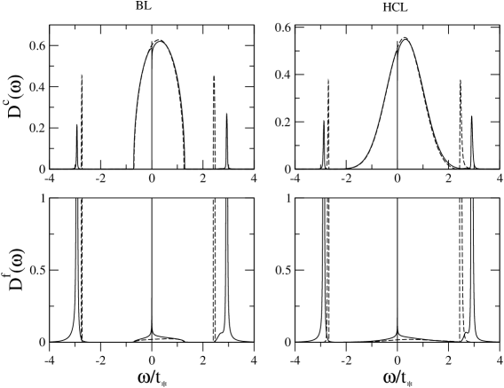
Figure 2: All scales view of LMA $c$- and $f$-electron spectra (solid lines): $D^{c}({\omega})$ and $D^{f}({\omega})$ vs ${\omega}$ $(\equiv{\omega}/t_{*})$, for Bethe lattice (left panels) and hypercubic lattice (right panels). For $U\simeq 5.1$ $(x=\tfrac{1}{2}U|\mu|=2.5)$, $V^{2}=0.2$, ${\epsilon}_{c}=0.3$ and $\eta=1-2|{\epsilon}_{f}|/U=0$. Corresponding MF spectra are also shown (dashed lines).

For obvious physical reasons the primary interest in the PAM resides both in the strongly correlated Kondo lattice regime, and on energies on the order of the coherence scale ${\omega}_{L}=ZV^{2}$ and (essentially arbitrary) multiples thereof. We begin however with an overview on all energy scales — encompassing ‘band scales’ ${\omega}\sim{\cal{O}}(1)$ ($1\equiv t_{*})$ and energies $\omega\sim\epsilon_{f}$ or $\epsilon_{f}+U$ characteristic of the $f$-electron Hubbard satellites. In contrast to the low-energy sector, dynamics here will naturally be non-universal: dependent on essentially all bare material/model parameters, and lattice specific. An overview is nonetheless instructive, showing clearly the roles of asymmetry (in both the conduction band and $f$-levels), and of the lattice type, as well as qualitative effects of depleting the conduction band filling. In addition, it enables broad comparison both to dynamics arising at the crude level of pure MF (§4.2) and to corresponding results for the Anderson impurity model ($\S 4.5$).

Figs.2 and 3 show spectra typical of metallic heavy fermion behaviour in strong coupling: $U\simeq 5.1$ ($x=\tfrac{1}{2}U|\mu|\\ =2.5$), $V^{2}=0.2$ and ${\epsilon}_{c}=0.3$. In Fig.2, $\eta=1+2{\epsilon}_{f}/U=0$ is taken — corresponding to symmetric $f$-levels ${\epsilon}_{f}=-\tfrac{U}{2}$, but with asymmetry in the conduction band (${\epsilon}_{c}\neq 0$). To illustrate the effects of the lattice, the $c$- and $f$-electron spectra are each shown for both the hypercubic lattice (HCL) and Bethe lattice (BL). In either case the $f$-level charge $n_{f}\simeq 0.99$. The conduction band fillings, likewise determined from spectral integration, differ little for the two lattices, $n_{c}\simeq 0.64$ (BL) and $0.69$ (HCL) (each being within $\sim 2\%$ of the asymptotic strong coupling result Eq.(3.13) for $n_{c}$).

The overwhelming intensity of the $f$-spectra shown in Fig.2 is naturally in the Hubbard satellites, well separated from the band scales $\omega\sim{\cal{O}}(1)$ (and in consequence sharply distributed). Their peak maxima are symmetrically positioned about the Fermi level — reflecting the fact that the $f$-levels themselves are symmetric ($\eta=0$) — and largely unaffected by the presence of asymmetry in the conduction band. The most important feature of the $f$-spectra is of course the well known many-body resonance at low energies. Its rich structure, considered in detail in §5.3, is naturally not resolved here. What is however evident from Fig.2 is the relative unimportance of the host lattice in determining the $f$-spectra on the all scales level shown. This is in contrast to the local conduction electron spectra (top panels, Fig.2). Here, aside from weakly remnant Hubbard satellites whose intensity diminishes steadily with increasing $U$, the $c$-spectra are clearly dominated by the asymmetrically distributed envelope of the free ($V=0$) conduction band spectrum, semi-elliptic for the BL and Gaussian for the HCL. As mentioned at the end of §3 this is physically natural, reflecting that in the strongly correlated regime the conduction band is very weakly coupled to the $f$-levels; albeit that such coupling is of course the key feature of the problem on low energy scales, where it leads to many-body structure in the $D^{c}({\omega})$ (again barely visible on the scales shown). In Fig.3, shown for the HCL with $\eta=0.4$, there is now particle-hole asymmetry in the $f$-levels as well as in the conduction band; producing the additional spectral signature of asymmetry in the positions of the Hubbard satellites, but otherwise little change in broad terms.

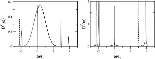
Figure 3: Local $c$- and $f$-electron spectra for the HCL: $D^{c}({\omega})$ and $D^{f}({\omega})$ vs ${\omega}$, shown for $\eta=1-2|{\epsilon}_{f}|/U=0.4$ with remaining parameters as in Fig.2. Dashed lines: corresponding MF spectra.

Figs.2 and 3 also show direct comparison to the corresponding spectra at pure mean-field level (dashed lines). At first sight, and on the all scales level shown, these appear to provide a reasonable first approximation to dynamics. That is not of course the case on the all important low-energy scales that dominate the physics of the PAM in strong coupling: MF clearly lacks any hint of the many-body resonance in the $f$-spectra and its counterpart in $D^{c}({\omega})$ — unsurprisingly given the absence of correlated electron dynamics at this crude level — and in fact for $D^{f}({\omega})$ is seen to be qualitatively deficient for essentially all $|{\omega}|\lesssim 1$. For the $c$-electron spectra however, and again excepting the lowest energies, MF is qualitatively reasonable, reducing in strong coupling to precisely the free conduction band spectrum (as is readily shown directly from Eqs.(4.11)). In addition, MF also captures qualitatively the dominant Hubbard satellites in the $f$-electron spectra; albeit that many-body broadening effects, arising from the spin-flip dynamics included in the LMA, lead both to a broadening and slight shift of the satellites (which can be understood quantitatively in terms of the ${\omega}$-dependence of the dynamical self-energies $\Sigma_{\sigma}({\omega})$, although we do not pursue that further here).

We consider now the qualitative effect of depleting the conduction band filling $n_{c}$, obtained by increasing ${\epsilon}_{c}$ significantly. Fig.4 shows HCL spectra for ${\epsilon}_{c}=1.5$, $U\simeq 7$ ($x=3.5$), $\eta=0.8$ and $V^{2}=1.25$; for which the resultant $n_{c}\simeq 0.2$ (and $n_{f}\simeq 0.85$). Save for the large $\epsilon_{c}$ the remaining parameters have no special significance, and the large $V^{2}$ has simply been chosen so that the resultant low-energy scale ${\omega}_{L}$ (discussed in detail in §5.2) is not so small as to be in effect invisible in the figure shown. Depleting $n_{c}$ in this way has a marked effect on the conduction electron spectra. In contrast to Figs.2,3 for ${\epsilon}_{c}=0.3$ — where the low-energy ‘antiresonance’ in $D^{c}({\omega})$ is carved out of the free conduction band envelope — Fig.4 shows that the low-$n_{c}$ conduction spectrum now contains a sharp low-energy resonance lying in the tail of the free conduction band envelope, akin to that appearing ubiquitously in the local $f$-spectra. The essential origin of the resonance is readily seen from the quasiparticle behaviour discussed in §3: from the quasiparticle $D^{c}({\omega})$ Eq.(3.11a), the Fermi level $D^{c}({\omega}=0)\sim\rho_{0}(-{\epsilon}_{c}+1/\tilde{{\epsilon}}_{f}^{*})$ (with $\tilde{{\epsilon}}^{*}_{f}={\epsilon}_{f}^{*}/V^{2}$ and ${\epsilon}_{f}^{*}$ the renormalized level); while for large ${\epsilon}_{c}=|{\epsilon}_{c}|$, Eq.(3.12) shows that $-{\epsilon}_{c}+1/\tilde{{\epsilon}}^{*}_{f}\rightarrow 0$ as $n_{f}\rightarrow 1$. In consequence, $D^{c}({\omega}=0)\sim\rho_{0}({\omega}=0)$ is effectively pinned at the Fermi level to its free lattice limit (with $\rho_{0}(0)=1/\sqrt{\pi}$ for the HCL marked explicitly on Fig.4); and the width of the resultant resonance is ${\cal{O}}({\omega}_{L})$, as again follows from the quasiparticle $D^{c}({\omega})$, Eq.(3.11a). The low-energy resonance arising for low $n_{c}$ in the $c$-electron spectrum thus reflects directly the Fermi liquid nature of the ground state.

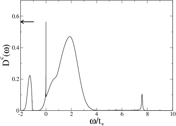
Figure 4: Depleting the conduction band: $D^{c}({\omega})$ vs ${\omega}$ for the HCL with ${\epsilon}_{c}=1.5$, $U\simeq 7$ ($x=3.5$), $\eta=0.8$ and $V^{2}=1.25$, corresponding to $n_{c}\simeq 0.2$. The conduction band spectrum now shows a sharp resonance in the vicinity of the Fermi level ${\omega}=0$ (cf Figs.2,3) as explained in text; $\rho_{0}({\omega}=0)=1/\sqrt{\pi}$ is indicated by an arrow.

In Fig.5, comparison is made between an $f$-electron spectrum for the PAM for the HCL (solid line) and its counterpart for the single-impurity Anderson model (dash-ed line); the bare parameters chosen for illustration being $\eta=0$ (symmetric $f$-level(s)), $U\simeq 1.3$ ($x=0.5$) and $V^{2}=0.2$, ${\epsilon}_{c}=0.3$ (corresponding to a hybridization strength, Eq.(4.21), of $\pi\Delta_{0}=(\pi V)^{2}\rho_{0}(-{\epsilon}_{c})\simeq 1$). The spectra, specifically $\pi\Delta_{0}D^{f}({\omega})$, are compared on the all scales level in the main figure (vs ${\omega}\equiv{\omega}/t_{*}$); and on the low-energy resonance scale in the inset. The main figure shows in addition the impurity spectrum for ${\epsilon}_{c}=0$ (with the same parameters otherwise), which is of course the fully particle-hole symmetric AIM. The first point to note here is obvious: excepting the low-energy sector, the PAM and corresponding AIM spectra are qualitatively very similar on the ‘all scales’ level (which is not specific to the particular parameter set employed). This general characteristic is in agreement with results from a numerical renormalization group (NRG) study of the PAM and AIM [8], see e.g. Figs.1,4,6 of [8]. Note further, in comparison to the fully particle-hole symmetric AIM (dotted line), that for the moderate value of $U$ chosen in Fig.5 the asymmetry in the conduction band (${\epsilon}_{c}\neq 0$) shows up weakly in the Hubbard satellites, both in their intensities and maxima (which are not quite symmetrically positioned about the Fermi level).

It is naturally in the low-energy behaviour that the PAM and AIM spectra differ significantly, as evident in the inset to Fig.5. In particular, for the PAM the lattice coherence generates a pseudogap above the Fermi level, as indeed expected from the quasiparticle behaviour of $D^{f}({\omega})$, Eq.(3.11b) (albeit that the relative weakness of the pseudogap here reflects the moderate $U$ considered, see §5.3). However even at low energies one does not learn much from comparison of PAM and AIM dynamics on an absolute scale, e.g. vs ${\omega}\equiv{\omega}/t_{*}$, and for a given set of bare parameters $\{{\epsilon}_{c},V^{2},U,\eta\}$. For the parameters chosen in Fig.5, it so happens that the low-energy scales for the PAM and AIM are very similar (with quasiparticle weights $Z\approx 0.1$). But that is not generically so: as discussed in §5.2 the PAM lattice coherence scale and the Kondo scale for the AIM will in general be quite different for given bare parameters [8,23] (they are after all physically distinct models), whence comparison of the two on an absolute scale is barely informative. What is required by contrast — particularly in strong coupling where there is a pristine separation between asymptotically vanishing low-energy scale(s) and non-universal scales such as $\Delta_{0}$, $t_{*}\equiv 1$ or $U$ — is comparison of the universal scaling behaviour of the two models; in which the dependence of the respective low-energy scales on bare parameters is thereby eliminated and the underlying scaling behaviour exposed. This we believe is the most convincing (and possibly only) way to establish a connection between the high-energy scaling behaviour of the PAM/KLM and underlying single-impurity physics. That key issue is considered in §5.3.

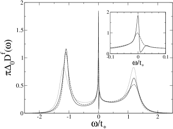
Figure 5: All scales comparison of local $f$-electron spectra for the PAM and Anderson impurity model: $\pi\Delta_{0}D^{f}({\omega})$ vs ${\omega}\equiv{\omega}/t_{*}$ (with $\Delta_{0}=\pi V^{2}\rho_{0}(-{\epsilon}_{c})$); for ${\epsilon}_{c}=0.3$, $U\simeq 1.3(x=0.5),V^{2}=0.2$ and $\eta=0$. Solid line: PAM. Dashed line: AIM. Inset: comparison on the resonance scales. The impurity spectrum for ${\epsilon}_{c}=0$ is also shown on the main figure (dotted line, the particle-hole symmetric AIM).

5.2 Low-energy scale

We first consider briefly how the low-energy coherence scale for the PAM, ${\omega}_{L}=ZV^{2}$ (Eq.(3.10)), is found within the LMA to depend on the bare/material parameters $({\epsilon}_{c},\\ V^{2},U,\eta)$ in the strong coupling Kondo lattice regime where $n_{f}\rightarrow 1$; and how it compares to the Kondo scale for the corresponding AIM, ${\omega}_{K}\equiv Z_{imp}V^{2}$ (with $Z_{imp}$ denoting the quasiparticle weight for the single-impurity model). The scales ${\omega}_{L}$ and ${\omega}_{K}$ are indeed found to be exponentially small in strong coupling (as opposed to algebraically small, such as arises using perturbation theory in $U$ or variants thereof such as modified (iterated) perturbation theory [14-17]); leading thereby to the clean scale-separation that is a prerequisite to the scaling considerations of §5.3. The essential findings here, discussed below, agree with the NRG study of [8] and results obtained from the large-$N$/slave boson mean-field (SBMF) approximation [23]: (a) That the scales ${\omega}_{L}$ and ${\omega}_{K}$ are found to have the same exponential dependence on the bare parameters, but (b) depend very differently on the conduction band filling $n_{c}$; the lattice scale ${\omega}_{L}$ being enhanced relative to its single-impurity counterpart as $n_{c}\rightarrow 1$, but strongly diminished for low $n_{c}$.

The material dependence of the AIM Kondo scale ${\omega}_{K}(\propto{\omega}_{m})$ arising within the LMA can be obtained analytically in strong coupling by direct analysis of the symmetry restoration condition Eq.(4.13). That was considered explicitly in [27] for the case of a general impurity (with $f$-level asymmetry embodied as usual in $\eta\equiv 1-2\tfrac{|{\epsilon}_{f}|}{U}$), but a symmetric host band. It is straightforward to extend the analysis of [27] to include the ${\omega}$-dependence of the hybridization $\Delta({\omega})$ arising from an asymmetric host conduction band (which as anticipated in §4.5 does not affect the final answer). Noting that the AIM hybridization strength is given by $\Delta_{0}=\pi V^{2}\rho_{0}(-{\epsilon}_{c})$ (Eq.(4.21)), this yields

$${\omega}_{K}\propto~{}\exp\left(-\frac{U}{8V^{2}\rho_{0}(-{\epsilon}_{c})}\frac{(1-\eta^{2})}{f(\eta^{2})}\right)$$ (5.1)

(with the proportionality determined simply by a high-energy cutoff [27]); where $f(\eta^{2})=\tfrac{1}{2}[1+\sqrt{(1-\eta^{2})}]$ ($\in[1,\tfrac{1}{2}]$ for asymmetries $|\eta|\in[0,1]$ relevant to the Kondo regime). The exchange coupling $J$ for the corresponding Kondo model, obtained from the AIM in strong coupling by a Schrieffer-Wolff transformation [2], is given by $J=V^{2}[\tfrac{1}{|{\epsilon}_{f}|}+\tfrac{1}{U-|{\epsilon}_{f}|}]\equiv 4V^{2}/[U(1-\eta^{2})]$; whence Eq.(5.1) is equivalently ${\omega}_{K}\propto\exp(-1/[2\rho_{0}(-{\epsilon}_{c})Jf])$. As pointed out in [27] the exponent here differs in general by the factor $f(\eta^{2})$ from the exact result for the Kondo model, being as such exact only for the symmetric case where $\eta=0$ (although note that $f$ is slowly varying in $\eta$, lying e.g. within 10$\%$ of unity for $\eta<0.6$). That notwithstanding we regard recovery of an exponentially small Kondo scale, close to the exact result in an obvious sense, as non-trivial; and add that provided the scale is indeed exponentially small, so that a clean separation of low (universal) and non-universal energies arises, its precise dependence on the bare parameters is in essence irrelevant to the issue of scaling in terms of ${\omega}/{\omega}_{K}$ (as seen in [27] for the AIM itself).

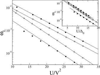
Figure 6: PAM coherence scale ${\omega}_{L}$ on a log-scale vs $U/V^{2}$; for the BL with $\eta=0$, ${\epsilon}_{c}=0.1$ (solid circles) and ${\epsilon}_{c}=0.6$ (solid squares). Comparison is made to corresponding results for the AIM Kondo scale ${\omega}_{K}$: ${\epsilon}_{c}=0.1$ (open circles) and ${\epsilon}_{c}=0.6$ (open squares). ${\omega}_{L}$ is enhanced relative to ${\omega}_{K}$ for ${\epsilon}_{c}=0.1$ but diminished for ${\epsilon}_{c}=0.6$ (see also Fig.7). The straight lines indicate the exponents given by Eq.(5.1), found for both models. Inset: same results now shown vs $U/\Delta_{0}$ (with $\Delta_{0}=\pi V^{2}\rho_{0}(-{\epsilon}_{c})$). The strong coupling gradients are then common for different ${\epsilon}_{c}$, as implied by Eq.(5.1).

For the PAM the coherence scale ${\omega}_{L}$ is likewise obtained from solution of the symmetry restoration condition Eq.(4.13), in this case numerically following the procedure detailed in §4.4 (and with ${\omega}_{L}$ found to be proportional to the spin-flip scale ${\omega}_{m}$ as noted in §4.4). In the strong coupling Kondo lattice regime ${\omega}_{L}$ is again found to be exponentially small, with its exponential dependence on the bare parameters the same as ${\omega}_{K}$ for the AIM. This is illustrated in Fig.6 (for the BL) where, with $\eta=0$ and for ${\epsilon}_{c}=0.1$ and $0.6$, the resultant ${\omega}_{L}$ is plotted on a logarithmic scale vs $U/V^{2}$; and compared to the counterpart ${\omega}_{K}$ results for the AIM itself. For given ${\epsilon}_{c}$ the asymptotic PAM and AIM curves are parallel, indeed indicating common $U/V^{2}$-dependence for the exponents of the two scales. When plotted vs $U/V^{2}$ as in the main figure, the slopes for different ${\epsilon}_{c}$ clearly differ; but when shown vs $U/\Delta_{0}=U/(\pi V^{2}\rho_{0}(-\epsilon_{c}))$ as in the inset to Fig.6, the gradients for different $\epsilon_{c}$ are now common in strong coupling, as implied by the exponential dependence of Eq.(5.1). The dependence of the exponents on the $f$-level asymmetry, as in Eq.(5.1), may likewise be verified by varying $\eta$. And the same exponential dependence, Eq.(5.1), is found whether the BL or HCL is considered.

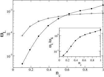
Figure 7: PAM coherence scale ${\omega}_{L}$ vs $n_{c}$, for the BL with $U/V^{2}=23$ and $\eta=0$ (solid circles), compared to the AIM Kondo scale ${\omega}_{K}$ (open circles). Inset: ${\omega}_{L}/{\omega}_{K}$ vs $n_{c}$.

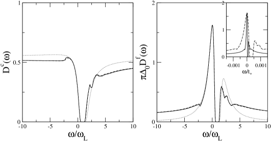
Figure 8: Universal spectral scaling. $D^{c}({\omega})$ and $\pi\Delta_{0}D^{f}({\omega})$ vs ${\omega}^{\prime}={\omega}/{\omega}_{L}$ for the HCL with ${\epsilon}_{c}=0.2$ and $\eta=0$. The spectra for $U\simeq 5.1$ (dashed line) and $U\simeq 6.6$ (solid line) collapse to a common scaling form as a function of ${\omega}/{\omega}_{L}$. Inset: corresponding $f$-spectra shown by contrast on an absolute scale, vs $\omega/t_{*}$. The main figures also show the asymptotic low-$|{\omega}^{\prime}|$ quasiparticle spectra (Eqs.(3.11)), dotted lines; to which the full scaling spectra reduce for $|{\omega}^{\prime}|\lesssim 1$.

While the exponents of the scales ${\omega}_{L}$ and ${\omega}_{K}$ have the same dependence on bare parameters, their dependence on the conduction band filling $n_{c}$ (which itself is determined solely by ${\epsilon}_{c}$ in strong coupling, see Eq.(3.13)) is quite distinct for the two models. This is evident already in Fig.6 but seen more clearly in Fig.7 where, for $U/V^{2}=23$ (and $\eta=0$) we show ${\omega}_{L}$ and ${\omega}_{K}$ vs $n_{c}$ (their ratio being shown in the inset). For $n_{c}\rightarrow 1$, ${\omega}_{L}/{\omega}_{K}=F(n_{c})>1$ and the lattice scale is enhanced over its AIM counterpart; while with decreasing ${\epsilon}_{c}$ (and hence $n_{c}$) ${\omega}_{L}$ diminishes progressively in comparison to ${\omega}_{K}$, such that $F(n_{c})\rightarrow 0$ as $n_{c}\rightarrow 0$. As noted above this general behaviour is in agreement with NRG [8] and SBMF results [23]. It is by contrast quite distinct from results arising from a Gutzwiller variational treatment [24] in which the lattice scale is always enhanced over its AIM counterpart; or from approaches based on lattice extensions of the non-crossing approximation (NCA) [18,19] in which the lattice scale, while in general moderately enhanced compared to $\omega_{K}$, is essentially equivalent to the AIM scale.

5.3 Scaling

The preceding discussion of how ${\omega}_{L}$ and ${\omega}_{K}$ for the two different models depend on bare parameters has been included in part because of the interest it has hitherto attracted in the literature. As noted earlier however we regard this matter as quite subsidiary in comparison to the strong coupling scaling behaviour of the lattice model itself, as now considered.

First we show that in the Kondo lattice regime the LMA indeed leads to universal scaling of single-particle dynamics in terms of ${\omega}/{\omega}_{L}$, for fixed ${\epsilon}_{c}$ and $\eta$. This is illustrated for the hypercubic lattice in Fig.8, for ${\epsilon}_{c}=0.2$ and $\eta=0$. The inset to the figure shows the $f$-electron spectrum $\pi\Delta_{0}D^{f}({\omega})$ on an absolute scale, i.e. vs ${\omega}$ ($\equiv{\omega}/t_{*}$), for $V^{2}=0.2$ and two different interaction strengths, $U\simeq 5.1$ ($x=2.5$) and $U\simeq 6.6$ ($x=3.25$). In either case the resultant conduction band filling $n_{c}\simeq 0.78$, in agreement with the asymptotic result Eq.(3.13) which shows that $n_{c}$ is determined by ${\epsilon}_{c}$ alone; and likewise $n_{f}\simeq 0.99$. As seen from the inset the two spectra are quite distinct on an absolute scale and dependent on the bare model parameters, reflecting the exponential diminution of the coherence scale $\omega_{L}$ with increasing $U/V^{2}$ as in §5.2 above. The main part of Fig.8 by contrast shows both $\pi\Delta_{0}D^{f}({\omega})$ and the corresponding conduction spectrum $D^{c}({\omega})$, now vs ${\omega}^{\prime}={\omega}/{\omega}_{L}$, from which collapse to common scaling forms and hence universality is clear. While scaling has been demonstrated here by considering fixed $V^{2}$ upon increasing $U$ in the KL regime, it is as expected dependent solely on the ratio $U/V^{2}$ (the same scaling spectrum arising for fixed $U$ upon decreasing $V^{2}$).

As discussed in §3, adiabatic continuity to the non-interacting limit requires that for sufficiently low ${\omega}^{\prime}$ the scaling spectra should reduce to the quasiparticle forms Eq.(3.11). That this behaviour is indeed recovered correctly by the LMA is also seen in Fig.8, where the resultant quasiparticle spectra are shown for comparison (dotted lines, as given by Eq.(3.11) with $\tilde{{\epsilon}}^{*}_{f}\equiv\tilde{{\epsilon}}^{*}_{f}({\epsilon}_{c})$ obtained from Eq.(3.12) with $n_{f}=1$): in the vicinity of the Fermi level (${\omega}^{\prime}=0$), and up to $|{\omega}^{\prime}|\simeq 1$ or so, agreement with the quasiparticle behaviour is essentially perfect. For larger $|{\omega}^{\prime}|$ by contrast, an evident departure from this simple low-${\omega}^{\prime}$ asymptotic behaviour sets in; in particular, the quasiparticle $f$-electron spectra for large $|{\omega}^{\prime}|$ are seen to decay much more rapidly ($\sim 1/|{\omega}^{\prime}|^{2}$) than the full LMA results, which show instead slowly decaying spectral tails. The latter, which as shown below decay logarithmically slowly, are a key feature of dynamics (see Figs.11-13); reflecting genuine many-body scattering/lifetime effects, setting in for $|{\omega}^{\prime}|\gtrsim 1-10$ and dominating the scaling spectra (as well as transport properties on corresponding temperature scales, see e.g. [34,35]). Here we note in passing that scaling spectra arising from a SBMF approximation are just the quasiparticle forms themselves, and are evidently deficient except for the lowest energy scales; and similarly that dynamics arising from modified (iterated) perturbation theory [16,17] amount to little more than quasiparticle form, and similarly lack non-trivial high-energy scaling behaviour [35]. We also add that the spectral substructure seen in Fig.8 just above the upper edge of the gap is not a numerical artefact, and using the LMA self-energies can in fact be understood physically in terms of correlated ‘strings’ of $f$-electron spin-flips on distinct lattice sites. It is however destroyed thermally on temperature scales which are a small fraction of ${\omega}_{L}$ itself (as will be shown in subsequent work), and as such is but a minor feature of dynamics that we do not pursue further here.

The spectra shown in Fig.8 display an evident gap lying slightly above the Fermi level (strictly a pseudogap for the HCL), as found also in approaches based on lattice extensions of the NCA [18-20]. That such behaviour arises is to be expected, for it occurs likewise in the quasiparticle spectra Eqs.(3.11) (see also the discussion at the end of §2.1). Note however that this gap become ‘fully developed’ only in the strong coupling Kondo lattice regime; for weaker interaction strengths outside the scaling spectrum it is by contrast incompletely formed and evident only as a weaker pseudogap, as seen clearly e.g. in Fig.5. But for sufficiently strong coupling we find that a well developed gap always arises (as the quasiparticle forms would suggest). Such behaviour is also found in recent NRG calculations [8] for $n_{c}\sim 1$, but not for significantly lower conduction band fillings – see e.g. Fig.7 of [8] for $D^{c}({\omega})$ with $n_{c}=0.6$ where, by contrast, only weaker pseudogap behaviour is evident. However the spectrum e.g. in Fig.7 of [8] is clearly not close to strong coupling behaviour; as evidenced both from the fact that the $D^{c}({\omega})$ shown there departs significantly from the free conduction band envelope well into non-universal energy scales ${\cal{O}}(t_{*})$, and because the quoted $n_{c}=0.6$ is far from its asymptotic strong coupling value of $n_{c}=0.48$ (from Eq.(3.13) above) for the bare parameters specified. Further resolution of this matter is clearly required, but we suspect that the parameter regime considered e.g. in Figs.6,7 of [8] was not sufficiently strong coupling to uncover a well developed spectral gap.

The scaling spectra shown in Fig.8 refer specifically to ‘LMAI’ as detailed in §4.3, on which we focus in this paper. In Fig.9 however we compare the resultant $f$-electron scaling spectra $\pi\Delta_{0}D^{f}(\omega)$ with those arising from ‘LMAII’, where (see §4.3) the polarization propagators entering the LMA self-energies are further renormalized in terms of the host/medium propagators $\{\tilde{\cal{G}}_{\sigma}({\omega})\}$; again for the HCL with ${\epsilon}_{c}=0.2$ and $\eta=0$. The inset shows the LMAI/II comparison out to ${\omega}^{\prime}=10$, while the main figure extends to much larger scales. And the two spectra are seen to be essentially coincident on all ${\omega}^{\prime}$ scales (as they ought to be if the LMA captures adequately the scaling spectrum).

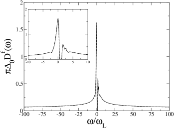
Figure 9: Comparison of $f$-electron scaling spectra arising from LMAI (solid line) and LMAII (dashed line), as explained in text: $\pi\Delta_{0}D^{f}(\omega)$ vs ${\omega}/{\omega}_{L}$ for ${\epsilon}_{c}=0.2$ and $\eta=0$. The two levels of LMA yield essentially coincident scaling spectra.

Fig.8 above illustrates that universal spectral scaling, independent of $U$ and $V^{2}$, arises for fixed ${\epsilon}_{c}$ and $\eta$ which embody respectively asymmetry in the conduction band and $f$-levels. This we find to be quite general: $D^{c}({\omega})$ and/or $\pi\Delta_{0}D^{f}(\omega)$ exhibit scaling as an entire function of ${\omega}^{\prime}={\omega}/{\omega}_{L}$ only for fixed $({\epsilon}_{c},\eta)$, i.e. distinct scaling spectra arise for different $({\epsilon}_{c},\eta)$. Much more subtly however, the ${\epsilon}_{c}$- and $\eta$-dependences of the scaling spectra depend upon the ${\omega}^{\prime}$-regimes considered, as now explained. We begin with the simple case of low-${\omega}^{\prime}$. As pointed out in §3, the quasiparticle spectra Eq.(3.11) imply that — in their ${\omega}^{\prime}$-regime of validity — the scaling spectra should actually be independent of the $f$-level asymmetry $\eta$. That this is recovered within the LMA is seen in Fig.10 for the HCL where, for fixed ${\epsilon}_{c}=0.3$, the $f$-electron scaling spectra $\pi\Delta_{0}D^{f}({\omega})$ are shown for three different $f$-asymmetries $\eta=0,0.2,0.4$. For $|{\omega}^{\prime}|\lesssim 1$, the regime where the quasiparticle forms hold, the LMA scaling spectra are indeed seen to be independent of $\eta$; while for larger-$|{\omega}^{\prime}|$ by contrast, an $\eta$-dependence to the spectra is evident (and discussed further below). Likewise, for $|{\omega}^{\prime}|\lesssim 1$, the quasiparticle forms Eq.(3.11) show that the scaling spectra depend explicitly on ${\epsilon}_{c}$, as well as on the underlying lattice itself (embodied in the specific form for $\rho_{0}({\omega})$).

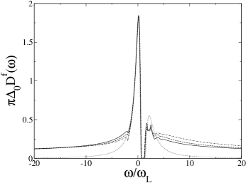
Figure 10: Independence of the low-$|{\omega}^{\prime}|$ scaling spectra on the $f$-level asymmetry, $\eta$. For the HCL with fixed ${\epsilon}_{c}=0.3$, $\pi\Delta_{0}D^{f}({\omega})$ vs ${\omega}^{\prime}={\omega}/{\omega}_{L}$ is shown for $\eta=0$ (solid line), $0.2$ (dashed line) and $0.4$ (point dash). The limiting low-$|{\omega}^{\prime}|$ quasiparticle form is again shown for comparison (dotted line).

But what of higher energies in the scaling spectra? Here as we now show the low-${\omega}^{\prime}$ situation above is reversed: the high-energy scaling behaviour of the $f$-electron spectrum is dependent on the asymmetry $\eta$, but independent of both ${\epsilon}_{c}$ and the underlying host lattice; the latter in turn being intimately related to the emergence of effective single-impurity physics in the high-energy scaling behaviour of the PAM.

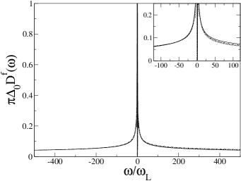
Figure 11: $\pi\Delta_{0}D^{f}({\omega})$ vs ${\omega}^{\prime}={\omega}/{\omega}_{L}$ for the HCL up to $|{\omega}^{\prime}|=500$, for $\eta=0$ and three different ${\epsilon}_{c}=0$ (solid line), $0.3$ (dashed line) and $0.5$ (point dash); obtained explicitly for $U\simeq 6.6$ and $V^{2}=0.2$. Inset: $\pi\Delta_{0}D^{f}({\omega})$ vs ${\omega}^{\prime}$ for fixed ${\epsilon}_{c}=0.3$ with increasing interaction strength $x=\tfrac{1}{2}U|\mu|=2.0$ (solid line), $2.5$ (double point dash) and $3.25$ (long dash); the true scaling limit is also indicated (dotted line). Full discussion in text.

To see this, Fig.11 (for the HCL) shows $\pi\Delta_{0}D^{f}({\omega})$ vs ${\omega}^{\prime}={\omega}/{\omega}_{L}$ up to $|{\omega}^{\prime}|=500$, for $\eta=0$ and three different ${\epsilon}_{c}=0,0.3,0.5$ (progressively diminishing conduction band filling $n_{c}$); the particular results shown having been obtained explicitly for $U\simeq 6.6$ ($x=\tfrac{1}{2}U|\mu|=3.25$) and $V^{2}=0.2$. Looking at the negative-${\omega}^{\prime}$ side in particular, it is clear that the slowly decaying spectral ‘tails’ are indeed asymptotically common for the different ${\epsilon}_{c}$’s. On the positive-${\omega}^{\prime}$ side there might appear from the figure to be a residual weak dependence of the spectral tails on ${\epsilon}_{c}$. That however is simply a reflection of the natural fact that the value of $U/V^{2}$ required to reach the full asymptotic scaling spectra is dependent upon ${\epsilon}_{c}$. This is illustrated further in the inset to Fig.11, which for fixed ${\epsilon}_{c}=0.3$ shows (on an expanded scale) the evolution of the scaling spectrum with increasing interaction strength: $x=2.0,2.5$ and $3.25$. Looking at the positive ${\omega}^{\prime}$ side one sees that the true scaling limit (dotted line) is steadily approached upon increasing the interaction strength, but not reached until a $U$ somewhat in excess of $\simeq 6.6$ ($x=3.25$). On the negative ${\omega}^{\prime}$ side by contrast, the scaling limit is already reached by $x=2.5$ ($U\simeq 5.1$) and does not change with further increasing interaction strength. This is why the ${\epsilon}_{c}$-independence of the spectral tails is clearly evident only on the ${\omega}^{\prime}<0$ side of the main figure; upon increasing $U$ however both sides of the scaling spectra show this behaviour.

What then is the functional form of the large-$|{\omega}^{\prime}|$ spectral tails? On physical grounds one expects that on sufficiently high energy and/or temperature scales, the $f$-electrons in the Kondo lattice regime of the PAM should be screened in an essentially incoherent single-impurity fashion; and thus that effective single-impurity physics should arise in the lattice model at high energies, quite distinct from the effects of lattice coherence evident on low-energy scales ${\omega}/{\omega}_{L}\sim{\cal{O}}(1)$. For the AIM itself the spectral tails of the local impurity scaling spectrum $D_{imp}(\omega)$ can be obtained analytically within the LMA [27,28]; being given by

$$\pi\Delta_{0}D_{imp}({\omega})\sim\frac{1}{2}\left(\frac{1}{[\tfrac{4}{\pi}\ln(c|\tilde{{\omega}}|)]^{2}+1}+\frac{5}{[\tfrac{4}{\pi}\ln(c|\tilde{{\omega}}|)]^{2}+25}\right)$$ (5.2)

(shown explicitly for $\eta=0$) where $\tilde{{\omega}}={\omega}/{\omega}_{K}$ with ${\omega}_{K}$ the Kondo scale for the AIM discussed in §5.2, and $c$ a pure constant ${\cal{O}}(1)$. For $\tilde{\omega}\gtrsim 5-10$ or so, Eq.(5.2) is known [28] to describe quantitatively the spectral tails arising from NRG calculations; the exact high energy scaling asymptote $\pi\Delta_{0}D_{imp}({\omega})\sim 3\pi^{2}/[16\ln^{2}({\omega}/{\omega}_{K})]$ being recovered in particular. If effective single-impurity behaviour arises in the PAM on energy scales encompassed by the ${\omega}^{\prime}$-scaling regime, then the spectral tails thereof should have the same scaling form as for the AIM, i.e. should be given by

$$\pi\Delta_{0}D^{f}({\omega})\sim\frac{1}{2}\left(\frac{1}{[\tfrac{4}{\pi}\ln(a|{\omega}^{\prime}|)]^{2}+1}+\frac{5}{[\tfrac{4}{\pi}\ln(a|{\omega}^{\prime}|)]^{2}+25}\right)$$ (5.3)

with ${\omega}^{\prime}={\omega}/{\omega}_{L}$ and $a$ a constant ${\cal{O}}(1)$. Note that such comparison requires neither a knowledge of how the low-energy scales for the two distinct models (${\omega}_{L}$ and ${\omega}_{K}$) depend on the bare material parameters, nor any assumption that the Kondo scale for the AIM itself is at all relevant to the PAM; points to which we return again in §5.4.

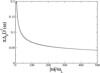
Figure 12: Effective single-impurity physics arising in the PAM scaling spectra at high energies, as explained in the text. The PAM $\pi\Delta_{0}D^{f}({\omega})$ vs $|{\omega}|/{\omega}_{L}$ on an expanded vertical scale, for $\eta=0$ and ${\epsilon}_{c}=0$ (solid line), $0.3$ (dashed line) and $0.5$ (double point dash); compared to the scaling form Eq.(5.3) (dotted line, barely distinguishable in the figure).

Eq.(5.3) indeed describes the tail behaviour of the PAM scaling spectra, and as such establishes the connection to effective single-impurity behaviour at high energies. This is shown explicitly in Fig.12 where, again for $\eta=0$ and ${\epsilon}_{c}=0,0.3$ and $0.5$ (as in Fig.11), $\pi\Delta_{0}D^{f}({\omega})$ is shown vs $\omega^{\prime}$ on an expanded vertical scale, and compared to Eq.(5.3) (with the constant $a\simeq 0.55$ determined numerically). That form is clearly seen to hold asymptotically for the different ${\epsilon}_{c}$’s; and even for lower ${\omega}^{\prime}$ the spectra display only a very weak dependence on ${\epsilon}_{c}$. Neither is it lattice dependent, the same asymptotic tail behaviour being found to arise whether the HCL or BL is considered; naturally so, for effective single-impurity scaling physics should be independent of the ‘host’ lattice.

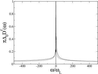
Figure 13: $f$-electron scaling spectra $\pi\Delta_{0}D^{f}({\omega})$ vs ${\omega}^{\prime}={\omega}/{\omega}_{L}$, for $\eta=0$ (solid line) and $\eta=0.3$ (dashed line); shown explicitly for ${\epsilon}_{c}=0$ (the scaling spectra at low-${\omega}^{\prime}$ depend upon ${\epsilon}_{c}$, see text).

While the discussion above has focused on varying ${\epsilon}_{c}$ (and hence $n_{c}$) for symmetric $f$-levels $\eta=0$, the behaviour found is quite general. For fixed $\eta\neq 0$ the high-energy PAM scaling spectrum is likewise independent of both ${\epsilon}_{c}$ and the lattice type; and is again found to have precisely the same scaling form as its counterpart for the AIM (the generalisation of Eq.(5.2) to finite-$\eta$, specifically Eq.(5.5) of [27]). As for the AIM [27] the resultant $f$-electron scaling spectra are now $\eta$-dependent, as illustrated in Fig.13 where $\pi\Delta_{0}D^{f}(\omega)$ is compared for $\eta=0$ and $0.3$ (and is shown specifically for ${\epsilon}_{c}=0$, bearing in mind that the spectra at low-$\omega^{\prime}$ depend on ${\epsilon}_{c}$ as discussed above). The $\eta$-dependence of the spectral tails is clearly evident, albeit rather weakly so for positive ${\omega}^{\prime}$ in particular.

The above results capture the evolution of the scaling spectra appropriate to the Kondo lattice regime of the PAM, from the low-energy behaviour symptomatic of the coherent Fermi liquid state through to the effective incoherent single-impurity physics found to arise at high energies — but still in the ${\omega}^{\prime}={\omega}/{\omega}_{L}$ scaling regime. Finally, we add that while our exclusive focus here has been on single-particle dynamics, the results obtained naturally have direct implications for transport and optical properties of heavy fermions; these will be considered in a subsequent paper.

5.4 Discussion: Exhaustion?

The discussion of the previous section brings us to Nozi$\grave{e}$res’ issue of ‘exhaustion’ [37,38] and the question of how a coherent Fermi liquid state forms in a concentrated Anderson/Kondo lattice. For a single impurity Anderson/Kondo model, assuming [38] the only conduction electrons eligible to provide Kondo screening are those lying within $\sim{\omega}_{K}$ ($\equiv$ ‘$T_{K}$’) of the Fermi level (${\omega}=0$), the number of such is $N_{S}\sim N_{L}d^{c}_{0}(0){\omega}_{K}$; with $N_{L}$ the total number of lattice sites (and $d^{c}_{0}({\omega})\equiv\rho_{0}({\omega}-{\epsilon}_{c})$ the free conduction band dos, normalised to unity). In the strong coupling Kondo regime, $d^{c}_{0}(0){\omega}_{K}$ is of course exponentially small; but $N_{S}$, the number of available screening electrons per the single impurity spin, obviously remains macroscopically large. That situation changes drastically in the concentrated Anderson/Kondo lattice. Now there are $N_{L}$ spins ($f$-electrons) to screen; so the number of electrons per $f$-spin available to provide Kondo screening is $N_{S}/N_{L}\sim d^{c}_{0}(0){\omega}_{K}$ — itself exponentially small. That raises the issue of ‘exhaustion’ [37,38]: how so few screening electrons lead to the formation of a coherent Fermi liquid ground state. Nozi$\grave{e}$res’ argument [38] is that this effectively arises through a two-stage process with decreasing energy/temperature scale. Neglecting the RKKY interaction, on high energy/temperature scales the local $f$-spins are first Kondo screened in an essentially incoherent, single-impurity fashion; while with further decreasing energy this effective single-impurity regime crosses over into lattice coherent behaviour through collective screening/isotropization of the $f$ spins. Two underlying scales are then argued to emerge: a high energy single-impurity Kondo scale ${\omega}_{K}$ corresponding to the incoherent effective single-impurity physics; and a second, lower lattice scale ${\omega}_{L}$ ($\equiv$ ‘$T_{c}$’) signifying the onset of lattice coherence. Nozi$\grave{e}$res has provided intuitive arguments [38] to suggest that, at most, ${\omega}_{L}\sim d^{c}_{0}(0)[{\omega}_{K}]^{2}$; which, since ${\omega}_{K}$ itself is exponentially small, means that ${\omega}_{L}$ and ${\omega}_{K}$ are radically distinct in scaling terms (as elaborated below). Further, as noted by Pruschke et. al. [8], Nozi$\grave{e}$res’ phenomenological arguments are not in fact particular to low conduction band filling $n_{c}$, and if correct imply two-scale exhaustion physics should be the generic situation.

Much work has since ensued on the question of exhaustion [8,11,12,17,23] via DMFT studies of the PAM and/or KLM. Regarding scales per se there appears now to be an approaching consensus [8,23] that ${\omega}_{L}\propto[{\omega}_{K}]^{2}$ does not arise; but rather that ${\omega}_{L}\propto{\omega}_{K}$, with a proportionality dependent on the conduction band filling $n_{c}$ (or equivalently ${\epsilon}_{c}$): ${\omega}_{L}/{\omega}_{K}=F(n_{c})$, with which the present work concurs as in §5.2. That granted however, it has nonetheless still been suggested e.g. in [8,23] that away from half-filling where $F(n_{c})<1$, a two-scale picture arises. This underlies the qualitative notion of ‘protracted screening’ from Quantum Monte Carlo/Maximum Entropy Method studies [11,12], where the existence of two scales is inferred because the thermal evolution of dynamics is slower (or ‘protracted’) for the PAM than the AIM; and it arises likewise in the large-$N$ mean-field study of [23] (where the emphasis is on low conduction band filling). It is also suggested in the NRG study of [8] (§V of [8]), although we add that the NRG results themselves were not argued in [8] to provide evidence for relevance of the single-impurity scale $\omega_{K}$ to dynamics of the PAM itself.

As is evident from the results of the previous section, we dissent from the view of a two-scale picture (without disagreeing with specific results obtained e.g. in [8,23]). That deserves a careful explanation. The first point to make here is that if if two distinct scales were relevant to the PAM/KLM, in particular to its behaviour all the way from the coherent Fermi liquid through to effective single-impurity physics, then there should be two distinct scaling regimes of the model. But that could only be ascertained by investigation of the scaling behaviour of physical properties (in the relevant strongly correlated regime); which has not hitherto been considered.

Let us then suppose that two distinct scales arise. The lower will be the coherence scale ${\omega}_{L}$, and (without prejudice as to its origin) call the higher energy scale ${\omega}_{H}$. As a function of the bare model parameters it is taken as read that both scales vanish asymptotically in strong coupling (i.e. become exponentially small, well separated from non-universal scales). Now suppose the ratio ${\omega}_{H}/{\omega}_{L}\rightarrow\infty$ in strong coupling (which would be the case e.g. in the Nozi$\grave{e}$res exhaustion scenario [38] where ${\omega}_{H}$ corresponds to the AIM scale ${\omega}_{K}$ and ${\omega}_{L}\propto[{\omega}_{K}]^{2}$). In that case, scaling of physical properties in terms of ${\omega}^{\prime}={\omega}/{\omega}_{L}$ (or $T/{\omega}_{L}$) would project out to infinity energies on the scale of ${\omega}_{H}$ (as well as the usual irrelevant non-universal scales); this is the ‘${\omega}/{\omega}_{L}$’ scaling regime. By contrast, scaling in terms of ${\omega}^{\prime\prime}={\omega}/{\omega}_{H}$ would project out both non-universal scales (to infinity as usual) and all energies on the scale of ${\omega}_{L}$ or finite multiples thereof (to zero); this is the second, ‘${\omega}/{\omega}_{H}$’ scaling regime. The coherent Fermi liquid will of course be encapsulated in the former, ${\omega}/{\omega}_{L}$ scaling regime. Regarding the crossover to effective single-impurity behaviour in the PAM/KLM, two obvious possibilities arise. (a) That this crossover is set by the ${\omega}_{H}$ scale (as in the Nozi$\grave{e}$res picture). It will then arise only in the second scaling regime; effective single impurity behaviour will not thus be evident as a function of ${\omega}/{\omega}_{L}$. (b) That the crossover occurs in the ${\omega}/{\omega}_{L}$ scaling regime. In that case the second putative scaling regime is irrelevant — at least to the central issue of understanding the evolution of the PAM/KLM from the coherent Fermi liquid through to effective single impurity behaviour.

The behaviour hypothesised above reflects a genuine two-scale description. But if by contrast the ratio ${\omega}_{H}/{\omega}_{L}$ is a constant in strong coupling then the scales ${\omega}_{L}$ and ${\omega}_{H}$ are equivalent, differing only by the constant but fundamentally equivalent in scaling terms. In this case there is no essential distinction between ${\omega}_{L}$ and ${\omega}_{H}$, and obviously only one scaling regime. Such behaviour is of course well known to arise e.g. in the Anderson impurity model, where the ‘Kondo scale’ appears in many different but equivalent guises: e.g. [2] the usual Kondo temperature $T_{K}$ obtained from the impurity susceptibility, the half-width at half maximum of the Kondo/Abrikosov-Suhl resonance in the single-particle spectrum, or $\Delta_{0}Z_{imp}$ with $Z_{imp}$ the impurity quasiparticle weight. Each is proportional to the other; all are manifestations of the single underlying Kondo scale.

Within the present theory the results of §5.3 show that a one-scale picture arises: the evolution from a coherent Fermi liquid to effective single-impurity physics arises clearly when the scaling behaviour of dynamics is considered as a function of ${\omega}/{\omega}_{L}$ (and we find no evidence for a ‘higher’ scaling regime). Neither is such behaviour confined to single-particle dynamics. As will be shown in a subsequent paper the resistivity $\rho(T)$, including its crossover to effective single-impurity behaviour, likewise exhibits one-parameter universal scaling in terms of $T/{\omega}_{L}$. In parallel to the above comments on the AIM, that does not of course preclude the coherence scale appearing in different but equivalent guises. For example the peak maximum in the resistivity, often chosen as a measure of the low-energy scale, is not identically ${\omega}_{L}$; but the two are simply proportional, indicative of one-parameter scaling.

One further point should be noted here. The connection to effective single-impurity physics in the PAM/KLM established in §5.3 arises from comparison of the scaling forms of the spectra for the PAM/KLM and the AIM, i.e. as functions of ${\omega}/{\omega}_{L}$ and ${\omega}/{\omega}_{K}$ respectively. That does not require any knowledge of how the separate scales for the two models, ${\omega}_{L}$ and ${\omega}_{K}$, themselves depend on the bare material parameters. Neither does it require any assumption that the Kondo scale ${\omega}_{K}$ for the single-impurity model itself is directly relevant to the PAM/KLM (the two are after all different models). It is nonetheless the case that, from specific study (§5.2) of how the respective scales for the two models depend upon the bare parameters, we find $\omega_{L}/\omega_{K}=F(n_{c})$ in agreement with previous work [8,23]; and while that behaviour is neither required nor relevant in establishing via scaling the connection to effective single-impurity physics in the PAM/KLM, it does mean that the two scales are fundamentally equivalent if used formally as scaling variables, i.e. one may choose equivalently to use ${\omega}_{K}$ to scale the PAM spectra. Hence, while we concur with the basic results of [8,23] for the relation between ${\omega}_{K}$ and ${\omega}_{L}$, we naturally disagree with the view that a two-scale picture arises.

We also note parenthetically that the single-scale picture found here simply obviates an apparent conundrum raised in [8], namely how one rationalises the regime $n_{c}\approx 1$ where ${\omega}_{L}/{\omega}_{K}>1$ — the lattice coherence scale is now larger than the single-impurity Kondo scale. As pointed out in [8] this presents a self-evident problem for interpretations based on the assumption that the AIM ${\omega}_{K}$ is the relevant scale for effective single-impurity physics in the PAM/KLM, while ${\omega}_{L}$ sets the scale for lattice coherence. From the viewpoint of the present work however, this is obviously not an issue; effective single-impurity physics in the PAM/KLM arises as naturally for $n_{c}\rightarrow 1$ (see also [34,35]) as it does for lower conduction band fillings $n_{c}$ where ${\omega}_{L}/{\omega}_{K}<1$.

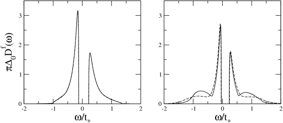
Figure 14: Weak coupling LMA $f$-electron spectrum (solid line) vs ${\omega}/t_{*}$ for the Bethe lattice, with $U=0.75$ (right panel) and $U=0.25$ (left panel); and for ${\epsilon}_{c}=0.2$, $\eta=0$ and $V^{2}=0$. Corresponding results from second order perturbation theory in $U$ are also shown (dashed lines); for the lower-$U$ shown this is indistinguishable from the LMA spectrum.

The obvious conclusion from the preceding discussion is that we find no compelling evidence for two-scale exhaustion. A sceptic can naturally argue that since the present theory is approximate it is open to doubt. That is of course true, as it is for any theory. But the evidence here certainly points away from exhaustion and, should further support for the idea be forthcoming, it will in our view require convincing scaling arguments to be established.

6 Concluding remarks

We have developed in this paper a local moment approach to single-particle dynamics of the periodic Anderson model within the framework of dynamical mean-field theory, for the generic asymmetric case relevant to heavy fermion metals. For obvious physical reasons our primary interest has been the strongly correlated Kondo lattice regime, of essentially localized spins $n_{f}\rightarrow 1$ but with general conduction band filling $n_{c}$, which the intrinsically non-perturbative nature of the LMA renders readily accessible. The exponentially small lattice coherence scale ${\omega}_{L}$ inherent to the Kondo lattice regime leads in particular to a clean separation of low-energy (‘universal’) and high-energy scales, and hence to universal scaling behaviour of dynamics. This has been a central focus of the present work and a rich description of scaling spectra results, spanning all ${\omega}/{\omega}_{L}$-scales. With increasing ${\omega}^{\prime}={\omega}/{\omega}_{L}$, dynamics are found to cross over from the low-energy quasiparticle behaviour symptomatic of the coherent Fermi liquid state to essentially incoherent single-impurity Anderson/Kondo scaling physics at high-${\omega}^{\prime}$. The former, low-${\omega}^{\prime}$ behaviour depends naturally on both the conduction band filling and underlying lattice ‘type’. The latter by contrast depends on neither, consistent with one’s physical expectation of effective single-impurity physics; and the crossover from coherent Fermi liquid to effective single-impurity behaviour in the PAM, established as it is by scaling, neither presumes nor requires any particular relation between the PAM coherence scale, ${\omega}_{L}$, and the Kondo scale ${\omega}_{K}$ for the corresponding ‘real’ AIM arising when only a single $f$-level is coupled to the conduction band.

While our almost exclusive emphasis has been on the strongly correlated regime we add that, as for the Anderson impurity models considered hitherto [26,27], all interaction strengths are nonetheless encompassed by the LMA including simple perturbative behaviour in weak coupling – an illustration of the latter being given in Fig.14 where, for $U=0.75$ and $0.25$ (with ${\epsilon}_{c}=0.2,\eta=0$ and $V^{2}=0.2$) LMA results for the $f$-electron spectrum $\pi\Delta_{0}D^{f}({\omega})$ vs ${\omega}/t_{*}$ are compared to those arising from second order perturbation theory (PT) in the interaction $U$: with decreasing interaction the LMA spectrum clearly reduces to that arising from PT, being indistinguishable from it for the lower $U$ shown.

The essential criteria for a successful description of the PAM thus appear to be met by the LMA; all energy scales, and interaction strengths from weak to strong coupling, being handled in a unified theoretical framework. Further (as mentioned in §1), a description of the single-particle dynamics considered here is a prerequisite to determining transport and optical properties of heavy fermions; which subject, including explicit comparison to experiment, will be considered in a forthcoming paper.

- (1) N. Grewe, F. Steglich, Handbook on the Physics and Chemistry of Rare Earths, edited by K. A. Gschneider Jr. and L. L. Eyring (Elsevier, Amsterdam, 1991), Vol. 14, 343
- (2) A. C. Hewson, The Kondo Problem to Heavy Fermions (Cambridge University Press, Cambridge, 1993)
- (3) D. Vollhardt, Correlated Electron Systems Vol. 9, edited by V. J. Emery (World Scientific, Singapore, 1993)
- (4) T. Pruschke, M. Jarrell, J. K. Freericks, Adv. Phys. 44, 187 (1995)
- (5) A. Georges, G. Kotliar, W. Krauth, M. Rozenberg, Rev. Mod. Phys. 68, 13 (1996)
- (6) F. Gebhard, The Mott Metal-Insulator Transition (Springer Tracts in Modern Physics, Vol. 137) (Springer, Berlin, 1997)
- (7) Y. Shimizu, O. Sakai, Computational Physics as a New Frontier in Condensed Matter Research, edited by H. Takayama et al. (The Physical Society of Japan, Tokyo, 1995), p.42
- (8) T. Pruschke, R. Bulla, M. Jarrell, Phys. Rev. B 61, 12799 (2000)
- (9) M. Jarrell, H. Akhlaghpour, T. Pruschke, Phys. Rev. Lett. 70, 1670 (1993)
- (10) M. Jarrell, Phys. Rev. B 51, 7429 (1995)
- (11) A. N. Tahvildar-Zadeh, M. Jarrell, J. K. Freericks, Phys. Rev. B 55, R3332(1997); Phys. Rev. Lett. 80, 5168 (1998)
- (12) A. N. Tahvildar-Zadeh, M. Jarrell, T. Pruschke, J. K. Freericks, Phys. Rev. B 60, 10782 (1999)
- (13) M. J. Rozenberg, Phys. Rev. B 52, 7369 (1995)
- (14) H. Schweitzer, G. Czycholl, Solid State Commun. 69, 179 (1989)
- (15) H. Schweitzer, G. Czycholl, Phys. Rev. Lett. 67, 3724 (1991)
- (16) M. J. Rozenberg, G. Kotliar, H. Kajueter, Phys. Rev. B 54, 8452 (1996)
- (17) N. S. Vidhyadhiraja, A. N. Tahvildar-Zadeh, M. Jarrell, H. R. Krishnamurthy, Europhys. Lett. 49, 459 (2000)
- (18) N. Grewe, T. Pruschke, H. Keiter, Z. Phys. B: Condens. Matt. 71, 75 (1988)
- (19) T. Pruschke, N. Grewe, Z. Phys B: Condens. Matt. 74, 439 (1989)
- (20) D. L. Cox, N, Grewe, Z. Phys B: Condens. Matt. 71, 321 (1988)
- (21) D. M. Newns, N. Read, Adv. Phys. 36, 799 (1987)
- (22) S. J. Sun, M. F. Yang, T. M. Hong, Phys. Rev. B 48, 16127 (1993)
- (23) S. Burdin, A. Georges, D. R. Grempel, Phys. Rev. Lett. 85, 1048 (2000)
- (24) T. M. Rice, K. Ueda, Phys. Rev. B 34, 6420 (1986)
- (25) P. Fazekas, B. H. Brandow, Physica Scripta 36(5), 809 (1987); P. Fazekas, J. Magn. Magn. Mat. 63 & 64, 545 (1987)
- (26) D. E. Logan, M. P. Eastwood, M. A. Tusch, J. Phys. Condens. Matt. 10, 2673 (1998)
- (27) M. T. Glossop, D. E. Logan, J. Phys. Condens. Matt. 14, 6737 (2002)
- (28) N. L. Dickens, D. E. Logan, J. Phys. Condens. Matt. 13, 4505 (2001)
- (29) D. E. Logan, N. L. Dickens, J. Phys. Condens. Matt. 14, 3605 (2002)
- (30) D. E. Logan, N. L. Dickens, Europhys. Lett. 54, 227 (2001); D. E. Logan, N. L. Dickens, J. Phys. Condens. Matt. 13, 9713 (2001)
- (31) D. E. Logan, M. T. Glossop, J. Phys. Condens. Matt. 12, 985 (2000)
- (32) M. T. Glossop, D. E. Logan, J. Phys. Condens. Matt. 15, 7519 (2003); M. T. Glossop, D. E. Logan, Europhys. Lett. 61, 810 (2003)
- (33) R. Bulla, M. T. Glossop, D. E. Logan, T. Pruschke, J. Phys. Condens. Matt. 12, 4899 (2000)
- (34) V. E. Smith, D. E. Logan, H. R. Krishnamurthy, Eur. Phys. J. B 32, 49 (2003)
- (35) N. S. Vidhyadhiraja, V. E. Smith, D. E. Logan, H. R. Krishnamurthy, J. Phys. Condens. Matt. 15, 4045 (2003)
- (36) J. M. Luttinger, J. C. Ward, Phys. Rev. 118, 1417 (1960)
- (37) P. Nozires, Ann. Phys. (Paris) 10, 19 (1985)
- (38) P. Nozires, Eur. Phys. J. B 6, 447 (1998)
- (39) E. Feenberg, Phys. Rev. 74, 206 (1948)
- (40) E. N. Economou, Green’s Functions in Quantum Mechanics, (Springer, Berlin, 1983)
- (41) P. Wachter, Handbook on the Physics and Chemistry of Rare Earths, edited by K. A. Gschneider and L.L. Eyring (Elsevier, Amsterdam, 1994), Vol. 19, p. 177
- (42) D. C. Langreth, Phys. Rev. 150, 516 (1966)
- (43) D. M. Edwards, Narrow Band Phenomena, NATO ASI Series (Plenum, New York, 1988)
- (44) M. Jarrell, Phys. Rev. Lett. 69, 168 (1992)
- (45) W. Shakespeare, Romeo and Juliet, edited by W. J. Craig (Oxford University Press, Oxford, 1914)
- (46) D. E. Logan, M. P. Eastwood and M. A. Tusch, J. Phys. Condens. Matt. 9, 4211 (1997)