Ordering of droplets and light scattering in polymer dispersed liquid crystal films

Abstract

We study the effects of droplet ordering in initial optical transmittance through polymer dispersed liquid crystal (PDLC) films prepared in the presence of an electrical field. The experimental data are interpreted by using a theoretical approach to light scattering in PDLC films that explicitly relates optical transmittance and the order parameters characterizing both the orientational structures inside bipolar droplets and orientational distribution of the droplets. The theory relies on the Rayleigh-Gans approximation and uses the Percus-Yevick approximation to take into account the effects due to droplet positional correlations.

I Introduction

Polymer dispersed liquid crystal (PDLC) films consist of randomly distributed micrometer-sized liquid crystal (LC) droplets embedded in an isotropic polymer matrix, and have attracted considerable interest for both technological and for more fundamental reasons Doane (1990); Drzaic (1995); Crawford and Žumer (1996); Higgins (2000).

The droplets are typically filled with a nematic liquid crystal (NLC). Optical characteristics of such birefringent nematic droplets differ from those of the surrounding polymer matrix and the droplets can be viewed as optically anisotropic inhomogeneities which scatter light incident upon them.

Optical transmittance of PDLC films is mostly determined by light scattering properties of NLC droplets that crucially depend on NLC orientational structure. This structure can be influenced by an external electrical field which reorients the NLC directors inside the droplets and thereby light scattering in the film appears to be governed by the field. This mechanism underlies the mode of operation of PDLC films that, under certain conditions, can be switched from an opaque to a clear state by applying an electric voltage.

Schematic representation of the field effect on the orientational structure is given in Fig. 1. The zero-field case in which orientation of NLC is randomly distributed over the droplets is shown in Fig. 1(a). As is illustrated in Fig. 1(b), in the presence of a field, the NLC directors align along the prescribed direction $\mathbf{\hat{N}}$. When the polymer index of refraction, $n_{p}$, and the ordinary refractive index of NLC, $n_{lc}^{(o)}$, are matched, the PDLC film in the on state is almost transparent for waves propagating along the voltage induced anisotropy axis $\mathbf{\hat{N}}$.

Optical switching contrast, which is the ratio of the transmittance in the on state and the initial (zero-field) transmittance, is an important characteristic of the PDLC film. High switching contrast can be achieved by reducing the zero-field transmittance of the PDLC film and, for this purpose, the film should be prepared so as to maximize optical contrast between the polymer and NLC.

Typically, the extraordinary refractive index $n_{lc}^{(e)}$ is the largest value of the NLC refractive index and $n_{lc}^{(o)}\approx n_{p}<n_{lc}^{(e)}$. So, for light normally incident upon the film, in-plane alignment of NLC inside the droplets will enhance scattering efficiency. The experimental procedures for stimulating NLC molecules to be aligned in the plane of the PDLC film were suggested in Refs. Doane (1990); Margerum et al. (1985); Wu and Wang (1997). In these methods the film of PDLC precursor was subjected to external fields [mechanical pressure, light, electrical and magnetic fields] during the phase separation.

In this paper we present both experimental and theoretical results for initial transmittance of PDLC films prepared in the presence of an electrical field applied across the film of PDLC precursor. In this case the voltage will align NLC molecules perpendicular to the film thus reducing the switching contrast. We are, however, primarily interested in studying relation between the optical transmittance of a PDLC film and the order parameters characterizing both the orientational structures inside the droplets and overall anisotropy of the film.

To this end, we need to have a theory that explicitly relates the order parameters and the transmittance to interpret the experimental data. In Refs. Bloisi et al. (1995, 1996) the theory by Kelly and Palffy-Muhoray Kelly and Palffy-Muhoray (1994), that studied the electrical field induced effects in light scattering by an ensemble of bipolar droplets, has been used to discuss the order parameter effects in optical transmittance through a PDLC film.

In the present paper these effects will be studied by using a more comprehensive approach that takes into account interference effects caused by droplet positional correlations. As in Ref. Cox et al. (1998), for this purpose, we shall use the Percus-Yevick approximation. We also combine the effective medium theory Levy (2000) with the low concentration approximation to account for the dependent scattering effects.

The paper is organized as follows. In Sec. II, we give necessary details on the experimental procedure used in this study and describe the morphology of the PDLC system under consideration. We present the experimentally measured dependencies of the zero-field transmittance and the transmittance in the saturated on state on the voltage $U_{uv}$ applied across the film during UV polymerization.

Our theoretical considerations are presented in Sec. III. We characterize NLC director structures inside the bipolar droplets and the orientational distribution of the bipolar axis by the bipolar order parameter $Q_{\mathrm{d}}$ and the order parameter $Q$. Then we compute the effective dielectric constant and use the Rayleigh-Gans approximation to evaluate the scattering cross section of a bipolar droplet embedded in the effective medium. After averaging the cross section over both positions and orientation of bipolar droplets we derive the scattering mean free path and the optical transmittance. Dependencies of the transmittance on the order parameters at different droplet sizes are calculated numerically.

In Sec. IV, we draw together and discuss our results. The experimental data are interpreted by using the theoretical results. The order parameters in the off state are estimated. The value of the bipolar order parameter $Q_{\mathrm{d}}$ is found to be about $0.85$. For samples prepared with no applied voltage, the order parameter $Q$ turns out to be very close to zero. This order parameter rapidly grows and saturates as the voltage $U_{uv}$ increases. Finally, we conclude in Sec. V.

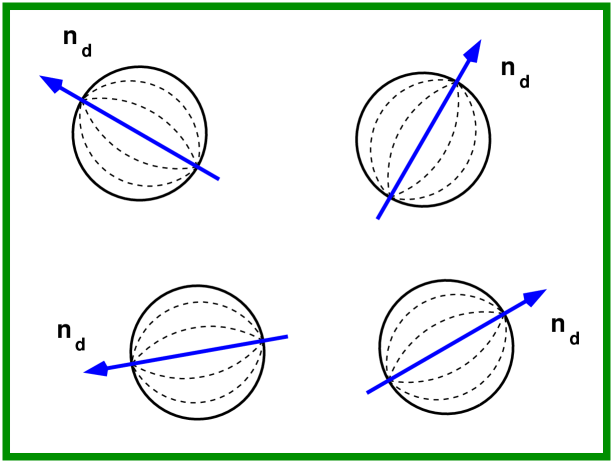
(a) Off state with $Q=0$

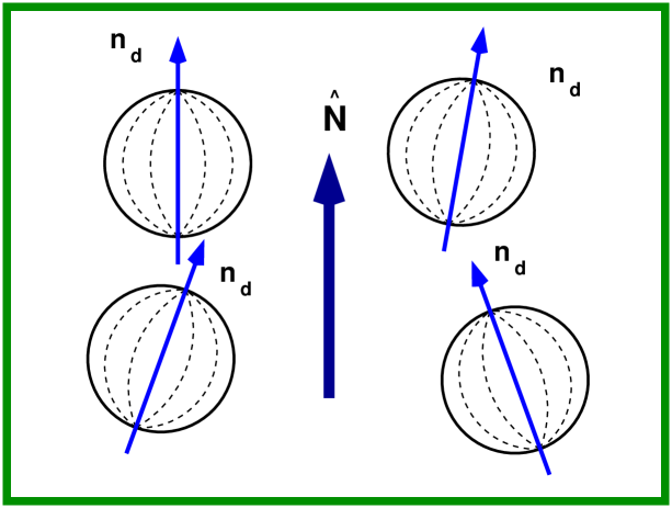
(b) On state with $Q\approx 1$

Figure 1: (a) Random and (b) uniaxially anisotropic orientational distributions of bipolar droplets.

Figure 2: $T$-$U$ dependences for two PDLC samples prepared at (a) $U_{uv}=0$ V and (b) $U_{uv}=20$ V. Arrows indicate an increase and a decrease of the applied voltage $U$.

Figure 3: SEM image of PDLC layer ($c_{p}=60$ wt%, $c_{lc}=40$ wt%).

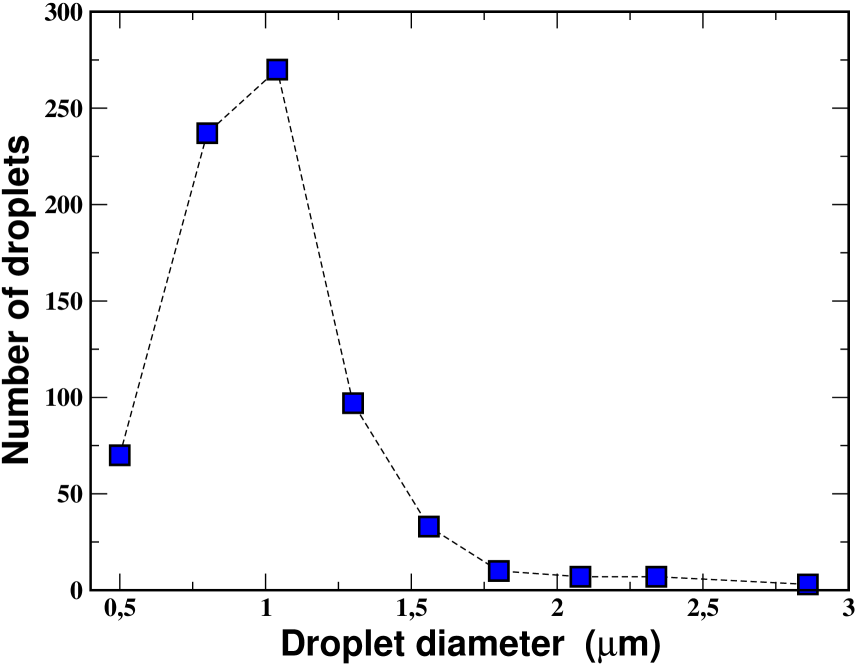
Figure 4: Distribution of droplet sizes in PDLC layer ($c_{p}=60$ wt%, $c_{lc}=40$ wt%).

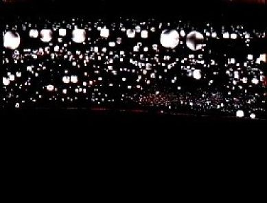
(a) $U_{uv}=0$ V

(b) $U_{uv}=40$ V

Figure 5: Periphery part of PDLC layers as viewed in polarizing microscope. The layers are preparated at (a) $U_{uv}=0$ V and (b) $U_{uv}=40$ V. It is clearly seen that the bipolar droplets are orientationally disordered at $U_{uv}=0$ V and are oriented along the field at $U_{uv}=40$ V.

II Experimental

II.1 Sample preparation

NLC mixture E7 from Merck and UV curable adhesive POA65 from Norland Inc.(USA) were used to prepare the composite. PDLC systems based on these components have been studied intensively  Wu and Wang (1997); Bhargava et al. (1999a, b, c); Dolgov and Yaroshchuk (2003).

The components were thoroughly mixed. The content of LC and polymer precursor in the mixture was $c_{p}=60$ wt% and $c_{lc}=40$ wt%, respectively. The mixing was performed under red light so as to avoid early polymerization of POA65. The prepared mixture was sandwiched between two glass slabs covered with ITO on the inner side. The cell gap was maintained by spacer balls 20 $\mu$m in size. The substrates were pressed and glued with a epoxy glue.

In order to stimulate polymerization-induced phase separation leading to the formation of PDLC layers the samples were irradiated with the light from mercury lamp. The intensity and the time of irradiation were 100 mW/cm² and 20 min, respectively.

The samples were subjected to the electrical field $U_{uv}$ of the frequency $f=2$ kHz during UV polymerization. The voltages $U_{uv}=$0 V, 2 V, 10 V, 20 V, 50 V and 100 V were applied across the samples to prepare PDLC layers with varying orientational distribution of droplets and, as a result, initial transmittance. The difference in transmittance was visible even to the human eye.

SEM measurements were carried out using device S-2600N from Hitachi. For performing the measurements the samples were treated as follows. One glass slab was removed and the remaining part of the sample was immersed into ethanol of purity 98% for 24 h. Then the sample was taken out from ethanol, dried and coated with gold.

II.2 Optical transmittance

Optical transmittance $T$ versus applied voltage $U$ curves were measured at room temperature using the computer conjugated measuring system previously described in Ref. Zakrevska et al. (2002). The sample transmittance was defined as the ratio:

$$T=\frac{I_{out}}{I_{in}},$$ (1)

where $I_{in}$ is the intensity of the normally incident light with the wavelength $\lambda=635$ nm and $I_{out}$ is the intensity of the light transmitted through the sample. Following usual procedure, the non-scattered light and the light scattered within the angle of 2 degrees were detected with a photodiode. The $T$-$U$ curves were measured at both increasing and decreasing voltage. In this process, the voltage was varied from 0 V to 100 V, whereas the frequency was fixed at 2 kHz. Typical $T$-$U$ curves are shown in Fig. 2. As is indicated, the curves provide transmittance in the initial zero-field state ($T_{0}$) and in a state of saturation reached at sufficiently large voltages ($T_{sat}$).

Experiment			Theory
$U_{uv}$ (V)	$T_{0}$ (%)	$T_{sat}$ (%)	$Q_{\mathrm{d}}=0.85$		$Q_{\mathrm{d}}=0.9$
expt.	expt.	expt.	$T_{0}$ (%)	$Q$	$T_{0}$ (%)	$Q$
$0$	$8$	$97$	$9.0$	$0.04$	$7.0$	$0.05$
$2$	$10$	$97$	$10.04$	$0.25$	$10.3$	$0.4$
$10$	$13$	$90$	$12.9$	$0.4$	$13.0$	$0.49$
$20$	$40$	$95$	$39.8$	$0.775$	$40.5$	$0.8$
$50$	$84$	$99$	$83.5$	$0.96$	$83.6$	$0.97$
$100$	$88$	$99$	$87.5$	$0.97$	$89.0$	$0.98$

Table 1: Zero-field and saturated transmittance, $T_{0}$ and $T_{sat}$, measured at different values of the voltage $U_{uv}$ applied during polymerization (the film thickness is $20\,\mu$m and the accuracy of the measurements is about $\pm 0.7$%). The corresponding theoretical values of $T_{0}$ and the order parameter $Q$ are given in the last four columns.

II.3 Experimental results

A typical SEM image and the corresponding distribution of droplet sizes are shown in Fig. 3 and in Fig. 4, respectively. It is seen that the preparation procedure yields the well-known “Swiss cheese” PDLC morphology with a uniform spatial distribution of the droplets. We did not observe an anisotropy of droplet shape in the probes prepared in the presence of the field. The droplet size distribution is rather narrow. The prevailed droplet diameter is about 1 $\mu$m.

The director configuration inside NLC droplets with diameters of about 5 $\mu$m can be identified by observation in polarizing microscope. Such large droplets often form in outlying parts of PDLC layers during phase separation. The pictures typical of PDLC formed at $U_{uv}=0$ V and $U_{uv}=40$ V are shown in Fig. 5(a) and in Fig. 5(b), respectively. It is seen that the droplets are spherically shaped regardless of the field applied during phase separation. The bipolar structure inside the droplets can also be clearly observed. For the sample prepared at $U_{uv}=0$, the droplets are randomly oriented, whereas the droplets in the sample obtained at $U_{uv}=40$ V are aligned along the direction of the applied field.

For the concentrations of the components used in our samples (60 wt% of polymer and 40 wt% of NLC), the concentration of NLC droplets is not large. It is confirmed by weak scattering of light in these composites.

For PDLC based on our components, the fractions of NLC confined in droplets and of NLC dissolved in the polymer matrix were obtained from IR measurements in Ref. Bhargava et al. (1999b). According to these results, in our case only about 30 % of NLC phase separates. Assuming that the density of polymer is 1.5 g/cm³ and the density of E7 is 1.05 g/cm³, we can estimate the volume fraction of droplets, $\eta$, to be about 23.5 vol%.

The obtained data are summarized in Table 1, where the values of the transmittance in the off state $T_{0}$ and the transmittance in the saturated state $T_{sat}$ measured for different values of the voltage $U_{uv}$ applied during phase separation. It can be concluded that the transmittance in the saturated state $T_{sat}$ is almost insensitive to the voltage $U_{uv}$ applied during phase separation as opposed to the initial transmittance $T_{0}$ which rapidly grows with $U_{uv}$ and eventually saturates.

III Theory

III.1 Model and order parameters

In this section our task is to study the problem of light scattering by an ensemble of partially ordered spherical NLC droplets dispersed in an optically isotropic polymer matrix with the dielectric constant $\epsilon_{p}$ and the refractive index $n_{p}=\sqrt{\epsilon_{p}}$. The ensemble of such droplets can be regarded as a reasonably simplified model of a PDLC system.

Specifically, we consider the case in which NLC is tangentially ordered at the droplet surfaces and the NLC director field $\mathbf{\hat{n}}_{\mathrm{LC}}$ inside the droplet forms the bipolar orientational structure. The symmetry of this structure is cylindrical and there are boojum surface singularities at the droplet poles defined by the symmetry (bipolar) axis of the bipolar configuration $\mathbf{\hat{n}}_{\mathrm{d}}$.

The bipolar droplets are optically anisotropic with the dielectric tensor

$$\boldsymbol{\epsilon}_{\mathrm{LC}}=\epsilon_{\perp}^{(lc)}\,\mathbf{I}+\epsilon_{a}^{(lc)}\,\mathbf{\hat{n}}_{\mathrm{LC}}\otimes\mathbf{\hat{n}}_{\mathrm{LC}},$$ (2)

where $\epsilon_{a}^{(lc)}=\epsilon_{\parallel}^{(lc)}-\epsilon_{\perp}^{(lc)}$ and $\mathbf{I}$ is the identity matrix. Thus, the refractive indices of ordinary and extraordinary waves are: $n_{o}^{(lc)}=\sqrt{\epsilon_{\perp}^{(lc)}}$ and $n_{e}^{(lc)}=\sqrt{\epsilon_{\parallel}^{(lc)}}$, respectively.

We shall also need to introduce the dielectric tensor averaged over the director distribution inside a droplet $\left\langle{\boldsymbol{\epsilon}_{\mathrm{LC}}}\right\rangle_{lc}\equiv\boldsymbol{\epsilon}_{\mathrm{d}}$. Owing to the cylindrical symmetry of the orientational structure, each bipolar droplet can be characterized by the nematic-like tensorial order parameter

$$\left\langle{(3\mathbf{\hat{n}}_{\mathrm{LC}}\otimes\mathbf{\hat{n}}_{\mathrm{LC}}-\mathbf{I})/2}\right\rangle_{lc}=Q_{\mathrm{d}}(3\mathbf{\hat{n}}_{\mathrm{d}}\otimes\mathbf{\hat{n}}_{\mathrm{d}}-\mathbf{I})/2,$$ (3)

so that the average dielectric tensor of a bipolar droplet $\boldsymbol{\epsilon}_{\mathrm{d}}$ is

$$\boldsymbol{\epsilon}_{\mathrm{d}}=\left\langle{\boldsymbol{\epsilon}_{\mathrm{LC}}}\right\rangle_{lc}=\epsilon_{\perp}\,\mathbf{I}+\epsilon_{a}\,\mathbf{\hat{n}}_{\mathrm{d}}\otimes\mathbf{\hat{n}}_{\mathrm{d}},$$ (4)

where $\epsilon_{\perp}=\epsilon_{\perp}^{(lc)}+\epsilon_{a}^{(lc)}(1-Q_{\mathrm{d}})/3$ and $\epsilon_{a}\equiv\epsilon_{\parallel}-\epsilon_{\perp}=\epsilon_{a}^{(lc)}Q_{\mathrm{d}}$.

By analogy to the bipolar axis $\mathbf{\hat{n}}_{d}$ which defines the droplet orientation, the scalar order parameter $Q_{\mathrm{d}}$ will be referred to as the bipolar order parameter. This parameter characterizes the degree of droplet anisotropy that depends on distortions of the director field with respect to the uniform configuration aligned along the bipolar axis.

In general, the value of $Q_{\mathrm{d}}$ varies depending on a number of factors such as droplet size and shape, anchoring conditions, applied voltage and so on. In Ref. Cox et al. (1998), such variations are found to be negligible and the bipolar order parameter was estimated to be about $0.82$. By contrast, the results of Refs. Bloisi et al. (1995, 1996) suggest that the bipolar order parameter of a PDLC film can be considerably affected by an applied electric voltage.

In any event, so long as size and shape polydispersity is weak, variations of the bipolar order parameter throughout a sample can be reasonably disregarded. From the other hand, it is now commonly accepted that disorder in positions and orientation of bipolar droplets is of vital importance for an understanding of light scattering in PDLC systems Žumer et al. (1989); Kelly and Palffy-Muhoray (1994); Cox et al. (1998). When the orientational distribution of the bipolar axis is uniaxial, the relation of the form similar to Eq. (3)

$$\left\langle{(3\mathbf{\hat{n}}_{\mathrm{d}}\otimes\mathbf{\hat{n}}_{\mathrm{d}}-\mathbf{I})/2}\right\rangle_{d}=Q(3\mathbf{\hat{N}}\otimes\mathbf{\hat{N}}-\mathbf{I})/2$$ (5)

describes this distribution in terms of the order parameter $Q$ and the optical axis $\mathbf{\hat{N}}$.

When direction of the bipolar axis is randomly distributed, the PDLC film is isotropic and $Q=0$. This case is illustrated in Fig. 1(a). The initial off state of a PDLC film is often assumed to be isotropic.

Applying an external electric field will reorient NLC inside the droplets so as to introduce an overall anisotropy of the sample with the optical axis $\mathbf{\hat{N}}$ parallel to the field. Fig. 1(b) schematically shows a distribution of this sort. The limiting case where all the droplets are aligned along the field direction corresponds to the on state of a PDLC film in the regime of saturation (the saturated state) with $Q=1$.

The effect of the order parameters $Q_{\mathrm{d}}$ and $Q$ on light scattering in PDLC films will be of our major concern.

III.2 Effective dielectric tensor

The films under consideration exemplify an inhomogeneous medium in which a host material and isolated inclusions are clearly identified. Our first step is to determine effective dielectric characteristics of the film in the long wavelength limit. To this end, we restrict ourselves to the case where the droplets are well separated and the volume fraction of droplets, $\eta$, is not too high.

Under these conditions, following Refs. Cox et al. (1996); Levy (2000), we may use the excluded volume approximation discussed by Landauer in Ref. Landauer (1978) and write the total average electric field $\mathbf{E}$ as

$$\mathbf{E}=\eta\mathbf{E}_{\mathrm{d}}+(1-\eta)\mathbf{E}_{p},$$ (6)

where $\mathbf{E}_{p}$ and $\mathbf{E}_{\mathrm{d}}$ are the average electric fields in the polymer matrix and inside the droplets, respectively. Using the relation for the mean electric polarization vectors: $\mathbf{P}$, $\mathbf{P}_{\mathrm{d}}$ and $\mathbf{P}_{p}$, that can be written by analogy with Eq. (6), we have

$$\boldsymbol{\epsilon}_{\mathrm{eff}}\mathbf{E}=\eta\boldsymbol{\epsilon}_{\mathrm{d}}\mathbf{E}_{\mathrm{d}}+(1-\eta)\epsilon_{p}\mathbf{E}_{p}.$$ (7)

In Eq. (7) the orientationally averaged dielectric tensor (4) is used as an approximation for the dielectric tensor averaged over the droplets.

The fields $\mathbf{E}_{\mathrm{d}}$ and $\mathbf{E}_{p}$ can now be related by means of an anisotropic version of the traditional Maxwell-Garnett closure Cox et al. (1996); Levy (2000) (reviews of other approximate schemes can be found in van Beek (1967); Landauer (1978); Bergman and Stroud (1992)):

$$\mathbf{E}_{p}=\mathbf{M}\mathbf{E}_{\mathrm{d}},\quad\mathbf{M}=(2\epsilon_{p}\,\mathbf{I}+\boldsymbol{\epsilon}_{\mathrm{d}})/(3\epsilon_{p}).$$ (8)

Combining Eqs. (6), (7) and (8) gives the final result for $\boldsymbol{\epsilon}_{\mathrm{eff}}$:

$$\boldsymbol{\epsilon}_{\mathrm{eff}}=\epsilon_{p}\mathbf{I}+\eta\,\left\langle{(\boldsymbol{\epsilon}_{\mathrm{d}}-\epsilon_{p}\mathbf{I})\mathbf{M}^{-1}}\right\rangle$$

$$\times\bigl{[}\eta\,\left\langle{\mathbf{M}^{-1}}\right\rangle+(1-\eta)\mathbf{I}\bigr{]}^{-1}=\epsilon_{m}\mathbf{I}+\Delta\epsilon_{m}\mathbf{\hat{N}}\otimes\mathbf{\hat{N}},$$ (9)

$$\epsilon_{m}=\epsilon_{p}\frac{\epsilon_{\perp}+2\epsilon_{p}+2\eta\epsilon_{1}}{\epsilon_{\perp}+2\epsilon_{p}-\eta\epsilon_{1}}\approx\epsilon_{p}+\eta\epsilon_{1},$$ (10)

$$\Delta\epsilon_{m}=9\epsilon_{p}^{2}\epsilon_{a}\eta\,\frac{\epsilon_{\perp}+2\epsilon_{p}}{\epsilon_{\parallel}+2\epsilon_{p}}\,\Bigl{[}(\epsilon_{\perp}+2\epsilon_{p}-\eta\epsilon_{1})(\epsilon_{\perp}+2\epsilon_{p}-\eta\epsilon_{2})\Bigr{]}^{-1},$$ (11)

where $\epsilon_{1}=\epsilon_{\perp}-\epsilon_{p}+\epsilon_{p}\epsilon_{a}(1-Q)/(\epsilon_{\parallel}+2\epsilon_{p})$ and $\epsilon_{2}=\epsilon_{\perp}-\epsilon_{p}+\epsilon_{p}\epsilon_{a}(1+2Q)/(\epsilon_{\parallel}+2\epsilon_{p})$.

For the polymer with $n_{p}=1.54$ and the liquid crystal mixture E7 with $n_{o}^{(lc)}=1.5216$ and $n_{e}^{(lc)}=1.74$, it can be verified that the linear relation on the right hand side of Eq. (10) gives a good approximation for the volume fraction dependence of the effective dielectric constant $\epsilon_{m}$. This is a modified version of the mixing rule $\epsilon_{m}=(1-\eta)\epsilon_{p}+\eta\epsilon_{\perp}$ used in Ref. Cox et al. (1998).

Eq. (11) clearly indicates that, in general, the anisotropic part of the effective dielectric tensor does not vanish. But the effective anisotropy parameter $\Delta\epsilon_{m}/\epsilon_{m}$ is found to be well under $0.05$, so that the effective medium is weakly anisotropic as compared to NLC inside the droplets, where $\epsilon_{a}^{(lc)}/\epsilon_{\perp}^{(lc)}>0.3$. For this reason, as in Refs. Kelly and Palffy-Muhoray (1994); Basile et al. (1993); Bloisi et al. (1995, 1996); Cox et al. (1998), anisotropy of the effective medium can be disregarded.

In our subsequent treatment of the light scattering problem we shall use the relation (10) to account for the dependent scattering effects by replacing the polymer matrix surrounding the droplets with the effective medium. It is, however, should be noted that the result (10) is strictly valid only in the Rayleigh limit where the scatterer size is much smaller than the wavelength of light (an extended discussion can be found in Chap. 9 of Ref. Mishchenko et al. (2000)). This result can also be derived from the self-consistency condition that requires vanishing the average scattering amplitude in the forward direction for droplets embedded in the effective medium Stroud and Pan (1978). So, the effective dielectric constant (10) serves as the lowest order approximation of a coherent potential approach Soukoulis et al. (1994).

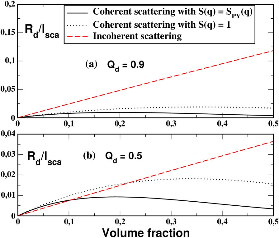
Figure 6: Coherent and incoherent light scattering contributions to the ratio $R_{\mathrm{d}}/l_{sca}$ versus the volume fraction $\eta$ at $R_{\mathrm{d}}=0.5\mu$m for two values of the bipolar order parameter $Q_{\mathrm{d}}$: (a) $Q_{\mathrm{d}}=0.9$ and (b) $Q_{\mathrm{d}}=0.5$. Refractive indices used in calculations are: $n_{p}=1.54$, $n_{o}^{(lc)}=1.52$ and $n_{e}^{(lc)}=1.74$.

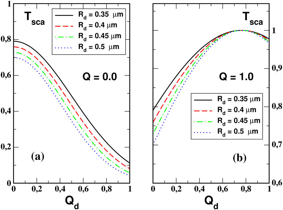
Figure 7: Transmittance as a function of the bipolar order parameter $Q_{\mathrm{d}}$ at the volume fraction $\eta=0.235$ for different droplet radii and two values of the order parameter $Q$: (a) $Q=0$ and (b) $Q=1$.

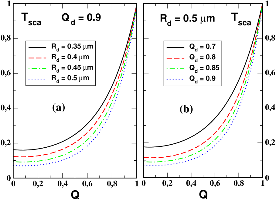
Figure 8: Transmittance as a function of the order parameter $Q$ at (a) various values of the mean droplet radius $R_{\mathrm{d}}$ for $Q_{\mathrm{d}}=0.9$ and at (b) various values of the bipolar order parameter $Q_{\mathrm{d}}$ for $R_{\mathrm{d}}=0.5\mu$m. The droplet volume fraction is $0.235$ and the thickness of PDLC layer is $20\,\mu$m.

III.3 Light scattering and optical transmittance

In this section we begin with the light scattering problem for a single LC droplet characterized by the average dielectric tensor (4) and surrounded by the medium with the effective refractive index $n_{m}=\sqrt{\epsilon_{m}}$. Using the well-known Rayleigh-Gans approximation Ishimaru (1978); Newton (1982), we compute the elements of the scattering amplitude matrix and the scattering cross section.

Then we apply the Percus-Yevick approximation Percus and Yevick (1958); Ziman (1979) to evaluate the effective scattering as the scattering cross section averaged over positions of the droplets and perform averaging of the scattering cross section over the bipolar axis orientation. Finally, in the low concentration approximation, we derive the expressions for the scattering mean free path and the optical transmittance.

III.3.1 Scattering amplitude matrix in Rayleigh-Gans approximation

Following the standard procedure Ishimaru (1978); Newton (1982), the undisturbed incident wave is assumed to be a harmonic plane wave with the frequency $\omega$ and the wavenumber $k=n_{m}\omega/c$. The wave is propagating through the effective medium along the direction specified by a unit vector $\mathbf{\hat{k}}_{inc}$ and the wave vector $\mathbf{k}_{inc}=k\mathbf{\hat{k}}_{inc}$. The polarization vector of the electric field is

$$\mathbf{E}_{inc}={E}_{i}^{(inc)}\,\mathbf{\hat{e}}_{i}(\mathbf{\hat{k}}_{inc}),$$ (12)

where the basis vectors $\mathbf{\hat{e}}_{x}(\mathbf{\hat{k}}_{inc})=(\cos\theta_{i}\cos\phi_{i},\cos\theta_{i}\sin\phi_{i},-\sin\theta_{i})$ and $\mathbf{\hat{e}}_{y}(\mathbf{\hat{k}}_{inc})=(-\sin\phi_{i},\cos\phi_{i},0)$ are perpendicular to $\mathbf{\hat{k}}_{inc}$ defined by the polar and azimuthal angles: $\theta_{i}$ and $\phi_{i}$. [Throughout the paper summation over repeated indices will be assumed.]

Asymptotic behavior of the scattered outgoing wave in the far field region ($kr\gg 1$) is known Ishimaru (1978); Newton (1982):

$$\mathbf{E}_{sca}(\mathbf{r})\sim\mathbf{E}_{sca}\frac{\mathrm{e}^{ikr}}{kr},\quad\mathbf{E}_{sca}={E}_{i}^{(sca)}\,\mathbf{\hat{e}}_{i}(\mathbf{\hat{k}}_{sca}),$$ (13)

where $\mathbf{\hat{k}}_{sca}=\mathbf{\hat{r}}=(\sin\theta\cos\phi,\sin\theta\sin\phi,\cos\theta)$ and $\mathbf{E}_{sca}$ is linearly related to the polarization vector of the incident wave (12) through the scattering amplitude matrix $\mathbf{A}(\mathbf{k}_{sca},\mathbf{k}_{inc})$ in the following way:

$${E}_{i}^{(sca)}=A_{ij}(\mathbf{k}_{sca},\mathbf{k}_{inc}){E}_{j}^{(inc)}.$$ (14)

The elements of the scattering amplitude matrix can be easily computed by using the Rayleigh-Gans approximation (RGA) Ishimaru (1978); Newton (1982). This approximation is known to be applicable to the case of submicron nematic droplets Žumer and Doane (1986); Cox et al. (1998); Leclercq et al. (1999) and gives the following result:

$$A_{ij}(\mathbf{\hat{k}}_{sca},\mathbf{\hat{k}}_{inc})=\frac{V_{\mathrm{d}}k^{3}}{4\pi}\,\mathbf{\hat{e}}_{i}(\mathbf{\hat{k}}_{sca})\cdot\boldsymbol{\epsilon}(\mathbf{q})\cdot\mathbf{\hat{e}}_{j}(\mathbf{\hat{k}}_{inc}),$$ (15)

$$\boldsymbol{\epsilon}(\mathbf{q})=V_{\mathrm{d}}^{-1}\int_{V_{\mathrm{d}}}\boldsymbol{\epsilon}\,\mathrm{e}^{i(\mathbf{q}\cdot\mathbf{r})}\mathrm{d}^{3}\mathbf{r}=f(qR_{\mathrm{d}})\,\boldsymbol{\epsilon},$$ (16)

$$\boldsymbol{\epsilon}=(\boldsymbol{\epsilon}_{\mathrm{d}}-\epsilon_{m}\mathbf{I})/\epsilon_{m}\equiv\alpha\mathbf{I}+\beta\mathbf{\hat{n}}_{\mathrm{d}}\otimes\mathbf{\hat{n}}_{\mathrm{d}},$$ (17)

where $V_{\mathrm{d}}=4\pi R_{\mathrm{d}}^{3}/3$ is the droplet volume; $R_{\mathrm{d}}$ is the droplet radius, $\mathbf{q}=\mathbf{k}_{sca}-\mathbf{k}_{inc}$, $f(x)=3(\sin x-x\cos x)/x^{3}$, $\alpha\equiv\epsilon_{\perp}/\epsilon_{m}-1$, $\beta\equiv\epsilon_{a}/\epsilon_{m}$.

III.3.2 Scattering cross section

All scattering properties of a droplet can be computed from the elements of the scattering amplitude matrix (15). In particular, when the incident wave is unpolarized, it is not difficult to deduce the expression for the differential scattering cross section characterizing the angular distribution of the scattered light:

$$\sigma_{\mathrm{diff}}=\frac{A_{\mathrm{d}}(kR_{\mathrm{d}})^{4}}{18\pi}F(qR_{\mathrm{d}})\,\psi_{ij}\psi_{ij},\quad\psi_{ij}=\mathbf{\hat{e}}_{i}(\mathbf{\hat{k}}_{sca})\cdot\boldsymbol{\epsilon}\cdot\mathbf{\hat{e}}_{j}(\mathbf{\hat{k}}_{inc}),$$ (18)

where $F(qR_{\mathrm{d}})=f^{2}(qR_{\mathrm{d}})$ is the form factor and $A_{\mathrm{d}}=\pi R_{\mathrm{d}}^{2}$ is the area of the droplet projection onto the plane normal to $\mathbf{\hat{k}}_{inc}$.

The RGA scattering cross section (18) depends on droplet orientation only through the last factor which can be rewritten in the following form:

$$\psi_{ij}\psi_{ij}\equiv\psi^{2}=\mathop{\rm Tr}\nolimits\boldsymbol{\epsilon^{2}}+[\mathbf{\hat{k}}_{sca}\,\boldsymbol{\epsilon}\,\mathbf{\hat{k}}_{inc}]^{2}-\mathbf{\hat{k}}_{inc}\,\boldsymbol{\epsilon}^{2}\,\mathbf{\hat{k}}_{inc}-\mathbf{\hat{k}}_{sca}\,\boldsymbol{\epsilon}^{2}\,\mathbf{\hat{k}}_{sca}.$$ (19)

Substituting the tensor (17) into Eq. (19) yields the orientationally dependent factor in the explicit form:

$$\psi^{2}=\alpha^{2}\bigl{[}1+\bigl{(}{\mathbf{\hat{k}}_{inc}}\cdot{\mathbf{\hat{k}}_{sca}}\bigr{)}^{2}\bigr{]}+\bigl{[}(\alpha+\beta)^{2}-\alpha^{2}\bigr{]}$$

$$\times\bigl{[}1-\bigl{(}{\mathbf{\hat{k}}_{inc}}\cdot{\mathbf{\hat{n}}_{\mathrm{d}}}\bigr{)}^{2}-\bigl{(}{\mathbf{\hat{k}}_{sca}}\cdot{\mathbf{\hat{n}}_{\mathrm{d}}}\bigr{)}^{2}\bigr{]}+\bigl{[}\beta\bigl{(}{\mathbf{\hat{k}}_{inc}}\cdot{\mathbf{\hat{n}}_{\mathrm{d}}}\bigr{)}\bigl{(}{\mathbf{\hat{k}}_{sca}}\cdot{\mathbf{\hat{n}}_{\mathrm{d}}}\bigr{)}\bigr{]}^{2}$$

$$+2\alpha\beta\bigl{(}{\mathbf{\hat{k}}_{inc}}\cdot{\mathbf{\hat{k}}_{sca}}\bigr{)}\bigl{(}{\mathbf{\hat{k}}_{inc}}\cdot{\mathbf{\hat{n}}_{\mathrm{d}}}\bigr{)}\bigl{(}{\mathbf{\hat{k}}_{sca}}\cdot{\mathbf{\hat{n}}_{\mathrm{d}}}\bigr{)}.$$ (20)

This result will be used to perform orientational averaging of the scattering cross section.

III.3.3 Scattering mean free path

Our task now is to evaluate the scattering mean free path, $l_{sca}$, which is also known as the phase coherence length or the extinction length Soukoulis et al. (1994); Busch et al. (1994). This is the characteristic distance between two scattering events after which the phase coherence of radiation gets lost leading to the exponential decay of the incident intensity known as the Lambert-Beer law Sheng (1995); van Rossum and Nieuwenhuizen (1999). So, the optical transmittance through a film of thickness $d$ is given by

$$T_{sca}=\exp(-d/l_{sca}).$$ (21)

So long as the volume fraction is not too high, the scattering mean free path can be derived by using the low concentration approximation. The result is

$$l_{sca}^{-1}=n\int\sigma_{\mathrm{eff}}\,\mathrm{d}\mathbf{\hat{k}}_{sca},$$ (22)

where $\mathrm{d}\mathbf{\hat{k}}_{sca}\equiv\sin\theta\mathrm{d}\theta\mathrm{d}\phi$ and $n=\eta/V_{\mathrm{d}}$ is the number density of the droplets. In the limit of weak size and shape polydispersity, we define the effective cross section $\sigma_{\mathrm{eff}}$ as the single scattering cross section (18) averaged over both positions and orientation of bipolar droplets:

$$\sigma_{\mathrm{eff}}=\left\langle{\left\langle{\sigma_{\mathrm{diff}}}\right\rangle}\right\rangle=\frac{A_{\mathrm{d}}(kR_{\mathrm{d}})^{4}}{18\pi}F(qR_{\mathrm{d}})\,\left\langle{\left\langle{\psi^{2}}\right\rangle}\right\rangle,$$ (23)

where $R_{\mathrm{d}}$ is now the mean value of the droplet radius. In order to avoid ambiguity, we shall denote averages over droplet type by $\left\langle{\left\langle{\ldots}\right\rangle}\right\rangle$ and averages over bipolar axis orientation by $\left\langle{\dots}\right\rangle$.

When positional and orientational degrees of freedom are statistically independent, the result of averaging over positional disorder is known to be a sum of two terms describing the coherent and the incoherent scattering Lax (1951); Ziman (1979); Cox et al. (1998). So, we have

$$\left\langle{\left\langle{\psi^{2}}\right\rangle}\right\rangle\equiv\Psi=\Psi_{\mathrm{coh}}+\Psi_{\mathrm{incoh}},\quad\Psi_{\mathrm{coh}}=S(\mathbf{q})\,\left\langle{\psi}\right\rangle^{2},\quad\Psi_{\mathrm{incoh}}=\left\langle{\psi^{2}}\right\rangle-\left\langle{\psi}\right\rangle^{2},$$ (24)

where the contributions to the coherent and the incoherent scattering are proportional to $\Psi_{\mathrm{coh}}$ and $\Psi_{\mathrm{incoh}}$, respectively; $S(\mathbf{q})=1+n\int\mathrm{e}^{i(\mathbf{q}\cdot\mathbf{r})}[g(\mathbf{r})-1]\,\mathrm{d}^{3}\mathbf{r}$ is the structure factor expressed in terms of the pair correlation function $g(\mathbf{r})$ Ziman (1979).

The coherent part of $\Psi$ describes light scattering by a positionally disordered ensemble of identical droplets. The scattering properties of each droplet are now characterized by the orientationally averaged tensor (17):

$$\left\langle{\boldsymbol{\epsilon}}\right\rangle=\bar{\alpha}\mathbf{I}+\bar{\beta}\mathbf{\hat{N}}\otimes\mathbf{\hat{N}}=\bigl{[}\alpha+\beta(1-Q)/3\bigr{]}\mathbf{I}+\beta Q\mathbf{\hat{N}}\otimes\mathbf{\hat{N}}$$ (25)

and we obtain $\left\langle{\psi}\right\rangle^{2}$ from the expression (III.3.2) modified as follows

$$\left\langle{\psi}\right\rangle^{2}=\bar{\alpha}^{2}\bigl{[}1+\bigl{(}{\mathbf{\hat{k}}_{inc}}\cdot{\mathbf{\hat{k}}_{sca}}\bigr{)}^{2}\bigr{]}+\bigl{[}(\bar{\alpha}+\bar{\beta})^{2}-\bar{\alpha}^{2}\bigr{]}$$

$$\times\bigl{[}1-\bigl{(}{\mathbf{\hat{k}}_{inc}}\cdot{\mathbf{\hat{N}}}\bigr{)}^{2}-\bigl{(}{\mathbf{\hat{k}}_{sca}}\cdot{\mathbf{\hat{N}}}\bigr{)}^{2}\bigr{]}+\bigl{[}\bar{\beta}\bigl{(}{\mathbf{\hat{k}}_{inc}}\cdot{\mathbf{\hat{N}}}\bigr{)}\bigl{(}{\mathbf{\hat{k}}_{sca}}\cdot{\mathbf{\hat{N}}}\bigr{)}\bigr{]}^{2}$$

$$+2\bar{\alpha}\bar{\beta}\bigl{(}{\mathbf{\hat{k}}_{inc}}\cdot{\mathbf{\hat{k}}_{sca}}\bigr{)}\bigl{(}{\mathbf{\hat{k}}_{inc}}\cdot{\mathbf{\hat{N}}}\bigr{)}\bigl{(}{\mathbf{\hat{k}}_{sca}}\cdot{\mathbf{\hat{N}}}\bigr{)}.$$ (26)

When the structure factor equals unity, $S(\mathbf{q})=1$, the droplets are positionally uncorrelated. This approximation, however, cannot be appropriate for the morphology, where the droplets do not overlap. As in Ref. Cox et al. (1998), in order to take into account droplet self-avoidance, we shall use the structure factor for binary mixtures of hard spheres computed from the exact solution of the Percus-Yevick equation Percus and Yevick (1958); Ziman (1979). The structure factor expressed in terms of the Ornstein-Zernike direct correlation function $c(r)$ is given by Thiele (1963); Wertheim (1963); Lebowitz (1964)

$$S(\mathbf{q})=S_{\mathrm{PY}}(qR_{\mathrm{d}})=\frac{1}{1-nC(\mathbf{q})},\quad C(\mathbf{q})=\int\mathrm{e}^{i(\mathbf{q}\cdot\mathbf{r})}c(r)\,\mathrm{d}^{3}\mathbf{r},$$ (27)

$$c(r)=\begin{cases}6\eta\gamma_{1}(r/2R_{\mathrm{d}})-\gamma_{2}[1+\eta/2(r/2R_{\mathrm{d}})^{3}],&r\leq 2R_{\mathrm{d}},\\ 0,&r>2R_{\mathrm{d}},\end{cases}$$ (28)

where $\gamma_{1}=(1+\eta/2)^{2}/(1-\eta)^{4}$ and $\gamma_{2}=(1+2\eta)^{2}/(1-\eta)^{4}$.

Droplet orientation fluctuations induce the incoherent scattering described by $\Psi_{\mathrm{incoh}}$ in Eq. (24). The expression for $\Psi_{\mathrm{incoh}}$ can be derived in the following form

$$\Psi_{\mathrm{incoh}}=\frac{\beta^{2}}{9}\,(1-Q)\bigl{[}3(1+Q)-(1-Q)\bigl{(}{\mathbf{\hat{k}}_{inc}}\cdot{\mathbf{\hat{k}}_{sca}}\bigr{)}^{2}\bigr{]}$$

$$+\beta^{2}\Bigl{[}\left\langle{\bigl{(}{\mathbf{\hat{k}}_{inc}}\cdot{\mathbf{\hat{n}}_{\mathrm{d}}}\bigr{)}^{2}\bigl{(}{\mathbf{\hat{k}}_{sca}}\cdot{\mathbf{\hat{n}}_{\mathrm{d}}}\bigr{)}^{2}}\right\rangle-\left\langle{\bigl{(}{\mathbf{\hat{k}}_{inc}}\cdot{\mathbf{\hat{n}}_{\mathrm{d}}}\bigr{)}^{2}}\right\rangle\left\langle{\bigl{(}{\mathbf{\hat{k}}_{sca}}\cdot{\mathbf{\hat{n}}_{\mathrm{d}}}\bigr{)}^{2}}\right\rangle\Bigr{]},$$ (29)

where $\left\langle{\bigl{(}{\mathbf{\hat{k}}_{inc(sca)}}\cdot{\mathbf{\hat{n}}_{\mathrm{d}}}\bigr{)}^{2}}\right\rangle=Q\bigl{(}{\mathbf{\hat{k}}_{inc(sca)}}\cdot{\mathbf{\hat{N}}}\bigr{)}^{2}+(1-Q)/3$. In accordance with the above interpretation, Eq. (III.3.3) shows that the incoherent scattering is solely caused by the anisotropic part of the droplet dielectric tensor and disappears when the droplets are perfectly aligned with $Q=1$. In addition to the order parameter $Q$, there are fourth order averages in the last square bracketed term on the right hand side of Eq. (III.3.3) and we need to know additional higher order parameters to estimate the incoherent scattering.

The special case in which both the incidence direction and the optical axis of the film are normal the substrates, $\mathbf{\hat{k}}_{inc}=\mathbf{\hat{N}}=\mathbf{\hat{e}}_{z}$, is of our particular interest. In this case the above results take the simplified form:

$$\Psi_{\mathrm{coh}}(\theta)=\bar{\alpha}^{2}\,S(\mathbf{q})\,\bigl{[}1+\cos^{2}\theta\bigr{]},$$ (30)

$$\Psi_{\mathrm{incoh}}(\theta)=\frac{\beta^{2}}{9}\,(1-Q)\bigl{[}3(1+Q)-(1-Q)\cos^{2}\theta\bigr{]}$$

$$+\beta^{2}\,\frac{3\cos^{2}\theta-1}{2}\,\Bigl{[}\left\langle{n_{z}^{4}}\right\rangle-\left\langle{n_{z}^{2}}\right\rangle^{2}\Bigr{]},$$ (31)

where $\cos\theta=\bigl{(}{\mathbf{\hat{k}}_{sca}}\cdot{\mathbf{\hat{e}}_{z}}\bigr{)}$ and $n_{z}=\bigl{(}{\mathbf{\hat{n}}_{\mathrm{d}}}\cdot{\mathbf{\hat{e}}_{z}}\bigr{)}$.

We can now combine Eqs. (22)-(24) and the relations (30)-(III.3.3) to obtain the ratio of the droplet radius $R_{\mathrm{d}}$ and the scattering mean free path $l_{sca}$:

$$R_{\mathrm{d}}/l_{sca}=\frac{\eta(kR_{\mathrm{d}})^{4}}{12}\int_{-1}^{1}F(qR_{\mathrm{d}})\,\Psi(\theta)\,\mathrm{d}(\cos\theta),$$ (32)

where $q^{2}=2k^{2}(1-\cos\theta)$.

III.4 Numerical results

Optical transmittance of a normally incident unpolarized light through a film can be computed from Eq. (21) combined with the formulae (27) and (30)-(32).

Fig. 6 shows that correlations in droplet positions generally reduce the incoherent scattering as compared to the case of positionally uncorrelated droplets. This effect becomes more pronounced as the bipolar order parameter decreases. Referring to Fig. 6(a), the incoherent scattering dominates at relatively large bipolar order parameters and, as is seen from Fig. 6(b), this is no longer the case for weakly anisotropic droplets.

Dependencies of the optical transmittance on the bipolar order parameter for different droplet radii are given in Fig. 7. When the angular distribution of the bipolar axis is isotropic and $Q=0$, Fig. 7(a) shows that the transmittance declines as $Q_{\mathrm{d}}$ increases. Such behaviour is mainly due to an increase in the incoherent scattering governed by the anisotropic part of the tensor (17). The latter is the ratio $\beta=\epsilon_{a}/\epsilon_{m}$ that characterizes anisotropy of the bipolar droplets and grows with the bipolar order parameter.

In the opposite case of perfectly aligned droplets with $Q=1$, shown in Fig. 7(b), the incoherent scattering is suppressed. It is seen that the transmittance reaches its maximal value at $Q_{\mathrm{d}}\approx 0.8$ where the refractive index of the effective medium $n_{m}$ and the ordinary refractive index of the droplets $n_{o}=\sqrt{\epsilon_{\perp}}$ are matched. Equivalently, from Eq. (30) the coherent scattering disappears when the matching condition: $\bar{\alpha}=0$ is fulfilled.

Computing the dependence of the transmittance on the order parameter $Q$ requires the knowledge of the variance $\left\langle{n_{z}^{4}}\right\rangle-\left\langle{n_{z}^{2}}\right\rangle^{2}$ that enters the factor (III.3.3) describing the incoherent scattering. The variance of $n_{z}^{2}$ cannot be negative and vanishes at both $Q=1$ and $Q=-1/2$. In addition, it equals $4/45$ in the isotropic state with $Q=0$.

For simplicity, we suppose that the orientational distribution can be parameterized by the order parameter $Q$ and approximate the variance by the simple polynomial with a maximum at $Q=0$: $\left\langle{n_{z}^{4}}\right\rangle-\left\langle{n_{z}^{2}}\right\rangle^{2}\approx 4(1-Q)^{2}(2Q+1)/45$. The results of numerical calculations are presented in Fig. 8.

IV Discussion

Dependencies of the transmittance on the order parameter $Q$ plotted in Fig. 8(b) can be used to estimate the values of $Q$ and $Q_{\mathrm{d}}$ from the transmission coefficient measured in the zero-field and saturated states, $T_{0}$ and $T_{sat}$, of PDLC films prepared in the presence of an electrical field. The first column of Table 1 gives the voltage $U_{uv}$ applied across the film of PDLC precursor during UV polymerization. This voltage affects ordering of the droplets and the experimental results for $T_{0}$ and $T_{sat}$ are listed in the second and third columns, respectively.

According to Table 1, the smallest value of $T_{0}$, $T_{0}\approx 0.08$, corresponds to the sample prepared in the absence of external fields. Theoretically, this value can be estimated as the minimal transmittance of the $T_{sca}$ vs $Q$ curve. Referring to Fig. 8(b), this transmittance depends on the bipolar order parameter $Q_{\mathrm{d}}$. The theoretical results are found to be in agreement with the experimental value $T_{0}\approx 0.08$ at $Q_{\mathrm{d}}$ ranged between $0.85$ and $0.9$. So, the bipolar order parameter appears to be close to the estimate of Ref. Cox et al. (1998), $Q_{\mathrm{d}}\approx 0.82$.

We also found that the order parameter $Q$ corresponding to the transmittance $T_{0}$ at $U_{uv}=0$ is very small ($Q\approx 0.04$). This result supports the commonly accepted assumption that PDLC films prepared with no applied voltage are nearly isotropic.

When $U_{uv}\neq 0$ and $Q_{\mathrm{d}}$ is known, the initial transmittance $T_{0}$ and the order parameter $Q$ can be evaluated from the corresponding $T_{sca}$ vs $Q$ curve. For $Q_{\mathrm{d}}=0.85$ and $Q_{\mathrm{d}}=0.9$, the results are given in the last four columns of Table 1. The order parameter is shown to be an increasing function of $U_{uv}$. When the voltage $U_{uv}$ increases, the value of $Q$ rapidly grows and saturates.

It should be emphasized that, in addition to the order parameters $Q_{\mathrm{d}}$ and $Q$, there are a number of parameters that enter the theory. For these parameters we have used the values estimated from the experimental data. These are: the refractive indices of the polymer ($n_{p}=1.54$) and the liquid crystal ($n_{o}^{(lc)}=1.52$ and $n_{e}^{(lc)}=1.74$), the thickness of the film ($d=20\,\mu$m), the mean value of the droplet radius ($R_{\mathrm{d}}=0.5\,\mu$m) and the volume fraction of droplets ($\eta=0.235$).

Finally, we comment on limitations of our theoretical treatment that essentially relies on the Rayleigh-Gans approximation to describe light scattering in terms of the order parameters. It is, however, applicable only for sufficiently small droplets when $|n_{o,e}/n_{m}-1|\ll 1$ and $kR_{\mathrm{d}}|n_{o,e}/n_{m}-1|\ll 1$.

The single scattering by larger droplets has been previously studied by using the anomalous diffraction approach Žumer (1988) and the T-matrix theory Kiselev et al. (2002). In these more complicated cases averaging over droplet orientation will require the knowledge of additional higher order averages characterizing orientational distribution of the droplets. Nevertheless, as it can be concluded from the experimental data of Sec. II, the Rayleigh-Gans approximation is acceptable provided the droplet radius is below $0.7\mu$m.

We have also used the effective medium theory combined with the low concentration approximation. For optically isotropic scatterers, such a mixed approach is known to provide reasonably accurate results when the volume fraction is under $0.3$ Busch et al. (1994). Otherwise, a more sophisticated treatment of multiple scattering effects is required.

V Conclusion

In this study we have considered light scattering in PDLC composites with the “Swiss cheese” morphology in relation to the orientational order parameters of bipolar droplets. We have applied the theoretical approach based on the Rayleigh-Gans approximation to estimate the order parameters from the experimental results on light transmittance through the sample.

It is shown that the droplet ordering can be controlled by applying an electrical field during phase separation. This ordering increases with the voltage and saturates. In the samples prepared in the absence of the field, the droplets are found to be almost randomly distributed.