Electric field and exciton structure in CdSe nanocrystals

Abstract

Quantum Stark effect in semiconductor nanocrystals is theoretically investigated, using the effective mass formalism within a $4\times 4$ Baldereschi-Lipari Hamiltonian model for the hole states. General expressions are reported for the hole eigenfunctions at zero electric field. Electron and hole single particle energies as functions of the electric field ($\mathbf{E}_{QD}$) are reported. Stark shift and binding energy of the excitonic levels are obtained by full diagonalization of the correlated electron-hole Hamiltonian in presence of the external field. Particularly, the structure of the lower excitonic states and their symmetry properties in CdSe nanocrystals are studied. It is found that the dependence of the exciton binding energy upon the applied field is strongly reduced for small quantum dot radius. Optical selection rules for absorption and luminescence are obtained. The electric-field induced quenching of the optical spectra as a function of $\mathbf{E}_{QD}$ is studied in terms of the exciton dipole matrix element. It is predicted that photoluminescence spectra present anomalous field dependence of the emission lines. These results agree in magnitude with experimental observation and with the main features of photoluminescence experiments in nanostructures.

I Introduction

Semiconductor nanostructures under longitudinal electric field produce pronounced effects on optical properties. Yoffe (2001); Mendez et al. (1982); Miller et al. (1984); Kapteyn et al. (1999); Miller et al. (1988); Raymond et al. (1998); Fry et al. (2000) It has been shown that the field induces a red shift of the exciton peaks in the photoluminescence and electro-optical spectra. The shift of the excitonic peaks to lower energy with the increasing electric fields is known as quantum Stark effect, while the reduction of the overlapping between the electron-hole pair wave function by the field is related to quenching of the fundamental transition in the luminescence spectrum. Zero dimensional systems as colloidal semiconductor quantum dots (QDs) under electric fields are appropriate candidates for several device applications, including optical computing and fiber-optical communication (see Ref. Empedocles and Bawendi, 1997 and references therein). Also, the micro-photoluminescence spectroscopic technique in single spherical QDs has allowed to study fundamental issues of the excitonic states.Blanton et al. (1996)

The electro-optical properties, the Stark shift, and the dependence of the peak intensity in the optical spectra upon the applied field should depend strongly upon the details of the band structure. This was demonstrated for quantum wells in the 80’s.Viña et al. (1987); Bauer and Ando (1987, 1988) It is interesting to investigate the analogous effects in QD, as the three-dimensional confinement causes properties that are beyond the naive enhancement of the effects observed in quantum wells. For example, in QDs the band dispersion no longer exists, the energy spectrum is totally discrete and depends qualitatively upon the dot geometry. Moreover, the high surface to volume ratio originates effects that are intrinsic to QDs. Perhaps, the most spectacular finding up to date is the discovery of high luminescence in porous Si,Canham (1990) where QDs are believed to play an important role.Wolkin et al. (1999) Other striking effects can be found in the dark magneto-exciton luminescence,Efros et al. (1996) and the blinking and spectral shifting of single QD luminescence under external electric fields.Empedocles and Bawendi (1997)

Calculations of the quantum Stark effect in spherical QDs in the strong confinement regime have been performed in the framework of the parabolic model. Wen et al. (1995); Casado and Trallero-Giner (1996) The simple parabolic model was able to provide a relative good picture for the description of the electronic states in the conduction band. This approximation breaks down for the calculation of the hole levels due to the fourfold degeneracy and the admixture of the light and heavy-hole bands present in the II-VI and II-III compounds with zinc-blende lattice structure. A reliable description of the energy band dispersion is ruled by the Baldereschi-Lipari Hamiltonian.Baldereschi and Lipari (1973) Within this approach, calculations of the influence of an external electric field $\mathbf{E}_{QD}$ were done in Ref. Chang and Xia, 1998. However, this calculation presents several limitations (for a detailed discussion see Ref. Menéndez-Proupin, 2003). As it is well known, the dependence of the interband optical transitions upon the light frequency (absorbed or emitted) reflects the structure of the conduction and valence bands.

In this paper we study the excitonic Stark effect of spherical QDs taking into account the valence band admixture using the Baldereschi-Lipari HamiltonianBaldereschi and Lipari (1973). Supported by a rigorous treatment of the exciton wavefunctions, we have obtained the interband dipole matrix elements taking into account the fundamental symmetry properties of the QD. From the dipole matrix elements we have obtained the optical selection rules that allow the identification of the exciton levels observed in absorption and luminescence experiments. We present numerical calculations that reveal the combined effects of band admixture, Coulomb interaction, QD size and electric field intensity.

In Sec. II we examine the energy dependence upon $\mathbf{E}_{QD}$ for the electrons and holes in CdSe QDs. Explicit analytical solutions for the hole levels at $\mathbf{E}_{QD}=0$ are derived. The influence of Coulomb correlation and valence band coupling on the quantum Stark effect is analyzed in Sec. III. Section IV is devoted to study the electric-field induced optical properties. The main results of the paper are summarized in Sec. V.

II Single particle states

In the effective mass approximation, the Stark effect on the electronic states at the bottom of the conduction band can be represented by products of the $\Gamma_{6}$ Bloch functions $\left\langle\mathbf{r}|1/2,s_{z}\right\rangle$ (with $\mathbf{s}$ being the conduction band-edge angular momentum and $s_{z}=\pm 1/2$) times envelope functions. The later ones are obtained from the effective mass Hamiltonian with a uniform electric field $|e|E_{QD}r\cos\theta$. Here, $e$ is the electron charge $e$ and $E_{QD}$ is the electric field intensity inside the nanocrystal. At zero electric field, the envelope functions take the form $R_{nl}(r)Y_{ll_{z}}(\theta,\varphi)$. $R_{nl}(r)$ are the radial wave functions,Menéndez et al. (1997) and $Y_{ll_{z}}(\theta,\varphi)$ are the spherical harmonics.Jackson (1962) These states are in the $l-s$ coupling scheme and have well defined values of the squared orbital and spin angular momenta. Instead, we will use the $l-f$ coupling scheme, where the states have well defined total ($\mathbf{f}=\mathbf{l}+\mathbf{s}$) angular momentum projection $\hbar f_{z}$ and square value $\hbar^{2}f(f+1),$ that is

$$\left\langle\mathbf{r}|nlff_{z}\right\rangle=$$ (1)

$$\sum_{l_{z},s_{z}}\left(l{\scriptstyle\frac{1}{2}}l_{z}s_{z}|ff_{z}\right)R_{nl}(r)Y_{ll_{z}}(\theta,\varphi)\left\langle\mathbf{r}|1/2,s_{z}\right\rangle,$$

where $\left(l{\scriptstyle\frac{1}{2}}l_{z}s_{z}|ff_{z}\right)$ are the Clebsch-Gordan coefficients, $f=l_{z}+s_{z}$, and $|l-1/2|\leq f\leq l+1/2$.Aggarwal (1974) If the hole states in the valence bands are described by an spherical $4\times 4$ $\mathbf{k\cdot p}$ Hamiltonian, the $l-f$ coupling scheme for the electron wave function is more convenient to build up the excitonic states in a spherical QD. The hole and electron states present the same symmetry properties, allowing to use all inherent properties of the Clebsch-Gordan coefficients.Brink and Satcher (1968)

Since the $s_{z}=\pm 1/2$ bands are uncoupled, the states described by Eq. (1) have energies $E_{n,l}^{e}$ that are independent of the quantum numbers $f,$ $f_{z}$. In the simulation of the real electronic states, the confinement potential is chosen as a spherical box with an effective radius $R_{ef}$, which is greater than the structural nanocrystal radius $R$. This effective radius is introduced in order to take into account, approximately, the penetration of the electron wave function in the surrounding medium. In our calculations, we determine $R_{ef}$ from the condition that the energy of the 1s state $E_{1,0}=\hbar^{2}\pi^{2}/2m_{e}R_{ef}^{2}$ be equal to the energy calculated for a spherical well with depth $V_{e}=600$ meV.Laheld and Einevoll (1997)

The electron states under external electric fields are found by numerical diagonalization of $H_{e}$ in the basis provided by (1). The matrix elements of the Stark term are provided in the Appendix.

Table 1: Parameters used in the calculations.

Parameter	CdSe
$E_{g}$ (eV)	1.841Madelung (1986)
$m_{e}/m_{0}$	0.13Laheld and Einevoll (1997)
$\gamma_{1}$	1.66Laheld and Einevoll (1997)
$\gamma_{2}$	0.41Laheld and Einevoll (1997)
$2m_{0}P^{2}$ (eV)	20Hermann and Weisbuch (1977)
$\epsilon$	9.53Menéndez-Proupin et al. (1999)
$V_{e}$ (eV)	0.6Laheld and Einevoll (1997)
$V_{h}$ (eV)	$\infty$Laheld and Einevoll (1997)

For the hole states in the bottom of the valence band we use the well known Baldereschi-Lipari HamiltonianBaldereschi and Lipari (1973); Xia (1989); Efros (1992) in presence of a constant electric field, that is

$$H_{h} = \frac{\gamma_{1}}{2m_{0}}\left[\mathbf{\hat{p}}^{2}-\frac{\mu}{9}\left(\mathbf{P}^{(2)}\cdot\mathbf{J}^{(2)}\right)\right]$$ (2)

$$+V_{h}(r)-|e|E_{QD}r\cos\theta.$$

$V_{h}(r)$ being the confinement potential for the valence band, $\mathbf{P}^{(2)}$ and $\mathbf{J}^{(2)}$ are spherical tensors of rank 2 built from linear and angular momentum operators, $\mu=2\gamma_{2}/\gamma_{1}$, and $\gamma_{2}$ and $\gamma_{1}$ are the Luttinger parameters of CdSe in the spherical approximation $\gamma_{2}=\gamma_{3}$. The hole eigenfunctions at zero electric field can be cast as

$$\left\langle\mathbf{r}|NLFF_{z}\right\rangle = \sum_{K=L,L+2}\sum_{L_{z},J_{z}}\left(K{\scriptstyle\frac{3}{2}}L_{z}J_{z}|FF_{z}\right)$$ (3)

$$\times R_{N,K}^{(F)}(r)Y_{KL_{z}}(\theta,\varphi)\left\langle\mathbf{r}|3/2,J_{z}\right\rangle,$$

where $\left\langle\mathbf{r}|3/2,J_{z}\right\rangle$ are the hole Bloch functions of the $\Gamma_{8}$ valence band with band-edge angular momentum $J=3/2$. The hole Bloch functions are related with the valence electron Bloch functions $\left|\overline{J,J_{z}}\right\rangle$ by the rule $\left|JJ_{z}\right\rangle=(-1)^{J-J_{z}}\left|\overline{J,-J_{z}}\right\rangle$ (derived from the time-reversal operation). Our Bloch functions $\left|3/2,J_{z}\right\rangle$ have the following phase convention: $\left|3/2,\pm 3/2\right\rangle=\mp(i/\sqrt{2})(X\pm iY)\left|\pm\right\rangle$, and $\left|3/2,\pm 1/2\right\rangle=(i/\sqrt{6})\left[2Z\left|\pm\right\rangle\mp(X\pm iY)\left|\mp\right\rangle\right]$. The phase factors of the above Bloch functions are implicit in the optical dipole matrix elements.

For $F=1/2$, according to the rule of the addition of two angular momenta, $|L-3/2|\leq F\leq L+3/2$, the states defined in Eq. (3) reduce to two uncoupled states $L=1$ ($K=1$) and $L=2$ ($K=2$) which correspond to $P_{1/2}$ and $D_{1/2}$ states with radial wave functions $R_{N,L}^{(1/2)}$ ($L=1,2$). In this case the eigenfunctions $R_{N,L}^{(1/2)}$ fulfill two independent radial effective mass equations with light hole effective mass $m_{lh}=m_{0}/(\gamma_{1}+2\gamma_{2})$.

For $F\geq 3/2$, the radial wave functions $R_{N,K}^{(F)}(r)$ are solutions of the coupled differential equationsXia (1989); Efros (1992)

$$\left[\begin{array}[]{cc}-(1+C_{1})\left(\frac{d^{2}}{dr^{2}}+\frac{2}{r}\frac{d}{dr}-\frac{L(L+1)}{r^{2}}\right)+W(r,E)&C_{2}\left(\frac{d^{2}}{dr^{2}}+\frac{2L+5}{r}\frac{d}{dr}+\frac{(L+1)(L+3)}{r^{2}}\right)\\ C_{2}\left(\frac{d^{2}}{dr^{2}}-\frac{2L+1}{r}\frac{d}{dr}+\frac{L(L+2)}{r^{2}}\right)&-(1+C_{3})\left(\frac{d^{2}}{dr^{2}}+\frac{2}{r}\frac{d}{dr}-\frac{(L+2)(L+3)}{r^{2}}\right)+W(r,E)\end{array}\right]\left[\begin{array}[]{c}R_{N,L}^{(F)}(r)\\ R_{N,L+2}^{(F)}(r)\end{array}\right]=0,$$ (4)

where $W(r,E)=2m_{0}\left[V_{h}(r)-E\right]/\hbar^{2}\gamma_{1}$.

The coefficients $C_{1}$, $C_{2}$ and $C_{3}$ are reported for several states in Refs. Baldereschi and Lipari, 1973 and Xia, 1989. Following the argument of Baldereschi and Lipari, we have obtained the general expressions

$$C_{1}(L,F) = \mu\sqrt{5}(-1)^{3/2+L+F}\left\{\begin{array}[]{ccc}L&L&2\\ 3/2&3/2&F\end{array}\right\}$$ (5d)

$$\times\sqrt{\frac{2L(2L+1)(2L+2)}{(2L+3)(2L-1)}},$$

$$C_{2}(L,F) = \mu\sqrt{30}(-1)^{3/2+L+F}\left\{\begin{array}[]{ccc}L+2&L&2\\ 3/2&3/2&F\end{array}\right\}$$ (5h)

$$\times\sqrt{\frac{(L+1)(L+2)}{2L+3}},$$

$$C_{3}(L,F) = C_{1}(L+2,F)=-C_{1}(L,F).$$ (5i)

The result $C_{3}=-C_{1}$ has been verified numerically. We also found numerically that $C_{1}^{2}+C_{2}^{2}=\mu^{2}$ and $C_{2}/\mu>0$.

In the case of abrupt infinite confinement potential, the solutions of equations (4) are

$$R_{N,L}^{(F)}(r)=A\left(j_{L}(kr/R)-\frac{j_{L}(\sqrt{\beta}kr/R)j_{L}(k)}{j_{L}(\sqrt{\beta}k)}\right),$$ (6a)

$$R_{N,L+2}^{(F)}(r)=-A\left(C_{1}/C_{2}+\sqrt{(C_{1}/C_{2})^{2}+1}\right)$$ (6b)

$$\times\left(j_{L+2}(kr/R)-\frac{j_{L+2}(\sqrt{\beta}kr/R)j_{L+2}(k)}{j_{L+2}(\sqrt{\beta}k)}\right),\quad$$

where $\beta=m_{lh}/m_{hh}$ ($m_{hh}=m_{0}/(\gamma_{1}-2\gamma_{2})$ is the heavy hole mass. The parameter $k$ fulfills the transcendental equation,

$$j_{L}(\sqrt{\beta}k)j_{L+2}(k)\left(C_{1}/C_{2}+\sqrt{(C_{1}/C_{2})^{2}+1}\right)=$$ (7)

$$j_{L+2}(\sqrt{\beta}k)j_{L}(k)\left(C_{1}/C_{2}-\sqrt{(C_{1}/C_{2})^{2}+1}\right),$$

and $A$ is a normalization constant, such that

$$\int\left(R_{N,L}^{(F)}(r)^{2}+R_{N,L+2}^{(F)}(r)^{2}\right)r^{2}dr=1.$$ (8)

The hole energies are equal to $E_{h}=\hbar^{2}k^{2}/2m_{hh}R^{2}$.

As in the case of the conduction band levels, the hole states under external electric field are found by numerical diagonalization of the Hamiltonian $H_{h}$ in the basis provided by Eq. (3). The matrix element of the Stark term are provided in the Appendix.

Figure 1: Single particle energies vs. electric field intensity. Note that $E_{0}=\hbar^{2}/2m_{i}R^{2}$ depends upon the quasiparticle effective mass.

Figure 1 shows the energy levels of electrons and holes as functions of the electric field intensity. The energies are in units of $E_{0}=\hbar^{2}/2m_{i}R^{2}$ ($i=e,hh$), and the electric field intensity is in units of $E_{0}/|e|R$. In this figure, $R$ for the electrons is the effective radius above introduced. The states at zero field are indicated by the usual spectroscopy notation $NA$, with $A=S,P,D,...(s,p,d,...)$ for the $L=0,1,2,...(l=0,1,2...)$ hole (electron) states. In the case of the hole energies, the quantum number $F$ is indicated by a sub-index, that is, $NA_{F}.$ In the figure the values of $\left|l_{z}\right|$ and $\left|F_{z}\right|$ for each states are indicated and, as it can be seen, at non-zero electric field the $\pm\left|l_{z}\right|$ and the $\pm\left|F_{z}\right|$ degeneracy remains. For the electrons, due to the absence of Bloch-envelope (spin-orbit-like) coupling, there is an additional degeneracy. Thus, the electron energy levels only depend upon the modulus of the angular momentum projection $|l_{z}|$, being degenerate in the spin projection. The results for the electrons here shown reproduce those of Ref. Casado and Trallero-Giner, 1996. The light hole energies, which correspond to $F=1/2$, are higher and are not included in Fig. 1.

The hole Hamiltonian (2) does not include band warping terms that arise from the cubic symmetry of the nanocrystal lattice. The cubic corrections are proportional to the cubic coupling parameter Baldereschi and Lipari (1974) $\delta=(\gamma_{3}-\gamma_{2})/\gamma_{1}$. The Luttinger parameter $\gamma_{3}$ has not been determined for CdSe, but it has been estimated as 0.53Laheld and Einevoll (1997) assuming that the ratio $\gamma_{3}/\gamma_{2}$ is equal in CdTe and CdSe. Hence, a value $\delta=0.066$ is obtained, which is one order of magnitude smaller than the spherical coupling parameter $\mu$. Therefore, the cubic corrections can be included using perturbation theory. For zinc-blende semiconductors, parity-breaking terms exist, in principle. However, this effect seems to be smaller and the optical properties of acceptor levels have been explained without considering them.Baldereschi and Lipari (1974) For zero electric field, the hole states $P_{1/2}$ and $D_{1/2}$ belong to the irreducible representations $\Gamma_{6}$ and $\Gamma_{7}$ of the point group $T_{d}$, respectively, while $S_{3/2}$ and $P_{3/2}$ states belong to the irreducible representation $\Gamma_{8}$. Hence, their energies do not split and the selection rules are not modified for these states. However, the energy values shift in second order of $\delta$, unless coupled quasidegenerate states are present.Baldereschi and Lipari (1974) This is the case of the coupled states $2S_{3/2}-1D_{5/2}$, where the splitting is first order in $\delta$. For each $F>3/2$, the eigenstates of the cubic Hamiltonian are formed of linear combinations of states with different $F_{z}$. These linear combinations transform according to the irreducible representations of $T_{d}$ that are compatible with the representation $\mathcal{D}_{F}^{\pm}$ of the 3-dimensional rotation group $O(3)$. Hence, the analyzed level splits proportionally to $\delta$ in several levels, according to the compatibility tables of groups $T_{d}$ and $O(3)$.Koster et al. (1963) The optical selection rules are relaxed for these states and additional transitions should appear with low intensity. The effects of the cubic anisotropy has been studied numerically for CdSe QDs using the Effective Bond Orbital Method (EBOM),Laheld and Einevoll (1997) which implicitly takes into account the lack of inversion symmetry. It was shown that the spherical approximation is very good, specially for large nanocrystals.

III Exciton states

Figure 2: Energy levels vs electric field of the lower excitonic states of a CdSe nanocrystal 2 nm in radius. The inset shows the allowed optical dipole matrix elements squared (see Sec. IV). By symmetry the components $|D_{y}|^{2}$ and $|D_{x}|^{2}$ are equal.

The exciton Hamiltonian can be written as the sum of the electron and hole Hamiltonians plus the screened Coulomb interaction $V_{e-h}=-e^{2}/\epsilon\left|\mathbf{r}_{e}-\mathbf{r}_{h}\right|$, $\epsilon$ being the dielectric constant. Excitonic states, can be obtained using an expansion in a basis of electron-hole pair wave functions with well defined total angular momentum square $\hbar^{2}M(M+1)$ and projection $\hbar M_{z}$

$$\left|\Psi\right\rangle=\sum_{\alpha=\{n,N,l,L,f,F,M,M_{z}\}}C_{\alpha}\left|nNlLfF;MM_{z}\right\rangle,$$ (9)

where

$$\left|nNlLfF;MM_{z}\right\rangle$$ (10)

$$= \sum_{f_{z},F_{z}}\left(fFf_{z}F_{z}|MM_{z}\right)\left|nlff_{z}\right\rangle\otimes\left|NLFF_{z}\right\rangle.$$

It is important to remark that in Eqs. (9) and (10) it is implicit the condition for the addition of two angular momenta for electrons and holes $|f-1/2|\leq l\leq f+1/2$ and $|F-3/2|\leq L\leq F+3/2,$ respectively. The matrix elements of the Coulomb interaction in the basis (9) are reported in Ref. Menéndez-Proupin and Cabo-Bisset, 2002. The matrix elements of the Stark term are provided in the Appendix.

As the electric field is chosen along the Z-axis, the exciton angular momentum Z-projection is a constant of motion and the Hamiltonian can be diagonalized independently in different $M_{z}$-subspaces. We have built the $M_{z}$-subspaces using as basis all the possible electron-holes states (10) that fulfill the condition $2m_{i}R^{2}E/\hbar^{2}\leq 90$ ($i=e,hh$). With these criteria the dimensions of the diagonalized matrices are 532, 502, and 415 for $|M_{z}|=0$, $1$, and $2$, respectively.

Figure 2 shows the structure of the lower exciton energy level as a function of the applied electric field $E_{QD}$ in a CdSe nanocrystal 2 nm in radius. The lower exciton at zero electric field is 8-fold degenerate: 3 states with $M=1$ and 5 states with $M=2$. All these states are originated from the 1s-1S_3/2 electron-hole pairs. The electric field splits this level in two quartets: the lower one (I) belongs to states with $M_{z}=\pm 1,\pm 2$ while the higher level (II) in Fig. 2 corresponds to exciton wave function with $M_{z}=0,0,\pm 1$. The inset in Fig. 2 displays the matrix elements of the dipole operator, which determine the optical properties and will be discussed in the next section. Table 2 illustrates the fraction contribution, $\left|C_{M}(M_{z})\right|^{2},$ of the dominant $M$-components in the expansion (9) to the excitonic levels I and II at $E_{QD}=500$ kV/cm. It is worth to note that the states with $M_{z}=\pm 1$ are derived from the $M=1$ and $2$ zero-field exciton wave functions, which are coupled by the electric field through remote states. The following group of exciton levels arises from the 1s-1P_3/2 electron-hole pairs, with a splitting pattern similar to that of the lower level. In general, all the $M_{z}=0$ levels are doubly degenerate. It is important to remark that the above description is valid for larger nanocrystals in the strong confinement regime.

The dependence of the binding energy upon $E_{QD}$, corresponding to the I and II exciton levels are shown in Fig. 3 for several nanocrystal radii.

Figure 3: Exciton binding energy versus electric field for the levels I and II shown in Fig. 2 for four QD radius (2,3,4, and 5 nm).

Figure 4: Exciton energies with quantum number $M_{z}=0$ vs electric field intensity for a CdSe nanocrystal 4 nm in radius.

The energy levels with $M_{z}=0$, up to 100 meV above the lowest exciton, are plotted in Fig. 4. The states are labeled by the pure electron-hole pair contribution at zero field. Notably, no anti-crossing behavior is observed in levels 1s-1S_3/2 and 1s-1P_3/2, and there is a weak anti-crossing between 1s-1D_5/2 and 1s-2S_3/2 in the region 100-150 kV/cm. The anticrossings should not be altered by the effect of the cubic terms in the hole Hamiltonian, although the absolute values will change.

IV Field induced optical properties

In the optical experiments the intensity of the absorbed or emitted light is proportional to the exciton oscillator strength (squared absolute values of the dipole matrix element between the ground and excited states of the quantum dot). The field will modify the electron and hole wave functions which determine the exciton oscillator strength. As the field delocalizes the electron and holes in opposite directions, in principle the allowed excitonic transitions should decrease as the applied electric field increases. This is related to the quenching of the luminescence spectra.Kash et al. (1985); Miller and Gossard (1983) Moreover, the field breaks the inner spherical symmetry of the dot and forbidden excitonic transitions should appear in the optical spectra for large electric fields.

Table 2: Fraction of the dominant $M$-component $|C_{M}(M_{z})|^{2}$ to the expansion (9) for the lower excitonic states I and II shown in Fig. 2 at the electric field intensity $E_{QD}=500$ kV/cm.

Level	I		II
$E-E_{g}$	390.7 meV		393.4 meV
	$|C_{M}(M_{z})|^{2}$-fraction		$|C_{M}(M_{z})|^{2}$-fraction
$M\backslash M_{z}$	$(\pm 2)$	$(\pm 1)$	$0$	$0$	$(\pm 1)$
$0$	$0$	$0$	$0$	$0.01$	$0$
$1$	$0$	$0.74$	$0.02$	$0.96$	$0.25$
$2$	$0.99$	$0.25$	$0.96$	$0.03$	$0.74$
$3$	$0.01$	$0$	$0.02$	$0$	$0.01$

The optical matrix element of the dipole operator for the exciton (9) is given by

$$\mathbf{D}_{\Psi,G}=\sum_{\alpha=\{n,N,l,L,f,F;M,M_{z}\}}C_{\alpha}(\Psi)^{\ast}\mathbf{D}_{\alpha,G},$$ (11)

where $G$ represents the nanocrystal ground state and $\mathbf{D}_{\alpha,G}=i|e|\hbar\langle\alpha|\hat{\mathbf{p}}|G\rangle/m_{0}(E_{\alpha}-E_{G})$ are the dipole matrix elements for the uncorrelated electron-hole pairs $\alpha$ (Eq. 10), which are given in Ref. Menéndez-Proupin and Cabo-Bisset, 2002. These dipole matrix element are different from zero only for $M=1$ and are proportional to $\mathbf{\hat{e}}_{M_{z}}^{*}$, where $\mathbf{\hat{e}}_{M_{z}=0}=\mathbf{\hat{e}}_{z}$ and $\mathbf{\hat{e}}_{M_{z}=\pm 1}=\mp\left(\mathbf{\hat{e}}_{x}\pm i\mathbf{\hat{e}}_{y}\right)/\sqrt{2}$ are the unit vectors in the spherical representation. This accounts for the optical selection rules in the dipole approximation: the only optically active electron-hole pairs have $M_{z}=0,\pm 1$, and $M=1$. According to the results of Table 1, the exciton level I in Fig. 2 is optically active for light polarized (with electric polarization vector $\mathbf{e}_{l}$) along $\mathbf{\hat{e}}_{x}$ or equivalently $\mathbf{e}_{l}\parallel\mathbf{\hat{e}}_{M_{z}=\pm 1}$, while the state II is allowed for $\mathbf{e}_{l}\parallel\mathbf{\hat{e}}_{z}\parallel\mathbf{\hat{e}}_{M_{z}=0}$ or $\mathbf{e}_{l}\parallel\mathbf{e}_{x}\parallel\mathbf{\hat{e}}_{M_{z}=\pm 1}$. The corresponding squares of the dipole matrix elements $|D_{z}=\mathbf{\hat{e}}_{z}\cdot\mathbf{D}_{\Psi,G}|^{2}$ and $|D_{x}=\mathbf{\hat{e}}_{x}\cdot\mathbf{D}_{\Psi,G}|^{2}$ for the states I and II are shown in the inset of Fig. 2. Note that at zero electric field the sum of $|D_{x}|^{2}$ over all $M_{z}=\pm 1$ states equals to $|D_{z}|^{2}$, as required by the spherical symmetry of our Hamiltonian.

Figure 5: Allowed dipole matrix elements, $|D_{z}|^{2}$, of the lower excitonic states II as function of the applied electric field for CdSe nanocrystals of several radii.

Figure 6: Dipole matrix element $|D_{z}|^{2}$ for a CdSe nanocrystal 4 nm in radius as function of $E_{QD}$ for different excitonic states with angular momentum projection $M_{z}=0$.

Figure 5 shows the dependence of $|D_{z}|^{2}$ upon the electric field intensity for the lower excitonic states with quantum number $M_{z}=0$ for CdSe nanocrystals of several radii. In the inset we present the same results shown in the figure but rescaled according to the laws $(R_{0}/R)|D_{z}|^{2}$ and $(R/R_{0})^{3}E_{QD},$ where $R_{0}=2$ nm. It can be noticed that $|D_{z}|^{2}$ scales almost as $R$, while the electric field scales as $R^{-3}$. The linear dependence of $|D_{z}|^{2}$ upon $R$ is a consequence of the Coulomb interaction, i.e. an excitonic effect. For sake of comparison in the Fig. 5 the free electron-hole calculations of $|D_{z}|^{2}$ are shown by the triangles and circles for dot radii equal to 2 nm and 4 nm, respectively. As can be seen in the figure, the exciton effects are large, even for small radius of 2 nm. This means that the usual strong confinement approximation, where the Coulomb interaction is considered as a small perturbation, breaks down for small CdSe nanocrystals. This effect can be explained due to the finite confinement barrier of the electron allowing the penetration of the exciton wave function in the surrounding medium. Also, Fig. 5 indicates that for small radius the optical dipole is not quenched, while for large radius the reduction in photoluminescence intensity should be significant. For example, for a field of 150 kV/cm the square dipole matrix element decreases approximately by 66% for a QD 50 Å in radius, while for a QD of 20 Å, $|D_{z}|^{2}$ is almost a constant for the range of the experimental values of the electric field that can be considered. The explanation of the above considered features lies in the interplay between the confined and electric energies, i.e. the kinetic energy and the external potential energy depend as $R^{-2}$ and $R$, respectively. In Fig. 6, the behavior of the oscillator strength $|D_{z}|^{2}$ as a function of $E_{QD}$ is shown for several excitonic states with angular momentum projection $M_{z}=0$. At $E_{QD}=0$ the exciton oscillator strength is diagonal and only transitions between electrons and holes with $S$- symmetry are allowed. The field breaks this selection rule and transitions with different symmetry are allowed, i.e. the electric field couples states with $L$, $l\neq 0$ and the oscillator strength becomes different from zero for $s-P$, $s-D$, … electron-hole pair transitions. The mixing effect, due to $\mathbf{E}_{QD},$ reduces the overlapping between electron and hole states with $S$- symmetry, allowing other electron-hole transitions. In Fig. 6, the transition 1s-1S_3/2 is the strongest one over the full range of electric field intensity. For higher transitions, there are kinks at 300 and 480 kV/cm, which are due to avoided crossings between higher levels, e.g., between 1s-1D_7/2 and 1s-1F_5/2 at 300 kV/cm (see Fig. 4). Another interesting feature is the disappearance and the appearance of several transitions as the field is tuned. For example, the dipole of the transition $1s-2S_{3/2}$, shown as thick line in Fig. 6, is strong at $E_{QD}=0$ and disappears at $E_{QD}\sim 180-220$ kV/cm. The opposite can be argued for the $1s-1D_{7/2}$ and $1s-1F_{7/2}$ transitions, for which the dipole matrix elements reach a maximum and at higher field intensities they have practical zero oscillator strength. Furthermore, the transition $1s-2S_{3/2}$ reappears at higher $E_{QD}$.

V Discussion

Our calculation reproduces the magnitude of the Stark shift, which can be as large as 80 meV for internal field intensity of 500 kV/cm in nanocrystals 4 nm in radius. This value agrees well in magnitude with the experimental observations of Ref. Empedocles and Bawendi, 1997 if one considers that the maximum of the optical gap indicates the zero of the internal electric field under an applied external potential. The presence of an internal electric field and other features of single dot luminescence are currently attributed to trapped charges near the surface of the nanocrystal.Empedocles and Bawendi (1997); Wang (2001); Eychmüller (2000); Tittel et al. (1997); Shim et al. (2001) Large dipole moments for the ground state and the LUMO in intrinsic CdSe nanocrystals were predicted by a set of pseudopotential calculations,Rabani et al. (1999) which can also account for the linear Stark shift in single dots. This intrinsic dipole moment is associated with the lack of inversion symmetry in wurtzite lattice and depends upon dot structural details and the dielectric response of the surrounding medium. The same calculation also reports null dipole moments for CdSe dots with zinc-blende structure, thus supporting our theoretical model.

Our results are qualitatively similar to those of FuFu (2002) for InP QD, with the exception of non zero dipole moment at zero field. Due to the inversion symmetry of our hole Hamiltonian (2), the hole eigenstates have definite parity and zero dipole moment. A finite dipole moment, caused by the lack of inversion symmetry in the zinc-blende structure, can be obtained if a linear term in $\mathbf{k}$ is included in the $\mathbf{k}\cdot\mathbf{p}$ Hamiltonian (2). This effect is tiny in bulk semiconductors and is usually neglected. In nanocrystals the dipole may arise from mixing of the hole states $1S_{3/2}$ and $1P_{3/2}$. The amount of mixing depends upon the ratio of the $\mathbf{k}$ linear term matrix element ($\propto 1/R$) to the energy separation of the level ($\propto 1/R^{2}$). Hence, the dipole should be small for small nanocrystals with zinc-blende lattice. For large nanocrystals the bulk regime is approached and the linear terms are again negligible. Although it is not possible to predict with certitude the dipole behavior for intermediate dot sizes, its absolute value should not grow. This is consistent with the calculations of Refs. Rabani et al., 1999 and Fu, 2002.

An anomalous field dependence of emission lines of self-assembled quantum dots (SAQD) has been observed through micro-photoluminescence measurements,Raymond et al. (1998) where certain transitions lines of the luminescence spectrum disappear and reappear as the electric field is tuned. This feature could not be accounted for using a 1D model of the quantum confinement.Raymond et al. (1998) The dipole matrix element of the state 1s-2S_3/2 (Fig. 6) displays that behavior, which could be a property of the 3D confinement. However, a detailed calculation with the SAQD symmetry is needed to test this hypothesis.

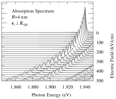
Figure 7: Absorption spectra for a CdSe nanocrystal at different electric field intensities. The light wave vector and its polarization $\mathbf{e}_{l}$ are perpendicular to the electric field.

Let us consider two simple configurations for photoluminescence experiments. First, the emitted light, with wave vector $\bm{\kappa}$, is recorded along the $\mathbf{E}_{QD}$ direction and its polarization vector $\mathbf{e}_{l}$ is parallel to $\mathbf{\hat{e}}_{x},$ (that is, $\mathbf{e}_{l}\parallel\mathbf{\hat{e}}_{x}\perp\mathbf{E}_{QD}$). In this case the dipole element $D_{x}=\mathbf{\hat{e}}_{x}\cdot\mathbf{D}_{\Psi,G}$ is not zero and, according to Table 1, the states with $M_{z}=\pm 1$ of the lowest excitonic level are optically active. Photoluminescence spectra should provide the Stark splitting presented in Fig. 2. Second, the emitted light is observed perpendicular to the field ($\bm{\kappa}\perp\mathbf{E}_{QD}$). Here, we have two choices for the light polarization, (i) $\mathbf{e}_{l}\parallel\mathbf{E}_{QD}$ or (ii) $\mathbf{e}_{l}\perp\mathbf{E}_{QD}$. In the case (i), $\mathbf{e}_{l}\parallel\mathbf{\hat{e}}_{z}\parallel\mathbf{\hat{e}}_{M_{z}=0}$ and the emitted light corresponds to the excitonic state II and the photoluminescence spectrum presents only one peak. In the configuration (ii), both excitonic states I and II are activated and the Stark splitting of Fig. 2 appears. The case (ii) is illustrated in Fig. 7 for the absorption spectra of a single QD at different electric fields. In the figure, the quenching of the absorption lines and the split of the 1s-1S_3/2 exciton peak as the electric field increases are clearly observed.

The above picture is slightly modified by the cubic anisotropy. At zero electric field, the 8-fold degenerate 1s-1S_3/2 excitons belong to the representations $\mathcal{D}^{-}_{1}$ ($M=1$) and $\mathcal{D}^{-}_{2}$ ($M=2$) of group $O(3)$. It is remarkable that the Coulomb interaction does not remove the degeneracy of $\mathcal{D}^{-}_{1}$ and $\mathcal{D}^{-}_{2}$, and neither does it for higher levels. According to the compatibility tables for groups $O(3)$ and $T_{d}$,Koster et al. (1963) $\mathcal{D}^{-}_{1}=\Gamma_{5}$ and $\mathcal{D}^{-}_{2}=\Gamma_{3}+\Gamma_{4}$. Hence, the $M=1$ triplet is not splitted. As only $\Gamma_{5}$ is dipole allowed, the selection rule $M=1$ remains valid for the ground exciton state. Only exciton states $n$s-$N$S_3/2 belong to $\mathcal{D}^{-}_{1}$ and are dipole allowed in the spherical approximation. The rest of the states, except $n$s-$N$P_1/2, split in different levels that include $\Gamma_{5}$ and should produce weak lines in the optical spectra. For non-zero electric field, the $O(3)$ symmetry is reduced to $C_{\infty v}$, and the irreducible representations correspond to the different values of $|M_{z}|$. The effect of the cubic terms depend upon the orientation of the crystal axes relative to the electric field. If $\mathbf{E}_{QD}$ is parallel to a 3-order axis, the symmetry is reduced to $C_{3v}$. Hence, the excitons with $M_{z}=0$ and $M_{z}=\pm 1$ belong to the $\Gamma_{1}$ and $\Gamma_{3}$ irreducible representations of $C_{3v}$, respectively, and are not modified by the symmetry reduction. Excitons with higher $|M_{z}|$ can split and give rise to weak optical transitions. If the electric field is not oriented along a 3-order axis, all the degeneracies are removed and additional transitions should appear. However, as the cubic anisotropy is induced fundamentally through the hole states, the splittings and intensities of the extra lines should be extremely small.

The fine structure that we have revealed can be modified by other effects present in real nanocrystals, such as shape asymmetry, crystal field (in wurtzite nanocrystals), and the electron-hole exchange interaction.Efros et al. (1996) These effects lead to a splitting pattern of the 8-fold lowest exciton into 5-levels, which is combined with the electric field-induced splitting. Non-adiabatic phonon-induced effectsFomin et al. (1998) and dielectric mismatch-induced modifications of the Coulomb interactionBanyai et al. (1992) contribute also to the magnitude of the splittings. For CdSe QDs with wurtzite structure the relative orientation of the crystallographic axes and the external electric field must have observable signatures in the optical spectra. These effects may be stronger than those produced by the cubic anisotropy. Since our approach ignores these effects our discussion is approximate.

In summary, we have studied the influence of the electric field on the electron and hole single particle states in CdSe nanocrystals, as well as on the exciton states and the optical properties. We have described the electric-field-induced quenching of the absorption and luminescence spectra and the importance of the exciton effects. We have found that the Coulomb interaction has a large influence on the strength of the optical transitions, even for small quantum dots. This fact is related to the penetration of electron wave function in the embedding medium, that partially breaks the strong confinement regime. Moreover, we have shown that for small QDs the dependence of the exciton binding energy upon the applied electric field is strongly reduced. For zero electric field we have reported very general expressions for the solutions of the 4$\times 4$ hole Hamiltonian in spherical QDs.

Appendix A Matrix elements of the Stark term

The Stark term in the electron effective mass Hamiltonian is a component of an irreducible spherical tensor of rank 1. The theorem of Wigner-Eckart and the reduction formulas for compound systems detailed in Ref. Brink and Satcher, 1968 allows us to write the matrix elements as

$$\left\langle n^{\prime}l^{\prime}f^{\prime}f_{z}^{\prime}\left||e|E_{QD}r\cos\theta\right|nlff_{z}\right\rangle$$ (19)

$$= (-1)^{f^{\prime}-f_{z}^{\prime}+3/2+f}|e|E_{QD}\sqrt{(2f^{\prime}+1)(2f+1)}$$

$$\times\left(\begin{array}[]{ccc}f^{\prime}&1&f\\ -f_{z}^{\prime}&0&f_{z}\end{array}\right)\left\{\begin{array}[]{ccc}f^{\prime}&f&1\\ l&l^{\prime}&1/2\end{array}\right\}\left(\begin{array}[]{ccc}l^{\prime}&1&l\\ 0&0&0\end{array}\right)$$

$$\times\sqrt{(2l^{\prime}+1)(2l+1)}\int R_{n^{\prime}l^{\prime}}(r)R_{nl}(r)r^{3}dr,$$

where the terms inside $\{\}$ and $()$ are the Wigner’s 6-j and 3-j symbols, respectively.

For the hole states we have found the expression

$$\left\langle N^{\prime}L^{\prime}F^{\prime}F_{z}^{\prime}\left|-|e|E_{QD}r\cos\theta\right|NLFF_{z}\right\rangle$$ (27)

$$= (-1)^{F^{\prime}-F_{z}^{\prime}+3/2+F}|e|E_{QD}\sqrt{(2F^{\prime}+1)(2F+1)}$$

$$\times\left(\begin{array}[]{ccc}F^{\prime}&1&F\\ -F_{z}^{\prime}&0&F_{z}\end{array}\right)\sum_{K,K^{\prime}}\left\{\begin{array}[]{ccc}F^{\prime}&F&1\\ K&K^{\prime}&3/2\end{array}\right\}\left(\begin{array}[]{ccc}K^{\prime}&1&K\\ 0&0&0\end{array}\right)$$

$$\times\sqrt{(2K^{\prime}+1)(2K+1)}\int R_{N^{\prime},K^{\prime}}^{(F^{\prime})}(r)R_{N,K}^{(F)}(r)r^{3}dr.$$

For the exciton states we found the expression

$$\left\langle n^{\prime}N^{\prime}l^{\prime}L^{\prime}f^{\prime}F^{\prime};M^{\prime}M_{z}^{\prime}\left||e|E_{QD}(r_{e}\cos\theta_{e}-r_{h}\cos\theta_{h})\right|nNlLfF;MM_{z}\right\rangle$$ (44)

$$= |e|E_{QD}(-1)^{M^{\prime}-M_{z}^{\prime}}\delta_{M_{z},M_{z}^{\prime}}\left(\begin{array}[]{ccc}M^{\prime}&1&M\\ -M_{z}^{\prime}&0&M_{z}\end{array}\right)\sqrt{(2M+1)(2M^{\prime}+1)}\Bigg{\{}\delta_{N,N^{\prime}}\delta_{L,L^{\prime}}\delta_{F,F^{\prime}}(-1)^{F+M+f+f^{\prime}+1/2}$$

$$\times\sqrt{(2f^{\prime}+1)(2f+1)(2l^{\prime}+1)(2l+1)}\left\{\begin{array}[]{ccc}f^{\prime}&f&1\\ l&l^{\prime}&1/2\end{array}\right\}\left\{\begin{array}[]{ccc}M^{\prime}&M&1\\ f&f^{\prime}&F\end{array}\right\}\left(\begin{array}[]{ccc}l^{\prime}&1&l\\ 0&0&0\end{array}\right)\int R_{n^{\prime}l^{\prime}}(r_{e})R_{nl}(r_{e})r_{e}^{3}dr_{e}$$

$$-\delta_{n,n^{\prime}}\delta_{l,l^{\prime}}\delta_{f,f^{\prime}}(-1)^{M^{\prime}+f+3/2+2F}\sqrt{(2F^{\prime}+1)(2F+1)}\sum_{K,K^{\prime}}\sqrt{(2K^{\prime}+1)(2K+1)}$$

$$\times\left\{\begin{array}[]{ccc}F^{\prime}&F&1\\ K&K^{\prime}&3/2\end{array}\right\}\left\{\begin{array}[]{ccc}M^{\prime}&M&1\\ F&F^{\prime}&f\end{array}\right\}\left(\begin{array}[]{ccc}K^{\prime}&1&K\\ 0&0&0\end{array}\right)\int R_{N^{\prime},K^{\prime}}^{(F^{\prime})}(r_{h})R_{N,K}^{(F)}(r_{h})r_{h}^{3}dr_{h}\Bigg{\}}.$$

References

- Mendez et al. (1982) E. E. Mendez, G. Bastard, L. L. Chang, L. Esaki, H. Morkoc, and R. Fischer, Phys. Rev. B 26, 7101 (1982).
- Miller et al. (1984) D. A. B. Miller, D. S. Chemla, T. C. Damen, A. C. Gossard, W. Wiegmann, T. H. Wood, and C. A. Burrus, Phys. Rev. Lett. 53, 2173 (1984).
- Kapteyn et al. (1999) C. M. A. Kapteyn, F. Heinrichsdorff, O. Stier, R. Heitz, M. Grundmann, N. D. Zakharov, D. Bimberg, and P. Werner, Phys. Rev. B 60, 14265 (1999).
- Miller et al. (1988) D. A. B. Miller, D. S. Chemla, and S. Schmitt-Rink, Appl. Phys. Lett. 52, 2154 (1988).
- Raymond et al. (1998) S. Raymond, J. P. Reynolds, J. L. Merz, S. Fafard, Y. Feng, and S. Charbonneau, Phys. Rev. B 58, R13415 (1998).
- Fry et al. (2000) P. W. Fry, I. E. Itskevich, D. J. Mowbray, M. S. Skolnick, J. J. Finley, J. A. Barker, E. P. O’Reilly, L. R. Wilson, I. A. Larkin, P. A. Maksym, et al., Phys. Rev. Lett. 84, 733 (2000).
- Yoffe (2001) A. D. Yoffe, Adv. Phys. 50, 1 (2001).
- Empedocles and Bawendi (1997) S. A. Empedocles and M. G. Bawendi, Science 278, 2114 (1997).
- Blanton et al. (1996) S. A. Blanton, M. A. Hines, and P. Guyot-Sionnest, Appl. Phys. Lett. 69, 3905 (1996).
- Viña et al. (1987) L. Viña, R. T. Collins, E. E. Mendez, and W. I. Wang, Phys. Rev. Lett. 58, 832 (1987).
- Bauer and Ando (1987) G. E. W. Bauer and T. Ando, Phys. Rev. Lett. 59, 601 (1987).
- Bauer and Ando (1988) G. E. W. Bauer and T. Ando, Phys. Rev. B 38, 6015 (1988).
- Canham (1990) L. T. Canham, Appl. Phys. Lett. 57, 1046 (1990).
- Wolkin et al. (1999) M. V. Wolkin, J. Jorne, P. M. Fauchet, G. Allan, and C. Delerue, Phys. Rev. Lett. 82, 197 (1999).
- Efros et al. (1996) A. L. Efros, M. Rosen, M. Kuno, M. Nirmal, D. J. Norris, and M. Bawendi, Phys. Rev. B 54, 4843 (1996).
- Casado and Trallero-Giner (1996) E. Casado and C. Trallero-Giner, Phys. Status Solidi B 196, 335 (1996).
- Wen et al. (1995) G. W. Wen, J. Y. Lin, H. X. Jiang, and Z. Chen, Phys. Rev. B 52, 5913 (1995).
- Baldereschi and Lipari (1973) A. Baldereschi and N. O. Lipari, Phys. Rev. B 8, 2697 (1973).
- Chang and Xia (1998) K. Chang and J.-B. Xia, J. Appl. Phys. 84, 1454 (1998).
- Menéndez-Proupin (2003) E. Menéndez-Proupin, J. Appl. Phys. (2003), submitted.
- Menéndez et al. (1997) E. Menéndez, C. Trallero-Giner, and M. Cardona, Phys. Status Solidi B 199, 81 (1997).
- Jackson (1962) J. D. Jackson, Classical Electrodynamics (Wiley, New York, 1962).
- Aggarwal (1974) L. R. Aggarwal, in Modulation Techniques, edited by P. K. Willardson and A. C. Beer (Academic, New York, 1974), vol. 9 of Semiconductors and Semimetals, p. 151.
- Brink and Satcher (1968) D. M. Brink and G. R. Satcher, Angular Momentum (Clarendon Press, Oxford, 1968).
- Laheld and Einevoll (1997) U. E. H. Laheld and G. T. Einevoll, Phys. Rev. B 55, 5184 (1997).
- Madelung (1986) O. Madelung, ed., Landolt-Börnstein Numerical Data and Functional Relationships in Science and Technology, vol. III/22 (Springer, Berlin, 1986).
- Hermann and Weisbuch (1977) C. Hermann and C. Weisbuch, Phys. Rev. B 15, 823 (1977).
- Menéndez-Proupin et al. (1999) E. Menéndez-Proupin, C. Trallero-Giner, and A. García-Cristobal, Phys. Rev. B 60, 5513 (1999).
- Xia (1989) J.-B. Xia, Phys. Rev. B 40, 8500 (1989).
- Efros (1992) A. L. Efros, Phys. Rev. B 46, 7448 (1992).
- Baldereschi and Lipari (1974) A. Baldereschi and N. O. Lipari, Phys. Rev. B 9, 1525 (1974).
- Koster et al. (1963) G. F. Koster, J. O. Dimmock, R. G. Wheeler, and H. Statz, Properties of the thirty-two point groups (M.I.T. Press, Cambridge, Massachusetts, 1963).
- Menéndez-Proupin and Cabo-Bisset (2002) E. Menéndez-Proupin and N. Cabo-Bisset, Phys. Rev. B 66, 085317 (2002).
- Kash et al. (1985) J. A. Kash, E. E. Mendez, and H. Morkoç, Appl. Phys. Lett. 46, 173 (1985).
- Miller and Gossard (1983) R. C. Miller and A. C. Gossard, Appl. Phys. Lett. 43, 954 (1983).
- Wang (2001) L.-W. Wang, J. Phys. Chem. B 105, 2360 (2001).
- Eychmüller (2000) A. Eychmüller, J. Phys. Chem. B 104, 6514 (2000).
- Tittel et al. (1997) J. Tittel, W. Göhde, F. Koberling, T. Basché, A. Kornowski, H. Weller, and A. Eychmüller, J. Phys. Chem. B 101, 3013 (1997).
- Shim et al. (2001) M. Shim, C. Wang, and P. Guyot-Sionnest, J. Phys. Chem. B 105, 2369 (2001).
- Rabani et al. (1999) E. Rabani, B. Hetényi, B. J. Berne, and L. E. Brus, J. Chem. Phys. 110, 5355 (1999).
- Fu (2002) H. Fu, Phys. Rev. B 65, 045320 (2002).
- Fomin et al. (1998) V. M. Fomin, V. N. Gladilin, J. T. Devreese, E. P. Pokatilov, S. N. Balaban, and S. N. Klimin, Phys. Rev. B 57, 2415 (1998).
- Banyai et al. (1992) L. Banyai, P. Gilliot, Y. Z. Hu, and S. W. Koch, Phys. Rev. B 45, 14136 (1992).