Linear scaling computation of the Fock matrix VII.
Periodic Density Functional Theory at the $\Gamma$-point.

Abstract

Linear scaling quantum chemical methods for Density Functional Theory are extended to the condensed phase at the $\Gamma$-point. For the two-electron Coulomb matrix, this is achieved with a tree-code algorithm for fast Coulomb summation [J. Chem. Phys. 106, 5526 (1997)], together with multipole representation of the crystal field [J. Chem. Phys. 107, 10131 (1997)]. A periodic version of the hierarchical cubature algorithm [J. Chem. Phys. 113, 10037 (2000)], which builds a telescoping adaptive grid for numerical integration of the exchange-correlation matrix, is shown to be efficient when the problem is posed as integration over the unit cell. Commonalities between the Coulomb and exchange-correlation algorithms are discussed, with an emphasis on achieving linear scaling through the use of modern data structures. With these developments, convergence of the $\Gamma$-point supercell approximation to the ${\bf k}$-space integration limit is demonstrated for MgO and NaCl. Linear scaling construction of the Fockian and control of error is demonstrated for RBLYP/6-21G* diamond up to 512 atoms.

Keywords: Self-consistent-field, linear-scaling, periodic systems, $\Gamma$-point, tree-code, Gaussian-orbital, adaptive grid, $k$-d trees

I INTRODUCTION

Quantum chemical methods that employ Gaussian-Type Atomic Orbitals (GTAOs) offer a number of advantages in materials science. First, because they are local basis functions, it is possible to achieve a linear scaling cost with system size for insulating systems. Secondly, almost all one- and two-electron integrals involving GTAOs are analytic, enabling the rapid evaluation of expectation values involving complicated operators that are often involved in the computation of response properties Honda et al. (1991); Helgaker and Taylor (1992); Stephens et al. (1994). The DALTON quantum chemical program Helgaker et al. (2001) is a premier example of this capability, offering a wide range of electric and magnetic molecular response properties. The ability to treat core-states analytically also opens the ability to go beyond the pseudopotential approximation in computation of relativistic effects with the four-component Dirac-Hartree-Fock Laerdahl et al. (1997); Grant and Quiney (2000) and Dirac-Kohn-Sham Yanai et al. (2001) theories. Perhaps most important though, the exact Hartree-Fock (HF) exchange may be computed efficiently with a GTAO basis set. In addition to providing a reference for correlated wavefunction methods, the exact HF exchange is central to hybrid HF/DFT models Gill et al. (1992); Becke (1993); Barone et al. (1996); Adamo et al. (1999). The use of hybrid methods in the condensed phase, pioneered by the CRYSTAL group Saunders et al. (1998), has proven to be a useful improvement beyond the generalized gradient approximation for a number of properties, including bulk geometries, electronic properties Bredow and Gerson (2000); Muscat et al. (2001) and absorption energies Baranek et al. (2001); Wander and Harrison (2001).

Recently, we have developed linear scaling quantum chemical methods for gas phase Density Functional Theory (DFT), including computation of the Coulomb matrix ${\bf J}$ Challacombe and Schwegler (1997) and the exchange-correlation matrix $\bf K_{\rm xc}$ Challacombe (2000). In this contribution, these linear scaling methods are extended to periodic boundary conditions at the $\Gamma$-point.

With periodic linear scaling quantum chemical algorithms, it is possible to begin bridging the gap between methods developed for small molecule chemistry and large scale problems in the solid state. Together with the results presented here, ${\cal O}(N)$ methods for solving the Self-Consistent-Field equations Niklasson (2002); Niklasson et al. (2003) and linear scaling algorithms for computing the periodic HF exchange Tymczak et al. (2004), it is now possible to perform condensed phase HF/DFT calculations on systems larger than 500 atoms with a single processor. In addition, with the advent of linear scaling density matrix perturbation theory Niklasson and Challacombe (2004); Weber et al. (2004), well developed quantum chemical methods for the analytic computation of response properties may be brought to bear on large solid state problems.

This paper is organized as follows: In Section II, periodic boundary conditions and the $\Gamma$-point approximation are introduced. Next, in Section III, the relationship between the numerical error estimates and data structures that underly the fast linear scaling algorithms for computation of the Coulomb and exchange-correlation matrix are outlined. In Section IV, we extend previous work on the Niboer and De Wette Nijboer and De Wette (1957, 1958) lattice sum method to linear scaling computation of quantum Coulomb sums and tin-foil boundaries. Then, in Section V, ${\cal O}(N)$ methods for computing the GTAO-based exchange-correlation matrix are presented. In Section VI.1 we discuss the implementation of these developments in the MondoSCF Challacombe et al. (2001) suite of linear scaling quantum chemistry codes. In Section VI.2, comparison of the $\Gamma$-point results is made with those obtained with CRYSTAL98 using ${\bf k}$-space integration for NaCl and MgO. Next, in Section VI.3, linear scaling is demonstrated for construction of the diamond Fock matrix at the RBLYP/6-21G* level of theory. Finally, in Section VII, we present our conclusions.

II periodic boundary conditions, linear scaling and basis sets

In the conventional implementations of periodic boundary conditions, the Bloch functions

$$\psi^{\bf k}_{a}({\bf r})=\sum_{\bf R}e^{i{\bf k}\cdot{\bf R}}\phi_{a}({\bf r}-{\bf R}),$$ (1)

are often constructed from non-orthogonal functions local to the unit cell (UC). Here, the local function $\phi_{a}$ is a Gaussian-Type Atomic Orbital (GTAO) centered on atom A, while the sum on R runs over the Bravais lattice defined by integer translates of the primitive lattice vectors a, b and c. These Bloch functions (crystal orbitals) yield all possible translational symmetries through variation of the reciprocal lattice vector k. Programs such as CRYSTAL98 perform a careful sampling of reciprocal space to achieve an accurate description of the periodic system. An alternative approach to including these important symmetries is to set ${\bf k}=0$, and then use a larger supercell created through replication and translation of the primitive unit cell. This is the supercell $\Gamma$-point approximation, used primarily for the study of defects and vacancies rather than as a replacement for ${\bf k}$-space integration.

In this contribution, ${\cal O}(N)$ algorithms are developed specifically for the the $\Gamma$-point approximation, allowing the use of large supercells in the case of high symmetry, as well as large primary cells in the case of disordered systems. While ${\bf k}$ dependence is avoided, lattice summation and formal integration over the unit cell volume, $V_{\rm UC}$, are retained. At first sight this would seem to make matrix construction quite different than in the gas phase, where integrals are typically taken over all space, $V_{\infty}$. Thus, elements of the gas phase overlap matrix,

$$S_{ab}=\int_{V_{\infty}}\,d{\mathbf{r}}\,\phi_{a}({\mathbf{r}})\phi_{b}({\mathbf{r}})\,,$$ (2)

become

$$S_{ab}=\sum_{\mathbf{R},\mathbf{R}^{\prime}}\int_{V_{\rm UC}}\,d{\mathbf{r}}\,\phi_{a}({\mathbf{r}+\mathbf{R}})\phi_{b}({\mathbf{r}+\mathbf{R}^{\prime}})$$ (3)

in the periodic $\Gamma$-point regime. However, this formalism can be brought into a form more closely related to its quantum chemical counterpart via the transformation,

$$\sum_{\bf R}\int_{V_{\rm UC}}d{\bf r}f({\bf r+R})\rightarrow\int_{V_{\infty}}d{\bf r}f({\bf r}),$$ (4)

allowing use of conventional analytic integral technologies. For example, elements of the periodic overlap matrix become

$$S_{ab}=\sum_{\mathbf{R}}\int_{V_{\infty}}\,d{\mathbf{r}}\,\phi_{a}({\mathbf{r}})\phi_{b}({\mathbf{r}+\mathbf{R}}).$$ (5)

For compactness of notation, let us define the intermediate basis function products (distributions) $\rho_{ab}({\mathbf{r}})=\sum_{\mathbf{R}\mathbf{R}^{\prime}}\phi_{a}({\mathbf{r}+\mathbf{R}})\phi_{b}({\mathbf{r}+\mathbf{R}^{\prime}})$ associated with integration over $V_{\rm UC}$ and the corresponding distributions $\rho_{ab}^{\scriptscriptstyle\infty}({\mathbf{r}})=\sum_{\mathbf{R}}\phi_{a}({\mathbf{r}})\phi_{b}({\mathbf{r}+\mathbf{R}})$ associated with integration over $V_{\infty}$. We likewise define the electron density $\rho({\mathbf{r}})=\sum_{ab}P_{ab}\rho_{ab}({\mathbf{r}})$ associated with integration over $V_{\rm UC}$ and the corresponding density $\rho^{\scriptscriptstyle\infty}({\bf{r}})=\sum_{ab}P_{ab}\rho_{ab}^{\scriptscriptstyle\infty}({\mathbf{r}})$ associated with integration over $V_{\infty}$, where $P_{ab}$ is the one-electron reduced density matrix. In this convention, $V_{\infty}$ is the default volume of integration, and elements of the periodic overlap matrix are expressed simply as $S_{ab}=\int d{\mathbf{r}}\,\rho^{\scriptscriptstyle\infty}_{ab}({\mathbf{r}})$, while the electron count is $N_{\rm el}=\int d{\mathbf{r}}\,\rho^{\scriptscriptstyle\infty}({\mathbf{r}})$.

It is worth noting that the complexity of $\rho^{\scriptscriptstyle\infty}$ is ${\cal O}(N)$, due to the exponential prefactor $e^{-\chi_{ab}({\bf A}-{\bf B}-{\bf R})^{2}}$ that enters each term in the sum over A, B and R. Thus, $N$-scaling may be achieved a priori with a simple distance test. However, for small exponents, care must be exercised in truncation of periodic sums to avoid overlap matrices that are not positive definite. While these situations can often be ameliorated with a tighter distance neglect criteria, they are typically a symptom of near linear dependence, often due to the use of basis sets designed for gas phase calculations in conjunction with small unit cells.

These considerations and others are discussed by Towler in an excellent overview of Gaussian basis sets for the condensed phase Towler (2000). Also, there are at least two (albeit related) libraries Dovesi et al. (2003); Towler (1998) of Gaussian basis sets appropriate for materials at standard densities. For high densities though, these basis sets may still encounter problems with linear dependence and sensitivity to truncation. One solution to this problem, suggested by Grüneich and Hess Grüneich and Hess (1998) for even tempered basis sets, is to scale the exponents by the inverse square of the lattice constant. In many cases though, especially for large systems, standard quantum chemical basis sets work well.

III data structures and error estimates

Both the Quantum Chemical Tree-Code (QCTC) Challacombe and Schwegler (1997) for computing the Coulomb matrix and Hierarchical Cubature (HiCu) Challacombe (2000) for computing the Exchange-Correlation matrix are fast ${\cal O}(N{\rm lg}N)$ algorithms whose performance is coupled to underlying data structures and error estimates. It is important to understand some of these particulars first, before addressing their extension to periodic boundary conditions. Also, the current version of QCTC is quite different from previous descriptions, and deserves some introduction.

Both QCTC and HiCu are homeomorphic, involving $k$-d tree representation of the density. In our implementations, $k$-d trees are doubly linked lists with axis aligned bounding boxes (AABBs) delimiting the spatial extent of each node and its children. This scheme is similar to well developed technologies for ray tracing and data base searches, allowing fast ${\cal O}({\rm lg}N)$ range queries of overlapping components through AABB intersection tests Gomez (1999). In the case of QCTC, this fast look up constitutes the penetration acceptability criterion (PAC) which identifies spatial clusters or agglomerations, $\rho_{Q}$, of the density that may be accurately represented via a multipole approximation due to the absence of charge-charge penetration effects.

For accepted clusters a second test, the multipole acceptability criterion (MAC), is performed to check translation errors in the multipole expansion. This second test is critical to the overall accuracy of the Coulomb matrix build. We have recently developed a new MAC in Ref. [Tymczak and Challacombe, 2003] that has several advantages. First, it takes into account the magnitude or weight of the distribution within the cluster. Second, it correctly takes into account the angular symmetry of the primitive Gaussian distributions. Third, and most important, it is always an exact bound to the translation error.

For each primitive bra distribution $\rho_{ab}$, a fast range query is performed on the $k$-d tree representation of the total density, leading to an on the fly partition of near-field (NF) and far-field (FF) interactions in construction of the gas phase Coulomb matrix which may be written

$$J_{ab} = \sum_{Q\in\rm FF}\sum_{l}(-1)^{l}\sum_{m}O^{l}_{m}[\rho_{ab}]\sum_{l^{\prime}}\sum_{m^{\prime}}M^{l+l^{\prime}}_{m+m^{\prime}}O^{l^{\prime}}_{m^{\prime}}[\rho_{Q}]$$ (6)

$$+ \sum_{q\in\rm NF}\int d{\bf r}\int d{\bf r^{\prime}}\rho_{ab}({\bf r})\left|{\bf r}-{\bf r^{\prime}}\right|^{-1}\rho_{q}({\bf r})\,,$$

where $M^{l}_{m}$ is the irregular solid harmonic interaction tensor, $O^{l}_{m}[f]=\int d{\bf r}O^{l}_{m}({\bf r})f({\bf r})$ is a moment of the regular solid harmonic, $Q$ runs over the highest possible nodes in the density-tree consistent with the PAC and MAC, and $q$ runs on leftover near-field primitive distributions in the density. See Refs. [Challacombe and Schwegler, 1997; Challacombe et al., 1997] for further details on this representation.

A fundamental difference between QCTC and FMM based methods is that QCTC pushes the near/far-field partition to the limit, employing the PAC and MAC best case error estimates to resolve individual primitive distributions. On the other hand, FMM based methods employ static, worst case error estimates. While recurring down the density tree to the level of individual primitives precludes well developed technologies for the integral evaluation of contracted functions, it accelerates the onset of linear scaling through early clustering.

The Quantum Chemical Tree Code generally employs the total density, which simplifies the code, allows electrostatic screening in MAC error estimates and provides charge neutrality, an essential feature for periodic calculations. Thus, the Coulomb matrix employed here includes the electron-nuclear terms; ${\bf J}\equiv{\bf J}_{\rm ee}+{\bf V}_{\rm en}$.

In the case of HiCu, two separate $k$-d tree structures are used. The rho-tree holds the electron density, while the cube-tree contains a hierarchical grid for integration of the exchange-correlation potential. Each node of the cube-tree is composed of a Cartesian non-product integration rule with the grid points enclosed by it’s AABB. The cube-tree is constructed iteratively through recursive bisection of the primary volume (the root AABB), using exact error bounds to achieve arbitrary precision of the integrated density and its gradients. As the cube-tree is extended, AABB intersection tests are performed while traversing the rho-tree, avoiding parts of the density that do not overlap with that portion of the grid. Upon construction of the grid, the reverse procedure is carried out; for each primitive distribution, the cube-tree is walked selecting only overlapping portions of the grid via the AABB intersection test.

For both of these fast algorithms, the trade off between efficiency and accuracy is controlled by the AABB, which in turn depends on the the extent or range $R_{q}$ of a primitive Gaussian distribution $\rho_{q}$, beyond which it is assumed to be negligible. Of course, negligible depends on the use to which the distribution is put, as will become obvious in the following.

Both HiCu and QCTC employ the Hermite Gaussian representation of distributions Ahmadi and Almlöf (1995)

$$\rho_{q}({\bf r})=\sum_{lmn}d_{lmn}\Lambda^{q}_{lmn}({\bf r}),$$ (7)

where

$$\Lambda^{q}_{lmn}({\bf r})=\frac{\partial^{l+m+n}}{\partial Q^{l}_{x}\partial Q^{m}_{y}\partial Q^{n}_{z}}e^{-\zeta_{q}({\bf r}-{\bf Q})^{2}}.$$ (8)

This representation provides an intermediate form into which elements of the density matrix may be folded, and allows the use of McMurchie-Davidson recurrence relations McMurchie and Davidson (1978) in analytic integral evaluation and density evaluation. For this form, Cramer’s inequality Hille (1926) provides a bound for the behavior of a Hermite-Gaussian distribution:

$$\rho_{q}({\bf r})\leq C_{q}e^{-\widetilde{\zeta}_{q}({\bf r-Q})^{2}},$$ (9)

where

$$C_{q}=\sum_{lmn}\left|d_{lmn}\right|K^{3}\left[2^{l+m+n}~{}l!m!n!~{}\zeta^{l+m+n}_{q}\right]^{1/2},$$ (10)

the constant $K=1.09$, and

$$\widetilde{\zeta}_{q}=\begin{cases}\zeta_{q}&l+m+n=0\\ \frac{1}{2}\zeta_{q}&{\rm otherwise.}\end{cases}$$ (11)

The overlap extent $R^{\rm o}_{q}$ is the value beyond which numerical evaluation of the distribution $\rho_{q}$ yields a value less than $\tau$;

$$C_{q}e^{-\widetilde{\zeta}_{q}(R^{\rm o}_{q})^{2}}=\tau.$$ (12)

For QCTC, errors in the electrostatic potential due to penetration errors must be considered. For this purpose, the penetration extent $R^{\rm p}_{q}$ is introduced, satisfying the equation

$$C_{q}\int\left[\left(\pi/{\widetilde{\zeta}_{q}}\right)^{3/2}\delta({r})-e^{-\widetilde{\zeta}_{q}{r}^{2}}\right]\left|{r}-{R^{\rm p}_{q}}\right|^{-1}{\rm d}r=\tau.$$ (13)

In both HiCu and QCTC, the density-tree is constructed by recursively splitting the largest box dimension, until each primitive has been resolved. Then the primitive AABBs are computed from their extents and merged recursively back up the tree. For HiCu, this is all there is to it, but for QCTC multipole moments are also translated to a common center and recursively merged up the tree. Also, when computing matrix elements of $\bf J$, the primitive bra AABB is computed with $R^{\rm o}_{q}$, while the $R^{\rm p}_{q}$ are used to construct AABBs of the density-tree.

In Fig. 1, differences between the penetration and overlap extent are shown for a diffuse $s$-type Gaussian. For large extents, such as those encountered in a static FMM-type error bound, the two extents behave in a similar way. However, with aggressive use of the multipole approximation as in QCTC, the distinction becomes critical.

Figure 1: Behavior of the overlap extent $R^{o}$ and the penetration extent $R^{p}$ as a function of $\tau/C_{q}$ for an $s$-type Gaussian with exponent $\zeta=1$. For small $C_{q}$ (occurring for example due to a large atom-atom separation and/or small density matrix prefactor), $R^{o}$ goes to zero at the origin and its distribution is eliminated, while $R^{p}$ goes slowly to zero due to the Coulomb singularity.

IV Periodic Quantum Coulomb Sums

In the $\Gamma$-point approximation, elements of the periodic Coulomb matrix are

$$J_{ab} = \int_{V_{\rm UC}}d{\mathbf{r}}\int d{\mathbf{r}^{\prime}}{\rho_{ab}\left({\mathbf{r}}\right){\left|\mathbf{r}-\mathbf{r}^{\prime}\right|}^{-1}\rho_{\rm tot}\left(\mathbf{r}^{\prime}\right)}$$

$$= \sum_{\mathbf{R}}\int\int d{\mathbf{r}}\,d{\mathbf{r}^{\prime}}{\rho_{ab}^{\scriptscriptstyle\infty}\left({\mathbf{r}}\right){\left|\mathbf{r}-\mathbf{r}^{\prime}\right|}^{-1}\rho^{\scriptscriptstyle\infty}_{\rm tot}\left({\mathbf{r}^{\prime}}+{\mathbf{R}}\right)}$$

where $\rho_{\rm tot}$ is the total, periodic density including both electronic and nuclear terms. These integrals involve infinite summation over the lattice vectors ${\bf R}$, and must be handled with care. There are at least two main approaches to handling this summation: Multipole expansion of the Ewald potential or Ewald-like summation of the multipole expansion. Expansion of the Ewald potential yields tin foil (TF) boundary conditions, requires reciprocal and real space summation with every ${\bf J}$ build, and scales as $O(N^{3/2})$. An alternative is the Ewald-like summation of the multipole interaction tensor, which was first described by Nijboer and De Wette (NDW) Nijboer and De Wette (1957, 1958) and later reviewed and extended by Challacombe, White and Head-Gordon Challacombe et al. (1997) to lattice summation of the irregular solid harmonic multipole interaction tensor. This Ewald-like summation is taken over the periodic far field, $V_{\rm PFF}$, and is equivalent to a direct lattice summation (not a true Ewald sum) excluding an inner region, $V_{\rm In}$, surrounding the unit cell. This inner region has been subtracted to avoid penetration errors and to guarantee convergence of the multipole expansion. With the summed interaction tensors cheaply precomputed and reused, the cost of Coulomb summation over the PFF scales as as ${\cal O}(Np^{2})$, where $p$ is the order of the multipole expansion. With this partition, the $N$-scaling periodic quantum Coulomb sums involve the contributions

$${\bf J}={\bf J}^{\rm In}+{\bf J}^{\rm PFF}+{\bf J}^{\rm TF}\,,$$ (15)

corresponding to the three separate regions shown in Fig. 2. Here, ${\bf J}^{\rm In}$ is computed using the fast ${\cal O}(N{\rm lg}N)$ QCTC algorithm outlined previously in Section III. Construction of ${\bf J}^{\rm PFF}$ will be developed in the following section, while in Section IV.2 the term ${\bf J}^{\rm TF}$, necessary to introduce tin-foil boundary conditions, is detailed.

Figure 2: Schematic of the regions contributing to $N$-scaling summation of the Coulomb matrix. The inner cells that make up $V_{\rm In}$ provide a buffer region that guarantees convergence of the multipole expansion of Coulomb interactions between the unit cell and all cells in $V_{\rm PFF}$. The periodic far-field region, $V_{\rm PFF}$, is the spherically ordered lattice extending to infinity but excluding $V_{\rm In}$. For large cells and/or high order multipole expansions, $V_{\rm In}$ includes just the unit cell’s 27 nearest neighbors. In FMM notation this corresponds to ws=1. However, for smaller cells and/or lower order multipole expansions, $V_{\rm In}$ tends to a spherical distribution of cells surrounding the unit cell. Direct summation over $V_{\rm PFF}$ leads to charges at the infinite surface $S_{\infty}$, which must be be canceled by tin-foil (conducting) boundary conditions to achieve equivalence with Ewald summation.

IV.1 The Periodic Far Field

By construction, the periodic far field (PFF) term in the Coulomb matrix,

$$J_{ab}^{\rm PFF}=\sum_{{\bf R}\in{\rm PFF}}\int\int d{\bf r}d{\bf r^{\prime}}\rho^{\infty}_{ab}({\bf r}){\left|{\bf r}-{\bf r^{\prime}}+{\bf R}\right|}^{-1}\rho^{\infty}_{\rm tot}({\bf r^{\prime}}),$$ (16)

involves charge distributions that are well separated with respect to both penetration and the convergence of multipole expansion errors, as outlined in Fig. 2 and discussed in the following.

With these conditions, and assuming the unit cell is centered at the origin, the bipolar multipole expansion employing the regular and irregular solid harmonics, $O^{l}_{m}$ and $M^{l}_{m}$ respectively is

$${|{\bf r}-{\bf r}^{\prime}+{\bf R}|}^{-1} \approx \sum^{p}_{l=0}(-1)^{l}\,\sum^{p}_{l^{\prime}=0}\Bigl{[}$$

$$\sum^{l}_{m=-l}\,\sum^{l^{\prime}}_{m=-l^{\prime}}O^{m}_{l}({\bf r})\,M^{m+m^{\prime}}_{l+l^{\prime}}({\bf R})\,O^{m^{\prime}}_{l^{\prime}}({\bf r}^{\prime})\Bigr{]}\,.$$

Inserting Eq. (IV.1) into into Eq. (16) yields

$$J_{ab}^{\rm PFF} = \sum_{{\bf R}\in{\rm PFF}}\sum^{p}_{l=0}(-1)^{l}\,\sum^{p}_{l^{\prime}=0}\sum^{l}_{m=-l}\Bigl{(}$$

$$\sum^{l^{\prime}}_{m=-l^{\prime}}O_{l}^{m}\left[\rho^{\infty}_{ab}\right]\,M^{m+m^{\prime}}_{l+l^{\prime}}({\bf R})\,O_{l^{\prime}}^{m^{\prime}}\left[\rho^{\infty}_{\rm tot}\right]\Bigr{)}\,.$$

This expression decouples the complexity of $\rho^{\infty}_{ab}$ from $\rho^{\infty}_{\rm tot}$ through the precomputed multipole moments $O_{l}^{m}\left[\rho^{\infty}_{ab}\right]=\int d\mathbf{r}\,{O}_{l}^{m}\left(\mathbf{r}\right)\,\rho^{\infty}_{ab}\left(\mathbf{r}\right)$ and $O_{l}^{m}\left[\rho^{\infty}_{\rm tot}\right]=\int d\mathbf{r}\,{O}_{l}^{m}\left(\mathbf{r}\right)\,\rho^{\infty}_{\rm tot}\left(\mathbf{r}\right)$. Following Nijboer and De Wette Nijboer and De Wette (1957, 1958); Challacombe et al. (1997), we introduce the effective multipole interaction tensor

$${\cal M}^{m}_{l}=\sum_{{\bf R}\in V_{\rm PFF}}M^{m}_{l}({\bf R})\;,$$ (19)

which can be efficiently computed on the fly for each new lattice, both to high accuracy and to high order (large $p$) using the new methods detailed in Appendix A. Note that this is a direct sum of the interaction tensor, and is not equivalent to Ewald summation. Nevertheless, with this simplification, the ${\cal O}(p^{2}N)$ working equation

$$J_{ab}^{\rm PFF}=\sum^{p}_{l=0}\sum^{l}_{m=-l}O_{l}^{m}\left[\rho^{\infty}_{ab}\right]{\cal J}^{m}_{l}\;,$$ (20)

is obtained, where the intermediate tensor

$${\cal J}^{l}_{m}=(-1)^{l}\sum^{p}_{l^{\prime}=0}\sum^{l^{\prime}}_{m=-l^{\prime}}{\cal M}^{m+m^{\prime}}_{l+l^{\prime}}O_{l^{\prime}}^{m^{\prime}}\left[\rho^{\infty}_{\rm tot}\right]$$ (21)

is cheaply precomputed at the start of each Coulomb build.

Because Eq. (20) is inexpensive, our strategy is to define a minimal buffer region, $V_{\rm In}$, sufficient to control penetration errors, subtracting effort from the computation of $J^{\rm In}$ via QCTC and replacing it with cheaper, multipole work in the computation of $J^{\rm PFF}$. To this end, a fixed inner region $V_{\rm In}$ is constructed from neighboring cells that have simple Gaussian overlap with the unit cell, defined by the radius $R^{o}$. As explained in Section III, for the relatively large distances considered at this level the differences between the penetration and overlap extent are negligible. With $V_{\rm In}$ fixed, the precision of ${\bf J}^{\rm PFF}$ is controlled entirely by the expansion order $p$. In general $p$ will be much higher than the expansion order ($\sim 5$) employed by QCTC in computation of ${\bf J}^{\rm In}$. With QCTC accuracy is controlled on the fly by the MAC and PAC, establishing a dynamic near/far-field partition, while computation of ${\bf J}^{\rm PFF}$ involves a static, worst-case error dominated by the multipole expansion. This static error is controlled by using the FMM-like error bound,

$$\frac{2^{p}{\cal C}^{2}\,{d}_{\rm max}^{p+1}}{({R}^{o})^{p+1}\left|{R}^{o}-2\,{d}_{\rm max}\right|}\leq\tau_{\rm\scriptscriptstyle MAC}\;,$$ (22)

to set the appropriate expansion order $p$. In Eq. (22), $d_{\rm max}$ is the maximum translational distance, ${\cal C}$ is the asymptotic Unsöld weight of the total density and $\tau_{\rm\scriptscriptstyle MAC}$ is the threshold controlling the translation errors. See Ref. Tymczak and Challacombe, 2003 for development of this expression and further explanation of these parameters.

IV.2 Tin-Foil Boundary Conditions

The surface charges created by direct summation over $V_{\rm PFF}$ must be canceled to achieve equivalence with Ewald summation. Achieving this equivalence is more than semantic, since without tin-foil boundary conditions matrix elements lack translational invariance and often incur dramatic charge sloshing instabilities. The correction is strongly dependent on ordering of the direct sum; as the Nijboer and De Wette method corresponds to spherical summation due to symmetry of the real/reciprocal space partition, the appropriate correction is Redlack and Grindlay (1972)

$$\Phi_{\rm Ew}\left(\mathbf{r}\right)=\Phi_{\rm SS}\left(\mathbf{r}\right)+\frac{2\pi}{3V_{\rm UC}}\left(Q-2\,{\bf r}\cdot\mathbf{D}\right),$$ (23)

where ${\bf D}$ is the system dipole moment, $Q$ is trace of the system quadrupole and we have assumed origin centering, The tin-foil correction to the Coulomb matrix is then

$$J_{ab}^{TF}=\frac{2\pi}{3V_{\rm UC}}\left(Q\,S_{ab}-2\,\mathbf{d}_{ab}\cdot\mathbf{D}\right)$$ (24)

with $S_{ab}$ an element of the overlap matrix, and ${\bf d}_{ab}$ the dipole moment of the distribution $\rho^{\infty}_{ab}$.

Figure 3: Transformation between the unit cell with volume $V_{\rm UC}$ (described by the primitive lattice vectors a, b and c) and the rectangular integration volume $V_{\Box}$ employed by HiCu.

V Periodic exchange-correlation

The HiCu algorithm is ideally suited for periodic boundary conditions, as the unit-cell $V_{\rm UC}$ can be simply transformed into an equivalent rectangular integration domain $V_{\Box}$ that is the cube-tree’s AABB. These volumes, shown in Fig. 3, are equivalent due to full periodicity of both distributions and density. The integration is then simply

$$K^{\rm xc}_{ab}=\int_{V_{\Box}}\,d\mathbf{r}\,\rho_{ab}({\bf r})v_{\rm\scriptscriptstyle xc}\left[\rho;{\bf r}\right]$$ (25)

This approach should be contrasted with more conventional quantum chemical methods for computing the exchange-correlation matrix, involving the “Becke weights” Becke (1988a), which demand numerical integration over $V_{\infty}$.

While we have written Eq. 25 in terms of the exchange-correlation potential for simplicity, in practice HiCu employs the Pople, Gill and Johnson formulation Pople et al. (1992); Challacombe (2000).

Because the distributions and density both involve a double sum over lattice vectors, there will be a large number of atom-atom pairs that do not overlap with $V_{\Box}$. A similar situation is encountered in the gas phase for parallel versions of HiCu Gan and Challacombe (2003), where each processor has a small, local cube-tree that may overlap only a few of the many possible atom-atom pairs. The solution to this problem again comes from the ray tracing literature, in the form of a modified ray-AABB Gomez (1999) and sphere-AABB test Glassner (1990). The ray-AABB test has been modified into a cylinder-AABB test, where the radius of the cylinder is a maximal overlap extent of the atom-atom pair. In the case of a same center atom-atom pair, it is of course more appropriate to employ a sphere-AABB test. In both cases, overlap between the HiCu integration volume and atom-atom pairs is established with a negligible prefactor when using these tests.

Table 1: Comparison of CRYSTAL98 and MondoSCF $\Gamma$-point calculations on NaCl at the RBLYP/8-511/8-631G level of theory.

Program	$N_{\rm at}$	Energy (au)	Energy/$N_{\rm at}$
MondoSCF	$2^{f}$	-622.39101	-311.19551
CRYSTAL98	$2^{f}$	-622.39114	-311.19557
MondoSCF	$8^{g}$	-2490.0016	-311.25020
CRYSTAL98	$8^{g}$	-2490.0013	-311.25016
fTriclinic
gCubic

Table 2: Convergence of the $\Gamma$-point super-cell approximation for NaCl, computed with MondoSCF at the RLDA/STO-3G level of theory.

Program	$N_{\rm at}$	Energy (au)	Energy/$N_{\rm at}$
MondoSCF	2f	-610.97536	-305.48768
	8g	-2444.3584	-305.54480
	16f	-4888.7002	-305.54377
	54f	-16499.490	-305.54611
	64g	-19554.956	-305.54618
	128f	-39109.912	-305.54618
	216g	-65997.977	-305.54619
CRYSTAL98h	2f	-611.09228	-305.54614
fTriclinic
gCubic
${}^{h}6\times 6\times 6$ $\bf k$-space grid.

Table 3: Convergence of the $\Gamma$-point super-cell approximation for MgO, computed with MondoSCF at the RBLYP/8-61G/8-51G level of theory.

Program	$N_{\rm at}$	Energy (au)	Energy/$N_{\rm at}$
MondoSCF	2f	-275.09097	-137.54548
	8g	-1101.7295	-137.71618
	16f	-2203.6904	-137.73065
	54f	-7437.7989	-137.73702
	64g	-8815.2131	-137.73771
	128f	-17630.430	-137.73774
	216g	-29751.352	-137.73774
CRYSTAL98h	2f	-275.47547	-137.73774
fTriclinic
gCubic
${}^{h}6\times 6\times 6$ $\bf k$-space grid.

Table 4: Convergence of the $\Gamma$-point super-cell approximation for diamond, computed with MondoSCF at the RBLYP/6-21G* level of theory.

$N_{\rm at}$	Energy (au)	Energy/$N_{\rm at}$
8	-303.989	-37.9986
16	-608.667	-38.0417
32	-1218.02	-38.0632
64	-2436.28	-38.0669
96	-3654.59	-38.0687
144	-5482.04	-38.0697
216	-8223.10	-38.0699
288	-10964.1	-38.0700
384	-14618.9	-38.0700

VI Results

VI.1 Implementation

All developments were implemented in a serial version of MondoSCF v1.0$\alpha$9 Challacombe et al. (2001), a suite of linear scaling Quantum Chemistry code. The code was compiled using the Portland Group F90 compiler pgf90 v4.2 The Portland Group (2002) with the -O1 -tp athlon options and with the Gnu C compiler gcc v3.2.2 using the -O1 flag. All calculations were carried out on a 1.6GHz AMD Athlon running RedHat Linuxv9.0 Redhat (2004).

Thresholds controlling the cost to accuracy ratio of HiCu and QCTC are set by the accuracy levels LOOSE, GOOD and TIGHT, which have been empirically chosen to deliver 4-5, 6-7 and 8-9 digits, respectively, of relative accuracy in the energy. Values of these thresholds are listed in Appendix B of Ref. [Tymczak et al., 2004]. The unmodified two-electron threshold $\tau_{\rm\scriptscriptstyle 2E}$ sets the overlap extent $R^{o}_{p}$ in Eq. (12) and the penetration extent $R^{p}_{q}$ in Eq. (13), both of which control the PAC. As explained in Ref. [Tymczak and Challacombe, 2003], the threshold $\tau_{\rm\scriptscriptstyle MAC}$ controlling the MAC is set as $\tau_{\rm\scriptscriptstyle MAC}=10^{2}\tau_{\rm\scriptscriptstyle 2E}$. The HiCu threshold $\tau_{\rm\scriptscriptstyle HICU}$ likewise sets two sub-thresholds. The overlap extent $R^{o}_{p}$ in Eq. (12), defining accuracy of the density on the grid, is set using $10^{-1}\tau_{\rm\scriptscriptstyle HICU}$ ($\tau_{\rho}$ in Ref. [Challacombe, 2000]). The target relative error defining accuracy of the HiCu grid is just $\tau_{\rm\scriptscriptstyle HICU}$ ($\tau_{r}$ in Ref. [Challacombe, 2000]). It should be pointed out that of all the thresholding schemes, those governing HiCu are the least conservative; it is a simple (and not too expensive) matter to simply tighten the HiCu threshold if intermediate accuracies are required.

The multipole interaction and contraction code used by QCTC in the near/far-field partition has been highly optimized by symbolic manipulation and factorization, using real arithmetic and expansions through 7’th order in the calculation of ${\bf J}^{\rm In}$. The computation of ${\bf J}^{\rm PFF}$ employs a general code for multipole contraction, allowing expansion through $p=64$. Eigensolution of the self-consistent-field equations has been used throughout, with the corresponding matrix and distribution thresholds given Appendix B of Ref. [Tymczak et al., 2004]. All calculations were performed with $C_{1}$ (no) symmetry, and all results are reported in atomic units.

Figure 4: Error in the Coulomb energy computed with the Nijboer and De Wette scheme relative to true Ewald summation. Shown is the error in the Coulomb energy versus $p$ with one (ws=1) and two (ws=2) layers of cells in $V_{\rm PFF}$ for a periodic system of 64 classical water molecules.

VI.2 Validation

The ability of our implementation to reproduce true Ewald summation is shown in Fig. 4 for a periodic system of 64 classical water molecules. Note that with both the Ewald sum and the Nijboer and De Wette approach, ordering the real and reciprocal space sums is critical; high order agreement is achieved only when the summation proceeds from the smallest to the largest terms.

The use of Cartesian Gaussian basis sets in many cases allows direct numerical comparison of different programs, at least to within the approximations, grids, etc peculiar to a code. Here, we make connection with the preeminent Gaussian orbital program for periodic calculations, CRYSTAL98 Saunders et al. (1998). Calculations have been carried out largely with basis sets optimized for the condensed phaseDovesi et al. (2003), which tend to have less diffuse valence functions. Tables 1-3 make a direct comparison with CRYSTAL98 for NaCl and MgO obtained with the MondoSCF TIGHT precision level. For the CRYSTAL98 calculations, we used the following threshold parameters: TOLDENS=10, TOLPOT=10, TOLGRID=15 and BASIS=4. The BASIS parameter determines the auxiliary functions used to fit the exchange-correlation potential

In Table 1, comparison is made for $\Gamma$-point NaCl with the 8-511GPrencipe et al. (1995) basis set for sodium, the 8-631GHarrison and Saunders (1992) basis set for chlorine and using the restricted BLYP functional Lee et al. (1988); Becke (1988b). Next, in Table 2, convergence of the supercell $\Gamma$-point approximation is demonstrated for NaCl with the STO-3G basis set and the restricted local density approximation. Then, in Table 3, convergence of the supercell $\Gamma$-point approximation to the ${\bf k}$-space integration result is demonstrated for MgO, using the 8-61GCausa et al. (1986) basis set for magnesium, the 8-51GCausa et al. (1986) basis set for the oxygen, and the restricted BLYP functional. The primitive lattice coordinates for these systems are given in Ref. [PBC, 2004].

Finally, in Table 4, convergence of the supercell $\Gamma$-point approximation is shown for diamond at the GOOD accuracy level, using the restricted BLYP functional and the 6-21G*Catti et al. (1993) basis set. Since MondoSCF employs 6-$d$ and 10-$f$ functions, while CRYSTAL98 employs 5-$d$ and 7-$f$, we were not able to make a direct comparison for this basis set.

VI.3 Scaling and accuracy

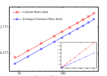
Figure 5: Computational complexity of the ${\bf J}$ and ${\bf K}_{\rm xc}$ matrix builds for cubic diamond at the RBLYP/6-21G* level of theory at the GOOD accuracy level.

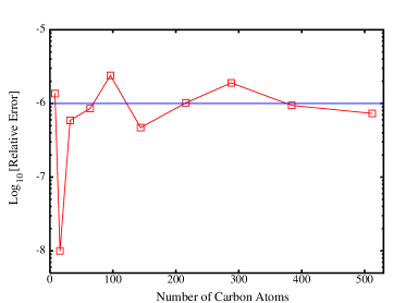
Figure 6: Relative error with system size for RBLYP/6-21G* diamond at the GOOD accuracy level.

Demonstrating linear scaling at the outset, Fig. 5 shows the CPU time for ${\bf J}$ and ${\bf K}_{\rm xc}$ builds with RBLYP/6-21G* diamond at its standard density. These timings correspond to a GOOD level of accuracy, targeting 6 digits in the total energy and corresponding to the values listed in Table4. Shown in Fig. 6 is the precision of the computed energies, obtained by performing a second set of calculations with all thresholds reduced by one order of magnitude. For these calculations, the largest source of error is the numerical integration performed by HiCu, as the QCTC thresholds are significantly more conservative.

VII Conclusions

We have extended linear scaling quantum chemical methods for computation of exchange-correlation and Coulomb matrices to periodic boundary conditions at the $\Gamma$-point. These methods have demonstrated an early onset of linear scaling and error control for diamond, allowing calculations up to 512 atoms at the RBLYP/6-21G* level of theory. In both cases, this early onset of linear scaling has been enabled by the use of modern data structures such as the $k$-d tree, together with reliable error estimates for the Gaussian extent. These algorithms have been parallelized Gan and Challacombe (2003); Gan et al. (2004a), demonstrating high efficiencies up to 128 processors, and have been used recently to determine the $T=0$K equation of state for pentaerythritol tetranitrate Gan et al. (2004b) at the RPBE/6-31G** level of theory and a GOOD accuracy level.

While this contribution has focused on demonstrating linear scaling for diamond, the methods presented here work for slabs and wires as well, using methods for computation of the two- and one-dimensional the $\cal M$ tensor outlined in Appendix A. Our experience has shown that, for the same number of atoms, these lower dimensional systems run much faster.

Appendix A Computation of the ${\cal M}$ Tensor

Following Nijboer and De Wette Nijboer and De Wette (1957, 1958), and later Challacombe, White and Head-Gordon Challacombe et al. (1997) (CWHG), we begin with the partition

$$\frac{1}{r^{l+1}}={\cal G}_{l}\left(\beta,r\right)+{\cal F}_{l}\left(\beta,r\right)$$ (26)

involving the functions

$${\cal G}_{l}\left(\beta,r\right)=\frac{\Gamma\left(l+\frac{1}{2},\beta^{2}r^{2}\right)}{\Gamma\left(l+\frac{1}{2}\right)\,r^{l+1}}$$ (27)

and

$${\cal F}_{l}\left(\beta,r\right)=\frac{\gamma\left(l+\frac{1}{2},\beta^{2}r^{2}\right)}{\Gamma\left(l+\frac{1}{2}\right)\,r^{l+1}}\,,$$ (28)

where $\Gamma$ is the gamma function, $\gamma$ is the incomplete gamma function Abramowitz and Stegun (1987) and $\beta$ is a parameter controlling the partition. With this separation of length scales, the lattice sum defining the multipole interaction tensor, ${\cal M}^{m}_{l}$, may be expressed as

$${\cal M}^{m}_{l} = \sum_{\mathbf{R}\in V_{\rm PFF}}\,M_{l}^{m}[\mathbf{R}]$$

$$= \sum_{\mathbf{R}\in V_{\rm PFF}}\widetilde{P}_{l}^{m}\left(\cos\theta_{\mathbf{R}}\right)e^{im\phi_{\mathbf{R}}}\,{\cal G}_{l}\left(\beta,\left|\mathbf{R}\right|\right)$$

$$+ \sum_{\mathbf{R}\in V_{\rm PFF}}\widetilde{P}_{l}^{m}\left(\cos\theta_{\mathbf{R}}\right)e^{im\phi_{\mathbf{R}}}\,{\cal F}_{l}\left(\beta,\left|\mathbf{R}\right|\right)\;.$$

Following CWHG, this expression can be further developed into real and reciprocal space terms:

$${\cal M}^{m}_{l} = \sum_{\mathbf{R}\in V_{\rm PFF}}\,\widetilde{P}_{l}^{m}\left(\cos\theta_{\mathbf{R}}\right)e^{im\phi_{\mathbf{R}}}\,{\cal G}_{l}\left(\beta,\left|\mathbf{R}\right|\right)$$

$$- \sum_{\mathbf{R}\in V_{\rm In}}\widetilde{P}_{l}^{m}\left(\cos\theta_{\mathbf{R}}\right)e^{im\phi_{\mathbf{R}}}{\cal F}_{l}\left(\beta,\left|\mathbf{R}\right|\right)$$

$$+ \frac{4\pi^{\frac{3}{2}}(\frac{i}{2})^{l}}{V_{\rm UC}\Gamma\left(l+\frac{1}{2}\right)}$$

$$\sum_{\mathbf{G}\neq\left\{\emptyset\right\}}\,\left|\mathbf{G}\right|^{l-2}e^{-\frac{\pi^{2}\left|\mathbf{G}\right|^{2}}{\beta^{2}}}\widetilde{P_{l}}^{m}\left(\cos\theta_{\mathbf{G}}\right)e^{im\phi_{\mathbf{G}}}\,,$$

where $\mathbf{G}$ are reciprocal lattice vectors. With an appropriate choice of $\beta\sim\sqrt{\pi}/\left(V_{\rm UC}\right)^{\frac{1}{3}}$, and summing terms from smallest to largest, the periodic multipole interaction tensor can be computed to high precision assuming an accurate representation of the incomplete gamma function. In previous work by CWHG, the upward recursion

$$\Gamma\left(m+1,\,x\right)=m\Gamma\left(m,\,x\right)+x^{m}e^{-x}$$ (31)

was used, which results in a loss of precision for large values of $x$ and $m$, demanding extended precision arithmetic and precluding on the fly computation. This problem is overcome by analytically summing the gamma function, collecting terms, and then rewriting it as

$$\Gamma\left(m+\frac{1}{2},\,x\right)=\Gamma\left(m+\frac{1}{2}\right)\qquad\qquad\qquad$$

$$\left\{{\rm erfc}\left(\sqrt{x}\right)+\sqrt{\frac{x}{\pi}}\sum_{n=0}^{m-1}(S_{n}\,x\,e^{-\frac{x}{n}})^{n}\right\}\,,$$ (32)

where the terms

$$S_{n}=\left(\frac{\Gamma\left(\frac{1}{2}\right)}{\Gamma\left(n+\frac{3}{2}\right)}\right)^{\frac{1}{{\rm max}(n,1)}}\,,$$ (33)

are simply pretabulated. This version of the gamma function is both easy to program and precise, even for large values of $x$ or $m$.

In one dimension, the ${\cal M}$ tensor can be computed analytically as

$${\cal M}^{m}_{l} = \frac{\widetilde{P}_{l}^{m}\left(\cos\theta_{0}\right)e^{im\phi_{0}}}{a_{0}^{l+1}}\sum_{n=n_{0}}^{\infty}\frac{1}{n^{l+1}}$$

$$+ \frac{\widetilde{P}_{l}^{m}\left(\cos\left(\theta_{0}+\frac{\pi}{2}\right)\right)e^{im\left(\phi_{0}+\pi\right)}}{a_{0}^{l+1}}\sum_{n=n_{0}}^{\infty}\frac{1}{n^{l+1}}$$

$$= Q_{l}^{m}\left[a_{0},\theta_{0},\phi_{0}\right]\left\{\zeta(l+1)-\sum_{n=1}^{n_{0}-1}\frac{1}{n^{l+1}}\right\}$$

where $a_{0}$, $\theta_{0}$ and $\phi_{0}$ are the initial box dimension and angles which are independent of the summation, and $\zeta$ is the Riemann zeta function Abramowitz and Stegun (1987).

In two dimensions, the Fourier integrals for the calculation of the ${\cal M}$ tensor become more complicated. Taking the limit as the box dimension in the non-periodic direction goes to infinity (the $z$ direction in the following), we obtain from Eq. LABEL:C4

$${\cal M}^{m}_{l} = \sum_{{\mathbf{R}}\in V_{\rm PFF}}\,\left(l-m\right)!\,P_{l}^{m}\left(\cos\theta_{\mathbf{R}}\right)e^{im\phi_{\mathbf{R}}}\,{\cal G}_{l}\left(\beta,\left|\mathbf{R}\right|\right)$$

$$- \sum_{{\mathbf{R}^{\prime}}\in V_{\rm In}}\,\left(l-m\right)!\,P_{l}^{m}\left(\cos\theta_{\mathbf{R}}\right)e^{im\phi_{\mathbf{R}}}{\cal F}_{l}\left(\beta,\left|\mathbf{R}\right|\right)$$

$$+ {\cal C}_{2}\sum_{\mathbf{G}\neq\left\{\emptyset\right\}}\,\int_{-\infty}^{\infty}\>dG_{z}\>\left|\mathbf{G}\right|^{l-2}e^{-\frac{\pi^{2}\left|\mathbf{G}\right|^{2}}{\beta^{2}}}\,$$

$$\qquad\qquad\qquad\qquad{\tilde{P}}_{l}^{m}\left(\cos\theta_{\mathbf{G}}\right)e^{im\phi_{\mathbf{G}}}\,,$$

where

$${\cal C}_{2}=\frac{4\pi^{\frac{3}{2}}(\frac{i}{2})^{l}}{A_{\rm UC}\Gamma\left(l+\frac{1}{2}\right)}$$ (36)

and $A_{\rm UC}$ is the area of the cell along the non-periodic direction. In practice, we carry out numerical evaluation of this integral.

References

- Honda et al. (1991) M. Honda, K. Sato, and S. Obara, J. Chem. Phys. 94, 3790 (1991).
- Helgaker and Taylor (1992) T. Helgaker and P. R. Taylor, Theo. Chim. Acta 83, 177 (1992).
- Stephens et al. (1994) P. J. Stephens, F. J. Devlin, C. F. Chabalowski, and M. J. Frisch, J. Phys. Chem. 98, 11623 (1994).
- Helgaker et al. (2001) T. Helgaker, H. Jensen, P. Jorgensen, J. Olsen, K. Ruud, H. Ågren, A. Auer, K. Bak, V. Bakken, O. Christiansen, S. Coriani, P. Dahle, et al., Dalton, a molecular electronic structure program, Release 1.2 (2001), URL http://www.kjemi.uio.no/software/dalton/dalton.html.
- Laerdahl et al. (1997) J. K. Laerdahl, T. Saue, and K. Faegri, Theor. Chem. Acc. 97(1-4), 177 (1997).
- Grant and Quiney (2000) I. P. Grant and H. M. Quiney, Int. J. Quant. Chem. 80(3), 283 (2000).
- Yanai et al. (2001) T. Yanai, H. Iikura, T. Nakajima, Y. Ishikawa, and K. Hirao, J. Chem. Phys 115(18), 8267 (2001).
- Gill et al. (1992) P. M. Gill, B. J. Johnson, J. A. Pople, and M. J. Frisch, Int. J. Quant. Chem. S26, 319 (1992).
- Becke (1993) A. D. Becke, J. Chem. Phys. 98, 1372 (1993).
- Barone et al. (1996) V. Barone, C. Adamo, and F. Mele, Chem. Phys. Lett. 249, 290 (1996).
- Adamo et al. (1999) C. Adamo, M. Cossi, and V. Barone, Theochem 493, 145 (1999).
- Saunders et al. (1998) V. Saunders, R. Dovesi, C. Roetti, M. Causà, N. Harrison, R. Orlando, and C. M. Zicovich-Wilson, CRYSTAL98, http://www.chimifm.unito.it/teorica/crystal/ (1998).
- Bredow and Gerson (2000) T. Bredow and A. R. Gerson, Phys. Rev. B 61(8), 5194 (2000).
- Muscat et al. (2001) J. Muscat, A. Wander, and N. M. Harrison, Chem. Phys. Lett. 342, 397 (2001).
- Baranek et al. (2001) P. Baranek, A. Lichanot, R. Orlando, and R. Dovesi, Chem. Phys. Lett. 340, 362 (2001).
- Wander and Harrison (2001) A. Wander and N. M. Harrison, J. Chem. Phys. 105(26), 6191 (2001).
- Challacombe and Schwegler (1997) M. Challacombe and E. Schwegler, J. Chem. Phys. 106, 5526 (1997).
- Challacombe (2000) M. Challacombe, J. Chem. Phys. 113, 10037 (2000).
- Niklasson (2002) A. M. N. Niklasson, Phys. Rev. B 66, 155115 (2002).
- Niklasson et al. (2003) A. M. N. Niklasson, C. J. Tymczak, and M. Challacombe, J. Chem. Phys. 118(19), 8611 (2003).
- Tymczak et al. (2004) C. J. Tymczak, V. Weber, E. Schwegler, and M. Challacombe, Linear scaling computation of the Fock matrix. VIII. Periodic boundaries for exact exchange at the -point (2004), submitted to Phys. Rev. B.
- Niklasson and Challacombe (2004) A. M. N. Niklasson and M. Challacombe, Phys. Rev. Lett. 92, 193001 (2004).
- Weber et al. (2004) V. Weber, A. M. N. Niklasson, and M. Challacombe, Phys. Rev. Lett. 92, 193002 (2004).
- Nijboer and De Wette (1957) B. R. A. Nijboer and F. W. De Wette, Physica 23, 309 (1957).
- Nijboer and De Wette (1958) B. R. A. Nijboer and F. W. De Wette, Physica 24(6), 422 (1958).
- Challacombe et al. (2001) M. Challacombe, E. Schwegler, C. J. Tymczak, C. K. Gan, K. Nemeth, V. Weber, A. M. N. Niklasson, and G. Henkelman, MondoSCF v1.09, A program suite for massively parallel, linear scaling SCF theory and ab initio molecular dynamics. (2001), URL http://www.t12.lanl.gov/home/mchalla/, Los Alamos National Laboratory (LA-CC 01-2), Copyright University of California.
- Towler (2000) M. Towler, An introductory guide to Gaussian basis sets in solid-state electronic structure calculations (2000), notes for Summer School, Torino.
- Dovesi et al. (2003) R. Dovesi, V. Saunders, C. Roetti, M. Causa, N. Harrison, R. Orlando, and C. Zicovich-Wilson, CRYSTAL98 Basis Sets, http://www.crystal.unito.it/Basis_Sets/ptable.html (2003).
- Towler (1998) M. Towler, CRYSTAL98 Basis Sets, http://www.tcm.phy.cam.ac.uk/~mdt26/crystal.html (1998).
- Grüneich and Hess (1998) A. Grüneich and B. A. Hess, Theor. Chem. Acc. 100(1-4), 253 (1998).
- Gomez (1999) M. Gomez, Simple Intersection Tests for Games (1999), URL http://www.gamasutra.com/.
- Tymczak and Challacombe (2003) C. J. Tymczak and M. Challacombe (2003), in preparation.
- Challacombe et al. (1997) M. Challacombe, C. White, and M. Head-Gordon, J. Chem. Phys. 107, 10131 (1997).
- Ahmadi and Almlöf (1995) G. R. Ahmadi and J. Almlöf, Chem. Phys. Lett. 246, 364 (1995).
- McMurchie and Davidson (1978) L. E. McMurchie and E. R. Davidson, J. Comp. Phys. 26, 218 (1978).
- Hille (1926) E. Hille, Ann. Math. 27, 427 (1926).
- Redlack and Grindlay (1972) A. Redlack and J. Grindlay, Can. J. Phys. 50, 2815 (1972).
- Becke (1988a) A. D. Becke, J. Chem. Phys. 88, 2547 (1988a).
- Pople et al. (1992) J. A. Pople, P. M. W. Gill, and B. G. Johnson, Chem. Phys. Lett. 199(6), 557 (1992).
- Gan and Challacombe (2003) C. K. Gan and M. Challacombe, J. Chem. Phys. 118, 9128 (2003).
- Glassner (1990) A. S. Glassner, ed., Graphics Gems (Academic Press, 1990).
- The Portland Group (2002) The Portland Group, pgf90 v4.2 (2002), URL http://www.pgroup.com/.
- Redhat (2004) Redhat, Redhat v9.0, http://www.redhat.com/ (2004).
- Prencipe et al. (1995) M. Prencipe, A. Zupan, R. Dovesi, E. Apra, and V. R. Saunders, Phys. Rev. B 51(6), 3391 (1995).
- Harrison and Saunders (1992) N. M. Harrison and V. R. Saunders, J. Phys. 4(15), 3873 (1992).
- Lee et al. (1988) C. T. Lee, W. T. Yang, and R. G. Parr, Phys. Rev. B 37(2), 785 (1988).
- Becke (1988b) A. D. Becke, Phys. Rev. A 38(6), 3098 (1988b).
- Causa et al. (1986) M. Causa, R. Dovesi, C. Pisani, and C. Roetti, Phys. Rev. B 33(2), 1308 (1986).
- PBC (2004) Periodic coordinates used in MondoSCF validation (2004), URL http://www.t12.lanl.gov/~mchalla/.
- Catti et al. (1993) M. Catti, A. Pavese, R. Dovesi, and V. R. Saunders, Phys. Rev. B 47(15), 9189 (1993).
- Gan et al. (2004a) C. K. Gan, C. J. Tymczak, and M. Challacombe, Linear Scaling Computation of the Fock Matrix. IX. Parallel Computation of the Coulomb Matrix (2004a), submitted to J. Chem. Phys.
- Gan et al. (2004b) C. K. Gan, T. D. Sewell, and M. Challacombe, Phys. Rev. B 69, 035116 (2004b).
- Abramowitz and Stegun (1987) M. Abramowitz and I. A. Stegun, eds., Handbook of Mathematical Functions (Dover Publications Inc., New York, 1987), ninth ed.