Hyperfine interaction in a quantum dot: Non-Markovian electron spin dynamics

Abstract

We have performed a systematic calculation for the non-Markovian dynamics of a localized electron spin interacting with an environment of nuclear spins via the Fermi contact hyperfine interaction. This work applies to an electron in the $s$-type orbital ground state of a quantum dot or bound to a donor impurity, and is valid for arbitrary polarization $p$ of the nuclear spin system, and arbitrary nuclear spin $I$ in high magnetic fields. In the limit of $p=1$ and $I=\frac{1}{2}$, the Born approximation of our perturbative theory recovers the exact electron spin dynamics. We have found the form of the generalized master equation (GME) for the longitudinal and transverse components of the electron spin to all orders in the electron spin–nuclear spin flip-flop terms. Our perturbative expansion is regular, unlike standard time-dependent perturbation theory, and can be carried-out to higher orders. We show this explicitly with a fourth-order calculation of the longitudinal spin dynamics. In zero magnetic field, the fraction of the electron spin that decays is bounded by the smallness parameter $\delta=1/p^{2}N$, where $N$ is the number of nuclear spins within the extent of the electron wave function. However, the form of the decay can only be determined in a high magnetic field, much larger than the maximum Overhauser field. In general the electron spin shows rich dynamics, described by a sum of contributions with non-exponential decay, exponential decay, and undamped oscillations. There is an abrupt crossover in the electron spin asymptotics at a critical dimensionality and shape of the electron envelope wave function. We propose a scheme that could be used to measure the non-Markovian dynamics using a standard spin-echo technique, even when the fraction that undergoes non-Markovian dynamics is small.

I Introduction

Prospects for the development of new spintronic devices,Wolf et al. (2001) and the controlled manipulation of electron or nuclear spins for quantum information processingAwschalom et al. (2002) have sparked substantial research efforts in recent years. One of the major obstacles to achieving these goals is decoherence due to the influence of an uncontrollable environment. For quantum computing tasks, the strict requirements for error correctionPreskill (1998) put strong limits on the degree of decoherence allowed in such devices. From this point of view, single-electron semiconductor quantum dots represent good candidates for spin-based information processing since they show particularly long longitudinal relaxation times, $T_{1}=1\,\mathrm{ms}$.Kouwenhoven et al. In GaAs quantum wells, the transverse dephasing time $T_{2}^{*}$ for an ensemble of electron spins, which typically provides a lower bound for the intrinsic decoherence time $T_{2}$ of an isolated spin, has been measured to be in excess of $100\,\mathrm{ns}$.Kikkawa and Awschalom (1998)

Possible sources of decoherence for a single electron spin confined to a quantum dot are spin-orbit coupling and the contact hyperfine interaction with the surrounding nuclear spins.Burkard et al. (1999) The relaxation rate due to spin-orbit coupling $\frac{1}{T_{1}}$ is suppressed for localized electrons at low temperaturesKhaetskii and Nazarov (2000, 2001) and recent work has shown that $T_{2}$, due to spin-orbit coupling, can be as long as $T_{1}$ under realistic conditions.Golovach et al. (2003) However, since spin-carrying isotopes are common in the semiconductor industry, the contact hyperfine interaction (in contrast to the spin-orbit interaction) is likely an unavoidable source of decoherence, which does not vanish with decreasing temperature or carefully chosen quantum dot geometry.Schliemann et al. (2003)

In the last few years, a great deal of effort has been focused on a theoretical description of interesting effects arising from the contact hyperfine interaction for a localized electron.Burkard et al. (1999); Khaetskii et al. (2002a, b); Schliemann et al. (2002); Lyanda-Geller et al. (2002); Taylor et al. (2003a, b); Imamoglu et al. (2003); Semenov and Kim (2004); Erlingsson et al. (2001); Erlingsson and Nazarov (2002); de Sousa and S. Das Sarma (2003a, b); Semenov and Kim (2003); Merkulov et al. (2002); Saykin et al. (2002) The predicted effects include a dramatic variation of $T_{1}$ with gate voltage in a quantum dot near the Coulomb blockade peaks or valleys,Lyanda-Geller et al. (2002) all-optical polarization of the nuclear spins,Imamoglu et al. (2003) use of the nuclear spin system as a quantum memory,Taylor et al. (2003a, b) and several potential spin relaxation and decoherence mechanisms.Khaetskii et al. (2002a); Erlingsson et al. (2001); Erlingsson and Nazarov (2002); Semenov and Kim (2004); de Sousa and S. Das Sarma (2003a) This theoretical work is spurred-on by intriguing experiments that show localized electrical detection of spin resonance phenomena,Dobers et al. (1988) nuclear spin polarization near quantum point contacts,Wald et al. (1994) gate-controlled transfer of polarization between electrons and nuclei,Smet et al. (2002) nuclear spin polarization and manipulation due to optical pumping in GaAs quantum wells,Salis et al. (2001) and voltage-controlled nuclear spin polarization in a field-effect transistor.Epstein et al. (2003) In addition, recent experiments have shown hyperfine induced oscillations in transport current through a double quantum dot,Ono and Tarucha (2003) and long $T_{2}$ times for electrons trapped at shallow donor impurities in isotopically purified ²⁸Si:P.Tyryshkin et al. (2003) Our system of interest in this paper is an electron confined to a single GaAs quantum dot, but this work applies quite generally to other systems, such as electrons trapped at shallow donor impurities in Si:P.Schliemann et al. (2003)

In this paper, we investigate electron spin dynamics at times shorter than the nuclear dipole-dipole correlation time $\tau_{\mathrm{dd}}$ ($\tau_{\mathrm{dd}}\approx 10^{-4}\,\mathrm{s}$ in GaAs is given directly by the inverse width of the nuclear magnetic resonance (NMR) linePaget et al. (1977)). At these time scales, the relevant Hamiltonian for a description of the electron and nuclear spin dynamics is that for the Fermi contact hyperfine interaction (see Eq. (1), below). Dynamics under the action of this Hamiltonian may be of fundamental interest, since in zero magnetic field, Eq. (1) corresponds to the well-known integrable Gaudin magnet, which is soluble via Bethe ansatz.Gaudin (1976); Schliemann et al. (2003) Though the Hamiltonian appears simple, a detailed microscopic description for the dynamics of a spin coupled to a spin environment remains an open question.Dobrovitski et al. (2003); Zurek et al. (2003) A degree of success has been achieved some time ago in bulk systems through the development of phenomenological models.Klauder and Anderson (1962) These models invoke certain approximations, namely, assumptions of Markovian dynamics and ensemble averaging. Care should therefore be taken in applying the same models to the problem of single-spin decoherence for an electron spin strongly coupled to a nuclear spin environment, where they may not apply.Khaetskii et al. (2002a, b)

For nuclear spin $I=\frac{1}{2}$, an exact solution for the electron spin dynamics has been found in the special case of a fully polarized initial state of the nuclear spin system.Khaetskii et al. (2002a, b) This solution shows that the electron spin only decays by a fraction $\propto\frac{1}{N}$ of its initial value, where $N$ is the number of nuclear spins within the extent of the electron wave function. The decaying fraction was shown to have a non-exponential tail for long times, which suggests non-Markovian (history dependent) behavior. For an initial nuclear spin configuration that is not fully polarized, no exact solution is available and standard time-dependent perturbation theory fails.Khaetskii et al. (2002a) Subsequent exact diagonalization studies on small spin systemsSchliemann et al. (2002) have shown that the electron spin dynamics are highly dependent on the type of initial nuclear spin configuration, and the dynamics of a randomly correlated initial nuclear spin configuration are reproduced by an ensemble average over direct-product initial states. The unusual (non-exponential) form of decay, and the fraction of the electron spin that undergoes decay may be of interest in quantum error correction (QEC) since QEC schemes typically assume exponential decay to zero.

In this paper we formulate a systematic perturbative theory of electron spin dynamics under the action of the Fermi contact hyperfine interaction. This theory is valid for arbitrary nuclear spin polarization and arbitrary nuclear spin $I$ in high magnetic fields. For nuclear spin $I=\frac{1}{2}$ and a fully polarized nuclear spin system, we recover the exact solution for the electron spin dynamics within the Born approximation of our perturbative theory. Our approach follows a method recently applied to the spin-boson model.Loss and DiVincenzo (2003) This method does not suffer from unbounded secular terms that occur in standard perturbation theoryKhaetskii et al. (2002a) and does not involve Markovian approximations.

This paper is organized as follows. In Section II we review the model Hamiltonian and address the question of realistic initial conditions. In Section III we derive the form of the exact generalized master equation (GME) for the electron spin dynamics. In Section IV we consider the leading-order electron spin dynamics in high magnetic fields. In Section V we proceed to calculate the complete non-Markovian dynamics within the Born approximation. We describe a procedure that could be used to measure the non-Markovian dynamics in Section VI. In Section VII we show that our method can be extended to higher orders without the problems of standard perturbation theory by explicitly calculating the corrections to the longitudinal spin self-energy at fourth order in the nuclear spin–electron spin flip-flop terms. We conclude in Section VIII with a summary of the results. Technical details are deferred to Appendices A–E.

II Model

II.1 Hamiltonian

We consider a localized electron spin interacting with $N_{\mathrm{tot}}$ nuclear spins via the Fermi contact hyperfine interaction. The Hamiltonian for this system is

$$\mathcal{H}=bS_{z}+\epsilon_{nz}I_{z}+\mathbf{h}\cdot\mathbf{S},$$ (1)

where $\mathbf{S}=\left(S_{x},S_{y},S_{z}\right)$ is the electron spin operator. $b=g^{*}\mu_{B}B_{z}\,(\epsilon_{nz}=g_{I}\mu_{N}B_{z})$ is the electron (nuclear) Zeeman splitting in a magnetic field $B_{z}$, with effective g-factor $g^{*}$ ($g_{I}$) for the electron (nuclei) and Bohr (nuclear) magneton $\mu_{B}$ ($\mu_{N}$). Further, $\mathbf{h}=\left(h_{x},h_{y},h_{z}\right)=\sum_{k=0}^{N_{\mathrm{tot}}-1}A_{k}\mathbf{I}_{k}$ gives the (quantum) field generated by an environment of nuclear spins. $\mathbf{I}_{k}=\left(I_{k}^{x},I_{k}^{y},I_{k}^{z}\right)$ is the nuclear spin operator at lattice site $k$ and $A_{k}$ is the associated hyperfine coupling constant. $I_{z}=\sum_{k}I_{k}^{z}$ is the total $z$-component of nuclear spin.

The nuclear Zeeman term can be formally eliminated from the Hamiltonian $\mathcal{H}$ (Eq. (1)) by transforming to a rotating reference frame. The $z$-component of total angular momentum is $J_{z}=S_{z}+I_{z}$. Adding and subtracting $\epsilon_{nz}J_{z}$ gives $\mathcal{H}=\mathcal{H}^{\prime}+\epsilon_{nz}J_{z}$. The Hamiltonian in the rotating frame, $\mathcal{H}^{\prime}$, is then

$$\mathcal{H}^{\prime} = \mathcal{H}_{0}^{\prime}+\mathcal{H}_{V}^{\prime},$$ (2)

$$\mathcal{H}_{0}^{\prime} = b^{\prime}S_{z}+h_{z}S_{z},$$ (3)

$$\mathcal{H}_{V}^{\prime} = \frac{1}{2}\left(h_{+}S_{-}+h_{-}S_{+}\right),$$ (4)

where $b^{\prime}=b-\epsilon_{nz}$ and we have introduced $h_{\pm}=h_{x}\pm ih_{y}$. The usual Heisenberg-picture operators in the rotating frame are $S_{X}^{\prime}(t)=e^{i\mathcal{H}^{\prime}t}S_{X}e^{-i\mathcal{H}^{\prime}t},\,X=z,+,\,S_{\pm}=S_{x}\pm iS_{y}$. Noting that $\left[J_{z},\mathcal{H}\right]=0$, we find they are related to the operators $S_{X}(t)=e^{i\mathcal{H}t}S_{X}e^{-i\mathcal{H}t}$ in the rest frame by

$$S_{z}^{\prime}(t) = S_{z}(t)$$ (5)

$$S_{+}^{\prime}(t) = e^{-i\epsilon_{nz}t}S_{+}(t).$$ (6)

In the following, $\left\langle S_{z}^{\prime}\right\rangle_{t}$ and $\left\langle S_{+}^{\prime}\right\rangle_{t}$ will be evaluated in the rotating frame, but we omit primes on all expectation values.

The hyperfine coupling constants $A_{k}$ are given bySchliemann et al. (2003)

$$A_{k}=Av_{0}|\psi(\mathbf{r}_{k})|^{2}.$$ (7)

Here, $v_{0}$ is the volume of a crystal unit cell containing one nuclear spin, $\psi(\mathbf{r})$ is the electron envelope wave function, and $A$ is the strength of the hyperfine coupling. In GaAs, all naturally occurring isotopes carry spin $I=\frac{3}{2}$. In bulk GaAs, $A$ has been estimatedPaget et al. (1977) to be $A=90\,\mu eV$ $\left(\frac{A}{|g^{*}|\mu_{B}}=3.5\,\mathrm{T}\right)$. This estimate is based on an average over the hyperfine coupling constants for the three nuclear isotopes $\mathrm{{}^{69}Ga}$, $\mathrm{{}^{71}Ga}$, and $\mathrm{{}^{75}As}$, weighted by their relative abundances. Natural silicon contains 4.7% ${}^{29}\mathrm{Si}$, which carries $I=\frac{1}{2}$, and 95% ${}^{28}\mathrm{Si}$, with $I=0$. An electron bound to a phosphorus donor impurity in natural Si:P interacts with $N\approx 10^{2}$ surrounding $\mathrm{{}^{29}Si}$ nuclear spins, in which case the hyperfine coupling constant is on the order of $A\approx 0.1\,\mu eV$.Schliemann et al. (2003) We consider a localized electron in its orbital ground state, described by an isotropic envelope wave function of the form

$$\psi(r_{k})=\psi(0)\exp\left[-\frac{1}{2}\left(\frac{r_{k}}{l_{0}}\right)^{m}\right].$$ (8)

When $m=2$, $\psi(r)$ is a Gaussian with Bohr radius $l_{0}$, and for $m=1$, $\psi(r)$ corresponds to a hydrogen-like $s$-state with Bohr radius $a_{0}=2l_{0}$. $N_{\mathrm{tot}}$ nuclear spins are in the system, but the effective number $N$ of spins interacting appreciably with the electron is smaller (see Fig. 1). $N$ is defined as the number of nuclear spins within radius $l_{0}$ of the origin and the integer index $k$ gives the number of spins within radius $r_{k}$. In $d$ dimensions, $\left(\frac{r_{k}}{l_{0}}\right)^{d}=\frac{k}{N}$. It is convenient to work in energy units such that $\frac{A_{0}}{2}=1$, where $A_{0}$ is the coupling constant at the origin $(r_{0}=0)$. In these units $A_{k}$ takes the simple form

$$A_{k}=2\exp\left[-\left(\frac{k}{N}\right)^{\frac{m}{d}}\right].$$ (9)

Figure 1: Schematic of the square modulus of the electron envelope wave function $\left|\psi(r)\right|^{2}$ and nuclear spins (arrows). $k$ is the nuclear site index, $N$ is the number of nuclear spins within radius $r=l_{0}$, and $N_{\mathrm{tot}}$ is the total number of nuclear spins in the system.

II.2 Initial conditions

II.2.1 Sudden approximation

The electron spin and nuclear system are decoupled for times $t<0$, and prepared independently in states described by the density operators $\rho_{S}(0)$ and $\rho_{I}(0)$, respectively. At $t=0$, the electron and nuclear spin system are brought into contact “instantaneously”, i.e., the electron spin and nuclear system are brought into contact over a switching time scale $\tau_{\mathrm{sw}}$, which is sufficiently small–see Eq. (11), below. The state of the entire system, described by the total density operator $\rho(t)$ is then continuous at $t=0$, and is given by

$$\rho(0^{-})=\rho(0^{+})=\rho_{S}(0)\otimes\rho_{I}(0).$$ (10)

The evolution of the density operator $\rho(t)$ for $t\geq 0$ is governed by the Hamiltonian $\mathcal{H}^{\prime}$ for an electron spin coupled to an environment of nuclear spins. Since the largest energy scale in this problem is given by $\left|b^{\prime}+A\right|$, in general the condition

$$\tau_{\mathrm{sw}}\ll\frac{2\pi\hbar}{\left|b^{\prime}+A\right|}$$ (11)

should be satisfied for the sudden approximation (Eq. (10)) to be valid. In bulk GaAs, $\frac{2\pi\hbar}{A}\simeq 50\,\mathrm{ps}$ and for an electron bound to a phosphorus donor in natural silicon, $\frac{2\pi\hbar}{A}\simeq 10\,\mathrm{ns}$.

II.2.2 Dependence on the nuclear state: zeroth order dynamics

Evolution of the electron spin for different initial nuclear configurations has been addressed previously.Khaetskii et al. (2002b); Schliemann et al. (2002) In Ref. Schliemann et al., 2002 it was found, through numerical study, that the dynamics of the electron spin were highly dependent on the initial state of the nuclear system. The goal of this section is to shed more light on the role of the initial nuclear configuration by evaluating the much simpler zeroth order dynamics, i.e., the electron spin evolution is evaluated under $\mathcal{H}^{\prime}=\mathcal{H}_{0}^{\prime}$ alone, neglecting the flip-flop terms $\mathcal{H}_{V}^{\prime}$.

Since $\left[\mathcal{H}_{0}^{\prime},S_{z}\right]=0$, $\left\langle S_{z}\right\rangle_{t}$ is constant. However, $\left[\mathcal{H}_{0}^{\prime},S_{\pm}\right]\neq 0$, so the transverse components, $\left\langle S_{+}\right\rangle_{t}=\left\langle S_{x}\right\rangle_{t}+i\left\langle S_{y}\right\rangle_{t}$, will have a nontrivial time dependence. We evaluate the expectation value $\left\langle S_{+}\right\rangle_{t}=\mathrm{Tr}\left\{e^{-i\mathcal{H}_{0}^{\prime}t}S_{+}e^{i\mathcal{H}_{0}^{\prime}t}\rho(0)\right\}$ (setting $\hbar=1$), with the initial state given in Eq. (10). After performing a partial trace over the electron spin Hilbert space, we obtain an expression in terms of the initial nuclear spin state:

$$\left\langle S_{+}\right\rangle_{t}=\left\langle S_{+}\right\rangle_{0}\mathrm{Tr}_{I}\left\{e^{i(b^{\prime}+h_{z})t}\rho_{I}(0)\right\},$$ (12)

where $\mathrm{Tr}_{I}$ is a partial trace over the nuclear spin space alone. For simplicity, here we consider $I=\frac{1}{2}$, and the coupling constants are taken to be uniform. After enforcing the normalization $\sum_{k}A_{k}=2N$ in units where $\frac{A_{0}}{2}=\frac{A}{2N}=1$, the hyperfine coupling constants are

$$A_{k}=\left\{\begin{array}[]{l}2,\,\,\,k=0,1\cdots N-1\\ 0,\,\,\,k\geq N\end{array}\right..$$ (13)

The zeroth-order electron spin dynamics can now be evaluated exactly for three types of initial nuclear spin configuration:

$$\rho_{I}^{(1)}(0) = \left|\psi_{I}(0)\right\rangle\left\langle\psi_{I}(0)\right|$$ (14)

$$\rho_{I}^{(2)}(0) = \sum_{N_{\uparrow}=0}^{N}P(N_{\uparrow};N,f_{\uparrow})\left|N_{\uparrow}\right\rangle\left\langle N_{\uparrow}\right|$$ (15)

$$\rho_{I}^{(3)}(0) = \left|n\right\rangle\left\langle n\right|.$$ (16)

$\rho_{I}^{(1)}$ is a pure state, where $\left|\psi_{I}(0)\right\rangle=\prod_{k=0}^{N}\left(\sqrt{f_{\uparrow}}\left|\uparrow_{k}\right\rangle+e^{i\phi_{k}}\sqrt{1-f_{\uparrow}}\left|\downarrow_{k}\right\rangle\right)$ is chosen to render the z-component of nuclear spin translationally invariant: $\left\langle\psi_{I}(0)\right|I_{k}^{z}\left|\psi_{I}(0)\right\rangle=\frac{1}{2}(2f_{\uparrow}-1)=\frac{p}{2}$ , and $p=2f_{\uparrow}-1$ is the polarization of the nuclear spin system. $\phi_{k}$ is an arbitrary site-dependent phase factor. $P(x;n,f)=\left(\begin{array}[]{c}n\\ x\end{array}\right)f^{x}(1-f)^{n-x}$ is a binomial distribution, and $\left|N_{\uparrow}\right\rangle$ is a product state of the form $\left|\uparrow\uparrow\downarrow\cdots\right\rangle$ with $N_{\uparrow}$ spins up and $N-N_{\uparrow}$ spins down. $\rho_{I}^{(2)}(0)$ then corresponds to a mixed state; this is an ensemble of product states where the $N$ spins in each product state are selected from a bath of polarization $p=2f_{\uparrow}-1$. $\rho_{I}^{(3)}$, like $\rho_{I}^{(1)}$, is a pure state, but for this state $\left|n\right\rangle$ is chosen to be an eigenstate of $h_{z}$ with eigenvalue $pN$ (corresponding to a nuclear system with polarization $p$): $h_{z}\left|n\right\rangle=pN\left|n\right\rangle$. We insert the initial nuclear spin states $\rho_{I}^{(i)}(0)$ into (12) to obtain the associated time evolution $\left\langle S_{+}\right\rangle_{t}^{(i)}$:

$$\left\langle S_{+}\right\rangle_{t}^{(1,2)} =\left\langle S_{+}\right\rangle_{0} \sum_{N_{\uparrow}=0}^{N}P(N_{\uparrow};N,f_{\uparrow})e^{i(b^{\prime}+M(N_{\uparrow}))t},\,\,$$ (17)

$$\left\langle S_{+}\right\rangle_{t}^{(3)} = \left\langle S_{+}\right\rangle_{0}\mathrm{e}^{i(b^{\prime}+pN)t}.$$ (18)

$M(N_{\uparrow})=2N_{\uparrow}-N$ is the nuclear magnetization on a dot with $N_{\uparrow}$ nuclear spins up.

The similarity in dynamics between randomly correlated (entangled) pure states and mixed states has been demonstrated for evolution under the full Hamiltonian $(\mathcal{H}^{\prime}=\mathcal{H}_{0}^{\prime}+\mathcal{H}_{V}^{\prime})$ via exact diagonalizations of small ($N_{\mathrm{tot}}\lesssim 19$) spin systems.Schliemann et al. (2002) Here, the zeroth order electron spin dynamics are identical for the pure state $\rho_{I}^{(1)}(0)$ and the mixed state $\rho_{I}^{(2)}(0)$ even when the initial pure state $\left|\psi_{I}(0)\right\rangle$ is a direct product. Direct application of the central limit theorem gives a Gaussian decay for large $N$:

$$\left\langle S_{+}\right\rangle_{t}^{(1,2)}\approx\left\langle S_{+}\right\rangle_{0}e^{-\frac{t^{2}}{2t_{\mathrm{c}}^{2}}+i(b^{\prime}+pN)t},\,t_{\mathrm{c}}=\frac{1}{\sqrt{N(1-p^{2})}}.$$ (19)

Returning to dimension-full units (c.f. Table 1 below), the time scale for this decay is given by $\tau_{\mathrm{c}}=\frac{2N\hbar}{A}t_{\mathrm{c}}\approx 5\,\mathrm{ns}$ for a GaAs quantum dot with $p^{2}\ll 1$ containing $N=10^{5}$ nuclei and $\tau_{c}\approx 100\,\mathrm{ns}$ for an electron trapped at a shallow donor impurity in $\mathrm{Si:P}$, with $N=10^{2}$. For an ensemble of nuclear spin states, Gaussian decay with the time scale $\tau_{c}$ has been found previously.Khaetskii et al. (2002a, b); Merkulov et al. (2002) Gaussian decay for a Hamiltonian with an Ising coupling of electron and nuclear spins has been demonstratedZurek et al. (2003) for a more general class of $pure$ initial states and for coupling constants $A_{k}$ that may vary from site-to-site.

For the initial states $\rho_{I}^{(1,2)}(0)$, precise control over the nuclear spin polarization between measurements or a spin-echo technique would be needed to reduce or eliminate the rapid decay described by (19). However, the quantum superposition of $h_{z}$ eigenstates can be removed, in principle, from the pure state $\rho_{I}^{(1)}(0)$ by performing a strong (von Neumann) measurement on the nuclear Overhauser field $pN$. After the nuclear system is prepared in an $h_{z}$-eigenstate, to zeroth order the electron spin dynamics will be given by $\left\langle S_{+}\right\rangle_{t}^{(3)}$, i.e., a simple precession about the z-axis with no decay.

When higher-order corrections are taken into account, and the coupling constants $A_{k}$ are allowed to vary from site-to-site, even an initial $h_{z}$-eigenstate can lead to decay of the electron spin. This has been shownKhaetskii et al. (2002a, b) in an exact solution for the specific case of a fully-polarized system of nuclear spins-$\frac{1}{2}$ and by exact diagonalization on small systems.Schliemann et al. (2002) The goal of the present work is to perform an analytical calculation with a larger range of validity (a large system of nuclear spins with arbitrary polarization and arbitrary nuclear spin $I$ in a sufficiently strong magnetic field) that recovers previous exact results in the relevant limiting cases. In the rest of this paper, the effect of higher- (beyond zeroth-) order corrections will be considered for a nuclear spin system prepared in an arbitrary $h_{z}$ eigenstate: $\rho_{I}(0)=\rho_{I}^{(3)}(0)$, as given in Eq. (16). Specifically, the initial state of the nuclear system $\left|n\right\rangle$ can be written as an arbitrary linear combination of $g_{n}$ degenerate product states:

$$\left|n\right\rangle=\sum_{j=1}^{g_{n}}\alpha_{j}\left|n_{j}\right\rangle,\,\,\,\,\,\left|n_{j}\right\rangle=\bigotimes_{i=0}^{N_{\mathrm{tot}}-1}\left|I,m_{i}^{j}\right\rangle$$ (20)

where $\left|I,m_{i}\right\rangle$ is an eigenstate of the operator $I_{i}^{z}$ with eigenvalue $m_{i}$ and $h_{z}\left|n_{j}\right\rangle=\left[h_{z}\right]_{nn}\left|n_{j}\right\rangle$ for all $j$, where we write the matrix elements of any operator $\mathcal{O}$ as $\left\langle i\right|\mathcal{O}\left|j\right\rangle=\left[\mathcal{O}\right]_{ij}$.

III Generalized master equation

To evaluate the dynamics of the reduced (electron spin) density operator, we introduce a projection superoperator $P$, defined by its action on an arbitrary operator $\mathcal{O}$: $P\mathcal{O}=\rho_{I}(0)\mathrm{Tr}_{I}\mathcal{O}$. $P$ is chosen to preserve all electron spin expectation values: $\left\langle S_{\beta}\right\rangle_{t}=\mathrm{Tr}S_{\beta}\rho(t)=\mathrm{Tr}S_{\beta}P\rho(t),\,\beta=x,y,z$, and satisfies $P^{2}=P$. For factorized initial conditions (Eq. (10)), $P\rho(0)=\rho(0)$, which is a sufficient condition to rewrite the von Neumann equation $\dot{\rho}(t)=-i\left[\mathcal{H}^{\prime},\rho(t)\right]$ in the form of the exact Nakajima-Zwanzig generalized master equation (GME)Fick and Sauermann (1990):

$$P\dot{\rho}(t) = -iPLP\rho(t)-i\int_{0}^{t}dt^{\prime}\Sigma(t-t^{\prime})\rho(t^{\prime}),$$ (21)

$$\Sigma(t) = -iPLQe^{-iLQt}QLP,$$ (22)

where $\Sigma(t)$ is the self-energy superoperator and $Q=\mathbf{1}-P$ is the complement of $P$ ($\mathbf{1}$ is the identity superoperator). $L=L_{0}+L_{V}$ is the full Liouvillian, where $L_{\alpha}$ $(\alpha=V,0)$ is defined by $L_{\alpha}\mathcal{O}=\left[\mathcal{H}_{\alpha}^{\prime},\mathcal{O}\right]$. When the initial nuclear state is of the form $\rho_{I}(0)=\left|n\right\rangle\left\langle n\right|$, where $\left|n\right\rangle$ is an arbitrary eigenstate of $h_{z}$, as in Eq. (20), $P$ obeys the useful identities

$$PL_{V}P = 0,$$ (23)

$$PL_{0}P = L_{0}P.$$ (24)

We apply Eqs. (23) and (24), and perform a trace on (21) over the nuclear spins to obtain

$$\dot{\rho}_{S}(t) = -iL_{0}^{n}\rho_{S}(t)-i\int_{0}^{t}dt^{\prime}\Sigma_{S}(t-t^{\prime})\rho_{S}(t^{\prime}),$$ (25)

$$\Sigma_{S}(t) = -i\mathrm{Tr}_{I}Le^{-iQLt}L_{V}\rho_{I}(0),$$ (26)

where $L_{0}^{n}\mathcal{O}=\left[S_{z}\omega_{n},\mathcal{O}\right]$ and $\omega_{n}=b^{\prime}+\left[h_{z}\right]_{nn}$. $\Sigma_{S}(t)$ is the reduced self-energy superoperator. $\rho_{S}(t)=\mathrm{Tr}_{I}\rho(t)=\frac{1}{2}\sigma_{0}+\left\langle S_{x}\right\rangle_{t}\sigma_{x}+\left\langle S_{y}\right\rangle_{t}\sigma_{y}+\left\langle S_{y}\right\rangle_{t}\sigma_{y}$ is the reduced electron spin density operator, where $\sigma_{\beta},\,\beta=x,y,z,$ are the usual Pauli matrices and $\sigma_{0}$ is the $2\times 2$ identity.

We iterate the Schwinger-Dyson identity Fick and Sauermann (1990)

$$e^{-iQ(L_{0}+L_{V})t}=e^{-iQL_{0}t}-i\int_{0}^{t}dt^{\prime}e^{-iQL_{0}(t-t^{\prime})}QL_{V}e^{-iQLt^{\prime}}$$ (27)

on (26) to generate a systematic expansion of the reduced self-energy in terms of the perturbation Liouvillian $L_{V}$:

$$\Sigma_{S}(t)=\Sigma_{S}^{(2)}(t)+\Sigma_{S}^{(4)}(t)+\cdots,$$ (28)

where the superscript indicates the number of occurrences of $L_{V}$. Quite remarkably, to all orders in $L_{V}$, the equations for the longitudinal $\left(\left\langle S_{z}\right\rangle_{t}\right)$ and transverse $\left(\left\langle S_{+}\right\rangle_{t}=\left\langle S_{x}\right\rangle_{t}+i\left\langle S_{y}\right\rangle_{t}\right)$ electron spin components are decoupled and take the form:

$$\dot{\left\langle S_{z}\right\rangle}_{t} = N_{z}(t)-i\int_{0}^{t}dt^{\prime}\Sigma_{zz}(t-t^{\prime})\left\langle S_{z}\right\rangle_{t^{\prime}}$$ (29)

$$\dot{\left\langle S_{+}\right\rangle}_{t} = i\omega_{n}\left\langle S_{+}\right\rangle_{t}-i\int_{0}^{t}dt^{\prime}\Sigma_{++}(t-t^{\prime})\left\langle S_{+}\right\rangle_{t^{\prime}}.$$ (30)

Details of the expansion (Eq. (28)) are given in Appendix A. It is most convenient to evaluate the inhomogeneous term $N_{z}(t)$ and the memory kernels $\Sigma_{zz}(t),\,\Sigma_{++}(t)$ in terms of their Laplace transforms: $f(s)=\int_{0}^{\infty}dte^{-st}f(t),\,\mathrm{Re}[s]>0$. $N_{z}(s)$ and $\Sigma_{zz}(s)$ are given in terms of matrix elements of the reduced self-energy by

$$N_{z}(s) = -\frac{i}{2s}\left(\Sigma_{\uparrow\uparrow}(s)+\Sigma_{\uparrow\downarrow}(s)\right),$$ (31)

$$\Sigma_{zz}(s) = \Sigma_{\uparrow\uparrow}(s)-\Sigma_{\uparrow\downarrow}(s).$$ (32)

Explicit expressions for the matrix elements $\Sigma_{++}(s),\,\Sigma_{\uparrow\uparrow}(s),$ and $\Sigma_{\uparrow\downarrow}(s)$ are given in Appendix A. We find that the self-energy at $(2k)^{\mathrm{th}}$ order is suppressed by the factor $\Delta^{k}$, where

$$\Delta=\frac{N}{\omega_{n}}.$$ (33)

The parameter $\Delta$ and some other commonly used symbols are given in dimensionless and dimension-full units in Table 1 below. For high magnetic fields $\left|b^{\prime}\right|\gg N$ $\left(\left|B_{z}\right|\gg\left|\frac{A}{g^{*}\mu_{B}}\right|\right)$, we have $\left|\Delta\right|\simeq\left|\frac{N}{b^{\prime}}\right|\ll 1$, and the expansion is well-controlled. The non-perturbative regime is given by $\left|\Delta\right|\geq 1$, and the perturbative regime by $\left|\Delta\right|<1$. Thus, a perturbative expansion is possible when the electron Zeeman energy produced by the magnetic and/or Overhauser field (provided by $N$ nuclear spins) is larger than the single maximum hyperfine coupling constant $A$. In the rest of this section we apply the Born approximation $\Sigma_{S}\simeq\Sigma_{S}^{(2)}$ to the reduced self-energy, and perform the continuum limit for a large uniformly polarized nuclear spin system. Later, we also consider higher orders.

III.1 Born approximation

In Born approximation, the memory kernels $\Sigma_{zz}(t),\,\Sigma_{++}(t)$ and inhomogeneous term $N_{z}(t)$ in (29) and (30) are replaced by the forms obtained from the lowest-order self-energy, i.e., $N_{z}(t)\rightarrow N_{z}^{(2)}(t),\,\Sigma_{zz}(t)\rightarrow\Sigma_{zz}^{(2)}(t),\,\Sigma_{++}(t)\rightarrow\Sigma_{++}^{(2)}(t)$. In Laplace space, $\Sigma_{\uparrow\uparrow}^{(2)}(s)$, $\Sigma_{\uparrow\downarrow}^{(2)}(s)$, and $\Sigma_{++}^{(2)}(s)$ are given for an arbitrary initial $h_{z}$ eigenstate $\left|n\right\rangle$ (see Eq. (20)) in Appendix A, Eqs. (153), (154), and (155). Inserting an initial state $\left|n\right\rangle$ for a large nuclear spin system with uniform polarization gives (see Appendix B):

$$\Sigma_{\uparrow\uparrow}^{(2)}(s) = -iNc_{+}\left[I_{+}(s-i\omega_{n})+I_{-}(s+i\omega_{n})\right],$$ (34)

$$\Sigma_{\uparrow\downarrow}^{(2)}(s) = iNc_{-}\left[I_{-}(s-i\omega_{n})+I_{+}(s+i\omega_{n})\right],$$ (35)

$$\Sigma_{++}^{(2)}(s) = -iN\left[c_{-}I_{+}(s)+c_{+}I_{-}(s)\right],$$ (36)

$$I_{\pm}(s) = \frac{1}{4N}\sum_{k}\frac{A_{k}^{2}}{s\mp i\frac{A_{k}}{2}}.$$ (37)

In the above, the coefficients

$$c_{\pm}=I(I+1)-\left\langle\left\langle m(m\pm 1)\right\rangle\right\rangle$$ (38)

have been introduced, where $\left\langle\left\langle F(m)\right\rangle\right\rangle=\sum_{m=-I}^{I}P_{I}(m)F(m)$ for an arbitrary function $F(m)$. $P_{I}(m)$ is the probability of finding a nuclear spin $I$ with $z$-projection $m$. The polarization $p$ of the initial nuclear state is defined through the relation $\left\langle\left\langle m\right\rangle\right\rangle=pI$. Without loss of generality, in the rest of this paper $p>0$, but $b^{\prime}$ may take on positive or negative values. Assuming a uniform polarization in the nuclear spin system, we can evaluate the nuclear Overhauser field in terms of the initial polarization:

$$\left[h_{z}\right]_{nn}=\sum_{i}A_{i}\left\langle\left\langle m\right\rangle\right\rangle=pIA,$$ (39)

where we have used $\sum_{i}A_{i}=A$.

The continuum limit is performed by taking $N_{\mathrm{tot}}\rightarrow\infty$, while $N\gg 1$ is kept constant. For times $t\ll\sqrt{N}$, this allows the replacement of sums by integrals $\sum_{k}\to\int_{0}^{\infty}dk$, with small corrections (see Appendix C). We insert the coupling constants $A_{k}$ from Eq. (9) into Eq. (37), perform the continuum limit and make the change of variables $x=\frac{A_{k}}{2}$ to obtain

$$I_{\pm}(s)=\frac{d}{m}\int_{0}^{1}dx\frac{x\left|\ln x\right|^{\nu}}{s\mp ix},\,\,\,\,\,\nu=\frac{d}{m}-1.$$ (40)

We use the relation $I_{\pm}(t=0)=\lim_{s\to\infty}sI_{\pm}(s)$ to obtain the initial amplitude

$$I_{0}\equiv I_{\pm}(t=0)=\frac{d}{m}\left(\frac{1}{2}\right)^{\frac{d}{m}}\Gamma\left(\frac{d}{m}\right)$$ (41)

for an arbitrary ratio $\frac{d}{m}$. For parabolic confinement in two dimensions, $m=d=2$. The integral in (40) can then be performed easily, which yields

$$I_{\pm}(s)=s\left[\log(s\mp i)-\log(s)\right]\pm i\,\,\,\,\,(m=d=2).$$ (42)

In dimensionless units $\frac{A_{0}}{2}=1$, we find $A=\sum_{k}A_{k}\to\int dkA_{k}$, with the coupling constants $A_{k}$ given in Eq. (9):

$$A=A_{0}N\frac{d}{m}\Gamma\left(\frac{d}{m}\right)=2N\frac{d}{m}\Gamma\left(\frac{d}{m}\right).$$ (43)

IV High field solution

In the next section, we will obtain a complete solution to the GME within the Born approximation. This complete solution will exhibit non-perturbative features (which can not be obtained from standard perturbation theory), in the weakly perturbative regime for the self-energy, which we define by $\left|\Delta\right|\lesssim 1$. Here, we find the leading behavior in the strongly perturbative (high magnetic field) limit, defined by $\left|\Delta\right|\ll 1$, or equivalently, $\left|b^{\prime}\right|\gg N$. We do this in two ways. First, we apply standard perturbation theory, where we encounter known difficultiesKhaetskii et al. (2002a) (secular terms that grow unbounded in time). Second, we extract the leading-order spin dynamics from the non-Markovian remainder term in a Born-Markov approximation performed directly on the GME. We find that the secular terms are absent from the GME solution. We then give a brief description of the dependence of the spin decay on the form and dimensionality of the electron envelope wave function.

IV.1 Perturbation theory

Applying standard time-dependent perturbation theory (see Appendix D) to lowest (second) order in $\mathcal{H}_{V}^{\prime}$, performing the continuum limit, and expanding the result to leading order in $\frac{1}{\omega_{n}}$, we find

$$\left\langle S_{+}\right\rangle_{t} = \sigma_{+}^{\mathrm{osc}}(t)+\sigma_{+}^{\mathrm{dec}}(t)+\sigma_{+}^{\mathrm{sec}}(t),$$ (44)

$$\left\langle S_{z}\right\rangle_{t} = \overline{\left\langle S_{z}\right\rangle}_{\infty}+\sigma_{z}^{\mathrm{dec}}(t),$$ (45)

where

$$\sigma_{+}^{\mathrm{osc}}(t) = \left[1-\delta I_{0}\left(c_{+}+c_{-}\right)\right]\left\langle S_{+}\right\rangle_{0}e^{i\omega_{n}t},$$ (46)

$$\sigma_{+}^{\mathrm{dec}}(t) = \delta\left[C_{+}^{+}I_{-}(t)+C_{-}^{+}I_{+}(t)\right],$$ (47)

$$\sigma_{+}^{\mathrm{sec}}(t) = i\Delta I_{0}\left(c_{+}+c_{-}\right)\left\langle S_{+}\right\rangle_{0}t,$$ (48)

and

$$\overline{\left\langle S_{z}\right\rangle}_{\infty} = \left[1-2\delta I_{0}\left(c_{+}+c_{-}\right)\right]\left\langle S_{z}\right\rangle_{0}+2pI\delta I_{0},$$ (49)

$$\sigma_{z}^{\mathrm{dec}}(t) = 2\delta\mathrm{Re}\left[e^{-i\omega_{n}t}\left(C_{+}^{z}I_{-}(t)+C_{-}^{z}I_{+}(t)\right)\right].$$ (50)

We have introduced the smallness parameter $\delta=\frac{N}{\omega_{n}^{2}}$ and the coefficients

$$C_{\pm}^{X} = \left\{\begin{array}[]{c}c_{\pm}\left(\left\langle S_{z}\right\rangle_{0}\pm\frac{1}{2}\right),\,\,X=z\\ c_{\pm}\left\langle S_{+}\right\rangle_{0},\,\,X=+.\end{array}\right.$$ (53)

$\left\langle S_{z}\right\rangle_{t}$ is the sum of a constant contribution $\overline{\left\langle S_{z}\right\rangle}_{\infty}$ and a contribution that decays to zero $\sigma_{z}^{\mathrm{dec}}(t)$ with initial amplitude $O(\delta)$. The transverse spin $\left\langle S_{+}\right\rangle_{t}$ is the sum of an oscillating component $\sigma_{+}^{\mathrm{osc}}(t)$, a decaying component $\sigma_{+}^{\mathrm{dec}}(t)$ with initial amplitude $O(\delta)$, and a secular term $\sigma_{+}^{\mathrm{sec}}(t)$, which grows unbounded (linearly) in time. At fourth order in $\mathcal{H}_{V}^{\prime}$, $\left\langle S_{z}\right\rangle_{t}$ also contains a secular term. These difficulties, which have been reported previously,Khaetskii et al. (2002a, b) suggest the need for a more refined approach. In the next subsection these problems will be resolved by working directly with the GME (in Born approximation) to find the correct leading-order spin dynamics for high magnetic fields.

IV.2 Non-Markovian corrections

Markovian dynamics are commonly assumed in spin systems,Klauder and Anderson (1962); de Sousa and S. Das Sarma (2003a) often leading to purely exponential relaxation and decoherence times $T_{1}$, and $T_{2}$, respectively. For this reason, it is important to understand the nature of corrections to the standard Born-Markov approximation, and, as will be demonstrated in Section VI on measurement, there are situations where the non-Markovian dynamics are dominant and observable.

To apply the Born-Markov approximation to $\left\langle S_{+}\right\rangle_{t}$, we change variables $\left\langle S_{+}^{\prime\prime}\right\rangle_{t}=e^{-i\left(\omega_{n}+\widetilde{\omega}\right)t}\left\langle S_{+}\right\rangle_{t}$ in (30) and substitute $\Sigma_{++}(t)\rightarrow\Sigma_{++}^{(2)}(t)$, which gives:

$$\dot{\left\langle S_{+}^{\prime\prime}\right\rangle}_{t}=-i\widetilde{\omega}\left\langle S_{+}^{\prime\prime}\right\rangle_{t}-i\int_{0}^{t}dt^{\prime}e^{-i\omega(t-t^{\prime})}\Sigma_{++}^{(2)}(t-t^{\prime})\left\langle S_{+}^{\prime\prime}\right\rangle_{t^{\prime}},$$ (54)

where $\omega=\omega_{n}+\widetilde{\omega}$. We define the function $\psi(t)=\int_{t}^{\infty}dt^{\prime}e^{-i\omega t^{\prime}}\Sigma_{++}^{(2)}(t^{\prime})$, so that $\psi(0)=\Sigma_{++}^{(2)}(s=i\omega)$. We findFick and Sauermann (1990)

$$\dot{\left\langle S_{+}^{\prime\prime}\right\rangle}_{t}=-i\left(\psi(0)+\widetilde{\omega}\right)\left\langle S_{+}^{\prime\prime}\right\rangle_{t}+i\frac{d}{dt}\int_{0}^{t}dt^{\prime}\psi(t-t^{\prime})\left\langle S_{+}^{\prime\prime}\right\rangle_{t^{\prime}}.$$ (55)

The frequency shift $\widetilde{\omega}$ is chosen to satisfy $\widetilde{\omega}=-\mathrm{Re}\left[\psi(0)\right]=-\mathrm{Re}\left[\Sigma_{++}^{(2)}\left(s=i\left(\omega_{n}+\widetilde{\omega}\right)\right)\right]$ to remove the oscillating part from $\left\langle S^{\prime\prime}\right\rangle_{t}$. When $\left|\omega\right|>1$, and after performing the continuum limit, we find a vanishing decay rate $\Gamma=-\mathrm{Im}\left[\Sigma_{++}^{(2)}\left(s=i\omega\right)\right]=0$, which shows that there is no decay in the Markovian solution for $\left|\omega\right|>1$. After integrating the resulting equation, we have

$$\left\langle S_{+}^{\prime\prime}\right\rangle_{t}=\left\langle S_{+}^{\prime\prime}\right\rangle_{0}+R_{+}(t).$$ (56)

The Markovian solution is given by $\left\langle S_{+}^{\prime\prime}\right\rangle_{t}=\left\langle S_{+}^{\prime\prime}\right\rangle_{0}$, and the remainder term $R_{+}(t)=i\int_{0}^{t}dt^{\prime}\psi(t-t^{\prime})\left\langle S_{+}^{\prime\prime}\right\rangle_{t^{\prime}}$ gives the exact correction to the Markovian dynamics (within the Born approximation). We rewrite the remainder term as

$$R_{+}(t)=i\int_{0}^{t}dt^{\prime}\psi(t-t^{\prime})\left(\left\langle S_{+}^{\prime\prime}\right\rangle_{0}+R_{+}(t^{\prime})\right).$$ (57)

Within the Born approximation, $R_{+}(t)$ is associated with a smallness $O(\delta=\frac{N}{\omega_{n}^{2}})$ (since $\psi(t)\sim\Sigma_{++}^{(2)}(t)$), so the above expression can be iterated to evaluate the leading-order contribution to $R_{+}(t)$ in an asymptotic expansion for large $\omega_{n}$. This gives

$$R_{+}(t)\sim-\delta I_{0}(c_{+}+c_{-})\left\langle S_{+}\right\rangle_{0}+e^{-i\omega_{n}t}\sigma_{+}^{\mathrm{dec}}(t),$$ (58)

with $\sigma_{+}^{\mathrm{dec}}(t)$ given in Eq. (47).

Due to the inhomogeneous term $N_{z}(t)$ in (29), the $\left\langle S_{z}\right\rangle_{t}$ equation does not have a simple convolution form, so it is not clear if a Markov approximation for $\left\langle S_{z}\right\rangle_{t}$ is well-defined. However, applying the same procedure that was used on $\left\langle S_{+}\right\rangle_{t}$ to determine the deviation of $\left\langle S_{z}\right\rangle_{t}$ from its initial value gives the remainder $R_{z}(t)$, to leading order in $\frac{1}{\omega_{n}}$,

$$R_{z}(t)\sim-2\delta I_{0}\left(c_{+}+c_{-}\right)\left\langle S_{z}\right\rangle_{0}+2pI\delta I_{0}+\sigma_{z}^{\mathrm{dec}}(t).$$ (59)

Here, $\sigma_{z}^{\mathrm{dec}}(t)$ is identical to the result from standard perturbation theory, given by Eq. (50).

Corrections to the Markov approximation can indeed be bounded for all times to a negligible value by making the parameter $\delta$ sufficiently small. However, the dynamics with amplitude $O(\delta)$ are completely neglected within a Markov approximation.

If we use $\left\langle S_{z}\right\rangle_{t}=\left\langle S_{z}\right\rangle_{0}+R_{z}(t)$ and Eq. (56), and return to the rest frame for $\left\langle S_{+}\right\rangle_{t}$, Eqs. (58) and (59) recover the high-field results from standard perturbation theory, given in Eqs. (44) and (45), with one crucial difference. The result from standard perturbation theory contains a secular term, which is absent in the current case. Thus, by performing an expansion of the self-energy instead of the spin operators directly, the contributions that led to an unphysical divergence in $\left\langle S_{+}\right\rangle_{t}$ have been successfully re-summed.

Symbol	$A_{0}/2=1$, $\hbar=1$	$A_{0}=A/N$	$B_{z}=0$
$b^{\prime}$	$b-\epsilon_{nz}$	$g^{*}\mu_{B}B_{z}-g_{I}\mu_{N}B_{z}$	$0$
$\omega_{n}$	$b^{\prime}+2pIN$	$b^{\prime}+pIA$	$pIA$
$\Delta$	$N/\omega_{n}$	$A/2\omega_{n}$	$1/2pI$
$\delta$	$N/\omega_{n}^{2}$	$A^{2}/4N\omega_{n}^{2}$	$1/(2pI)^{2}N$
$c_{+}$	$1-f_{\uparrow}$	–	–
$c_{-}$	$f_{\uparrow}$	–	–
$\Omega_{0}$	$\sqrt{\frac{N}{2}(c_{+}+c_{-})}$	$\frac{A}{\hbar\sqrt{8N}}$	$\frac{A}{\hbar\sqrt{8N}}$
$t_{\mathrm{hf}}/\tau_{\mathrm{hf}}$	$1$	$2N\hbar/A$	$2N\hbar/A$
$t_{\mathrm{c}}/\tau_{\mathrm{c}}$	$\frac{1}{\sqrt{N(1-p^{2})}}$	$\frac{2\hbar}{A}\sqrt{\frac{N}{1-p^{2}}}$	$\frac{2\hbar}{A}\sqrt{\frac{N}{1-p^{2}}}$

Table 1: Some symbols used in the text. The second column gives the value in dimensionless units, the third column gives the value in dimension-full units assuming $A_{0}=\frac{A}{N}$, and the fourth column gives the value of each symbol in zero magnetic field. The values shown are: the effective applied field $b^{\prime}$, the total effective field (applied field and Overhauser field) seen by the electron $\omega_{n}$, the smallness parameter $\Delta$, which determines the perturbative regime for electron spin dynamics, the smallness parameter $\delta$, which bounds the deviation of the electron spin from a Markovian solution, the coefficients $c_{+}$ and $c_{-}$, in terms of the fraction of nuclear spins $I=\frac{1}{2}$ up in the initial state $f_{\uparrow}$, the electron spin precession frequency $\Omega_{0}$ when the resonance condition $\omega_{n}=0$ is satisfied, the time scale $t_{\mathrm{hf}}$ for the decay of the electron spin in the presence of an initial $h_{z}$ eigenstate of the nuclear system, and the time scale $t_{\mathrm{c}}$ for the decay of the electron spin in the presence of an ensemble of initial nuclear spin states or a superposition of $h_{z}$ eigenstates at zeroth order in the nuclear spin–electron spin flip-flop terms.

	GaAs	Si:P
$A$	$90\,\mu eV$	$0.1\,\mu eV$
$N$	$10^{5}$	$10^{2}$
$B_{z}$	$7\,\mathrm{T}$	$0.1\,\mathrm{T}$
$p$	$0$	$0$
$\Delta$	$0.25$	$0.25$
$\delta$	$10^{-6}$	$10^{-3}$
$\Omega_{0}$	$10^{8}\mathrm{s}^{-1}$	$10^{7}\mathrm{s^{-1}}$
$\tau_{\mathrm{hf}}$	$1\,\mu\mathrm{s}$	$1\,\mu\mathrm{s}$
$\tau_{\mathrm{c}}$	$5\,\mathrm{ns}$	$100\,\mathrm{ns}$

Table 2: Sample numerical values for the symbols listed in Table 1 for a GaAs quantum dot or an electron trapped at a donor impurity in natural Si:P.

IV.3 Dependence on the wave function

The purpose of this subsection is to evaluate the dependence of the non-Markovian dynamics on the form of the electron envelope wave function $\psi(r)$. The high-field dynamics, described by Eqs. (58) and (59), depend only on the integrals $I_{\pm}(t)$. From Eq. (40) we find

$$I_{\pm}(t)=\frac{d}{m}\int_{0}^{1}dx\left|\ln x\right|^{\nu}xe^{\pm ixt},\,\,\,\,\,\nu=\frac{d}{m}-1.$$ (60)

The time scale $\tau_{\mathrm{hf}}$ for the initial decay of $I_{\pm}(t)$ is given by the inverse bandwidth (range of integration) of the above integral. In dimension-full units, $\tau_{\mathrm{hf}}=\frac{2\hbar}{A_{0}}$. The long-time asymptotic behavior of $I_{\pm}(t)$ depends sensitively on the dimensionality $d$ and the form of the envelope wave function through the ratio $\frac{d}{m}$. When $\frac{d}{m}<2$, the major long time contribution to (60) comes from the upper limit $x\approx 1$ corresponding to nuclear spins near the origin, and the asymptotic form of $I_{\pm}(t)$ shows slow oscillations with period $\frac{4\pi\hbar}{A_{0}}$:

$$I_{\pm}(t\gg 1)\propto\left(\frac{1}{t}\right)^{\frac{d}{m}}e^{\pm it},\,\,\,\,\,\frac{d}{m}<2.$$ (61)

When $\frac{d}{m}\geq 2$, the major contribution comes from the lower limit $x\approx 0$, i.e., nuclear spins far from the center, where the wave function is small. The resulting decay has a slowly-varying (non-oscillatory) envelope:

$$I_{\pm}(t\gg 1)\propto\frac{\ln^{\nu}t}{t^{2}},\,\,\,\,\,\nu=\frac{d}{m}-1\geq 1.$$ (62)

Both of the above cases can be realized in physical systems. For an electron with an $s$-type hydrogenic wave function bound, e.g., to a phosphorus donor impurity in Si, $m=1$ and $d=3$, which corresponds to the case in Eq. (62). For an electron trapped in a parabolic quantum dot, the envelope wave function is a Gaussian $(m=2)$ and for $d\leq 3$, the asymptotics of $I_{\pm}(t)$ are described by Eq. (61). These two cases are illustrated in Fig. 2, where $\mathrm{Re}\left[I_{+}(t)/I_{0}\right]$ is shown for $d=m=2$ and $d=3,\,m=1$.

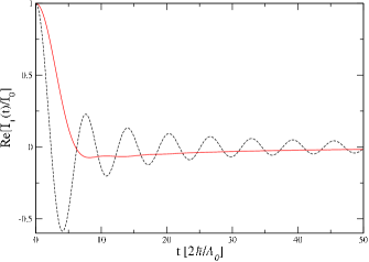
Figure 2: $\mathrm{Re}\left[I_{+}(t)/I_{0}\right]$ determined numerically from Eq. (60). For $d=3$, $m=1$ (solid line), this corresponds to a hydrogen-like $s$-type envelope wave function, and for $d=m=2$ (dashed line), corresponding to a two-dimensional Gaussian envelope wave function. For the hydrogen-like wave function, nuclear spins far from the origin, with small coupling constants, are responsible for the slow (non-oscillatory) asymptotic behavior. In contrast, for the Gaussian envelope wave function nuclear spins near the center, with larger coupling constants, give rise to oscillations in the asymptotic behavior of $I_{+}(t)/I_{0}$.

V Non-Markovian dynamics

In this section we describe a complete calculation for the non-Markovian electron spin dynamics within the Born approximation. In the limit of a fully polarized initial state, our Born approximation applied to $\left\langle S_{+}\right\rangle_{t}$ recovers the exact solution of Ref. Khaetskii et al., 2002a. All results of this section are, however, valid for arbitrary polarization in high magnetic fields when the condition $\left|\Delta\right|\ll 1$ is satisfied. In addition, we find that the remainder term is bounded by the small parameter $\delta$, $\left|R_{X}(t)\right|\leq O(\delta)$, and the stationary limit (long-time average) of the spin can be determined with the much weaker condition $\delta\ll 1$. In zero magnetic field, and for nuclear spin $I=\frac{1}{2}$, the relevant smallness parameter is $\delta=\frac{1}{p^{2}N}$ (see Table 1).

We evaluate the Laplace transforms of (29), (30): $S_{X}(s)=\int_{0}^{\infty}dte^{-st}\left\langle S_{X}\right\rangle_{t},\,\mathrm{Re}[s]>0$, $X=z,+$, to convert the integro-differential equations into a pair of linear algebraic equations which can be solved to obtain

$$S_{z}(s) = \frac{\left\langle S_{z}\right\rangle_{0}+N_{z}(s)}{s+i\Sigma_{zz}(s)},$$ (63)

$$S_{+}(s) = \frac{\left\langle S_{+}\right\rangle_{0}}{s-i\omega_{n}+i\Sigma_{++}(s)}.$$ (64)

When the functions $N_{z}(s),\,\Sigma_{zz}(s),\,\Sigma_{++}(s)$ are known, the Laplace transforms in (63) and (64) can be inverted by evaluating the Bromwich contour integral:

$$\left\langle S_{X}\right\rangle_{t}=\frac{1}{2\pi i}\int_{\gamma-i\infty}^{\gamma+i\infty}ds\mathrm{e}^{st}S_{X}(s),$$ (65)

where all non-analyticities of $S_{X}(s)$ lie to the left of the line of integration. To simplify the calculation, here we specialize to the case of an electron confined to a two-dimensional parabolic quantum dot ($d=m=2$), where the coupling constant integrals can be performed easily to obtain the explicit form for $I_{\pm}(s)$, given in Eq. (42).

Within the Born approximation, $S_{z}(s)$ has six branch points, located at $i\omega_{n},\,i\left(\omega_{n}\pm 1\right),\,-i\omega_{n},\,-i\left(\omega_{n}\pm 1\right)$. We choose the principal branch for all logarithms, defined by $\log(z)=\ln\left|z\right|+i\arg(z)$, where $-\pi<\arg(z)\leq\pi$, in which case there are five poles in general. Three of these poles are located on the imaginary axis and two have finite negative real part. $S_{+}(s)$ has three branch points (at $s=0,\,\pm i$), and three poles in general. One pole has finite negative real part and two are located on the imaginary axis.

Figure 3: The closed contour $C$ used for evaluation of the inverse Laplace transforms of $S_{X}(s)$, $X=z,+$. All non-analyticities of $1/D(s)$ are shown above, where $D(s)$ is given in Eq. (74). Branch cuts are indicated by dashed lines, branch points by crosses, and open circles mark pole positions. The contour $C_{\alpha}$ surrounds the branch cut extending from branch point $\gamma_{\alpha}=\alpha i$, $\alpha=0,+,-$. When the arc that closes the contour in the negative-real half-plane is extended to infinity, $C_{B}$ becomes the Bromwich contour. The pole at $s_{2}$ has finite real part and is present for $b\neq 0$. The poles at $s_{1}$ and $s_{3}$ are always located on the imaginary axis.

Applying the residue theorem to the integral around the closed contour $C$ shown in Fig. 3, $\frac{1}{2\pi i}\oint_{C}dse^{st}S_{X}(s)$, gives

$$\left\langle S_{X}\right\rangle_{t}+\beta^{X}(t) = \sum_{i}P_{i}^{X}(t),\,\,\,\,\,X=z,+,$$ (66)

where the pole contribution $P_{i}^{X}(t)=\mathrm{Res}\left[e^{st}S_{X}(s),\,s=s_{i}\right]$ is the residue from the pole at $s_{i}$, and the branch cut contributions are

$$\beta^{z}(t) = \sum_{\alpha=0,+,-}\frac{1}{\pi}\mathrm{Im}\left[e^{-i\omega_{n}t}K_{\alpha}^{z}(t)\right],$$ (67)

$$\beta^{+}(t) = \frac{1}{2\pi i}\sum_{\alpha=0,+,-}K_{\alpha}^{+}(t),$$ (68)

with branch cut integrals given by

$$K_{\alpha}^{z}(t) = \int_{C_{\alpha}}dse^{st}S_{z}\left(s-i\omega_{n}\right),$$ (69)

$$K_{\alpha}^{+}(t) = \int_{C_{\alpha}}dse^{st}S_{+}\left(s\right).$$ (70)

The contour $C_{\alpha}$ runs from $\gamma_{\alpha}-\infty+i\eta$, around $\gamma_{\alpha}$, and back to $\gamma_{\alpha}-\infty-i\eta$, where $\eta\to 0^{+}$. The branch points are given by $\gamma_{\alpha}=\alpha i,\,\alpha=0,+,-$, as illustrated in Fig. 3. In (67) we have used the fact that the branch cut integrals for $S_{z}(s)$ come in complex conjugate pairs, since $S_{z}(s^{*})=\left[S_{z}(s)\right]^{*}$. This relationship follows directly from the definition for the Laplace transform of the real quantity $\left\langle S_{z}\right\rangle_{t}$.

Combining Eqs. (32), (34), (35), and (42) to obtain $\Sigma_{zz}^{(2)}(s-i\omega_{n})$, and expanding in $\frac{1}{\omega_{n}}$ gives

$$\Sigma_{zz}^{(2)}(s-i\omega_{n})=\Sigma_{++}^{(2)}(s)+\frac{\Delta}{4}(c_{+}+c_{-})+O\left(\delta\right),$$ (71)

where we recall $\Delta=\frac{N}{\omega_{n}}$ and $\delta=\frac{N}{\omega_{n}^{2}}$. The term $\frac{\Delta}{4}\left(c_{+}+c_{-}\right)$ gives rise to a small shift in the effective magnetic field experienced by $\left\langle S_{z}\right\rangle_{t}$. To simplify the presentation, this shift is neglected, but it could easily be included by introducing a slight difference in the denominators of $S_{z}(s)$ and $S_{+}(s)$. This gives

$$S_{z}(s-i\omega_{n}) \simeq \frac{\left\langle S_{z}\right\rangle_{0}+N_{z}^{(2)}(s-i\omega_{n})}{D(s)},$$ (72)

$$S_{+}(s) = \frac{\left\langle S_{+}\right\rangle_{0}}{D(s)}.$$ (73)

The denominator $D(s)=s-i\omega_{n}+i\Sigma_{++}^{(2)}(s)$ and numerator $N_{z}^{(2)}(s-i\omega_{n})$ are given explicitly by

$$D(s) = s-ib^{\prime}+Ns\left[c_{-}\log(s-i)+c_{+}\log(s+i)-(c_{+}+c_{-})\log(s)\right],$$ (74)

$$N_{z}^{(2)}(s-i\omega_{n}) = -\frac{\Delta}{2}(c_{+}+c_{-})-i\Delta\frac{s}{2}\left[c_{+}\log(s+i)-c_{-}\log(s-i)+(c_{-}-c_{+})\log(s)\right]+O\left(\delta\right).$$ (75)

The branch cuts and poles of $S_{z}(s-i\omega_{n})$ and $S_{+}(s)$, as given in Eqs. (72) and (73), are shown in Fig. 3. We note that different analytic features will produce different types of dynamic behavior after the inversion integral has been evaluated. The branch cut contributions $\beta^{X}(t)$ have long-time tails that are non-exponential. Poles with finite negative real part will give rise to exponential decay. Poles on the imaginary axis away from the origin will lead to undamped oscillations, and a pole at the origin will give a constant residue, independent of time. The rest of this section is divided accordingly, describing each type of contribution to the total time evolution of $\left\langle S_{X}\right\rangle_{t}$.

V.1 Non-exponential decay

The contribution to $K_{\alpha}^{X}(t)$ circling each branch point $\gamma_{\alpha}$ is zero, so the branch cut integrals can be rewritten as

$$K_{\alpha}^{X}(t)=e^{\gamma_{\alpha}t}\int_{0}^{\infty}dxe^{-xt}\xi_{X}(x,\gamma_{\alpha})$$ (76)

where

$$\xi_{X}(x,\gamma_{\alpha})=\lim_{\eta\to 0^{+}}\left[S_{X}(s_{\alpha}^{X}(x)+i\eta)\right.\\ -\left.S_{X}(s_{\alpha}^{X}(x)-i\eta)\right],$$ (77)

with

$$s_{\alpha}^{X}(x)=-x+\gamma_{\alpha}+\left\{\begin{array}[]{c}-i\omega_{n},\,\,X=z\\ 0,\,\,X=+\end{array}\right..$$ (78)

The form of $K_{\alpha}^{X}(t)$ in Eq. (76) suggests a direct procedure for evaluating the long-time asymptotics of the branch cut contributions. For long times, the integrand of (76) is cut off exponentially at $x\sim\frac{1}{t}\to 0$. To find the asymptotic behavior, we find the leading $x$-dependence of $\xi_{X}(x,\gamma_{\alpha})$ for $x\to 0^{+}$. We substitute this into (76), and find the first term in an asymptotic expansion of the remaining integral. The leading-order long-time asymptotics obtained in this way for all branch cut integrals $K_{\alpha}^{X}(t)$ are given explicitly in Appendix E. When $b^{\prime}=0$, the denominator $D(s)\to 0$ when $s\to 0$, and the dominant asymptotic behavior comes from $K_{0}^{X}(t\to\infty)\propto\frac{1}{\ln t}$. For $b^{\prime}\neq 0$, $D(s)$ remains finite at the $s=0$ branch point and the dominant long-time contributions come from $K_{\pm}^{X}(t\to\infty)\propto\frac{1}{t\ln^{2}t}$. In zero magnetic field, the leading-order term in the asymptotic expansion is dominant for times $t\gg 1$, but in a finite magnetic field, the leading term only dominates for times $t\gg e^{\left|b^{\prime}\right|/N}$. In summary,

$$\beta^{X}(t\gg 1) \propto \frac{1}{\ln t},\,\,\,\,\,\,\,\,\,\,\,\,b^{\prime}=0,$$ (79)

$$\beta^{X}(t\gg e^{\left|b^{\prime}\right|/N}) \propto \frac{1}{t\ln^{2}t},\,\,\,\,\,\,\,\,\,\,b^{\prime}\neq 0.$$ (80)

This is in agreement with the exact resultKhaetskii et al. (2002b) for a fully-polarized system of nuclear spins $I=\frac{1}{2}$ in a two-dimensional quantum dot. This inverse logarithmic time dependence cannot be obtained from the high-field solutions of Section IV. The method used here to evaluate the asymptotics of the Born approximation therefore represents a nontrivial extension of the exact solution to a nuclear spin system of reduced polarization, but with $\left|\Delta\right|<1$ (see Table 1).

The branch cut integrals can be evaluated for shorter times in a way that is asymptotically exact in a high magnetic field. To do this, we expand the integrand of Eq. (76) to leading nontrivial order in $\frac{1}{\omega_{n}}$, taking care to account for any singular contributions. For asymptotically large positive magnetic fields, we find (see Appendix E):

$$\sum_{\alpha}K_{\alpha}^{X}(t)\sim-i2\pi\delta\left(C_{-}^{X}I_{+}(t)+C_{+}^{X}I_{-}(t)\right)\\ -\frac{C_{-}^{X}}{Nc_{-}^{2}}e^{-z_{0}t}$$ (81)

with coefficients $C_{\pm}^{X}$ given in (53) and in the above,

$$z_{0} = x_{0}-i\epsilon(x_{0}),$$ (82)

$$x_{0} = \frac{\omega_{n}}{2\pi Nc_{-}},$$ (83)

$$\epsilon(x) = \frac{x}{2\pi c_{-}N}+\frac{c_{+}+c_{-}}{4\pi c_{-}x}.$$ (84)

In high magnetic fields, we will show that the exponential contribution to Eq. (81) cancels with the contribution from the pole at $s_{2}$, $P_{2}^{X}(t)$. We stress that this result is only true in the high-field limit $\frac{\left|b^{\prime}\right|}{N}\gg 1$, where the asymptotics are valid.

V.2 Exponential decay

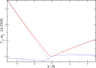
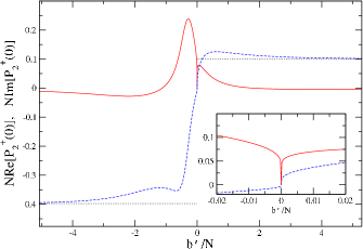
Figure 4: Top: numerically determined rate $\Gamma_{2}$ (solid line) and frequency renormalization $\omega_{2}$ (dashed line) as a function of magnetic field $b^{\prime}/N$. Bottom: $N\mathrm{Re}\left[P_{2}^{+}(0)\right]$ (solid line) and $N\mathrm{Im}\left[P_{2}^{+}(0)\right]$ (dashed line) as a function of magnetic field for the initial state $\left\langle S_{+}\right\rangle_{0}=\left\langle S_{x}\right\rangle_{0}=\frac{1}{2}$. The dotted lines give the asymptotics for high magnetic fields from Eqs. (87), (88), and (89). The parameters used were $p=0.6$, $N=10^{5}$, $I=\frac{1}{2}$.

When $b^{\prime}=0$, there are no poles with finite real part. For $b^{\prime}\neq 0$, a pole (at $s_{2}$ in Fig. 3) emerges from the branch point at $s=0$. The pole contribution $P_{2}^{X}(t)$ decays exponentially with rate $\Gamma_{2}=-\mathrm{Re}[s_{2}]$, and has an envelope that oscillates at a frequency determined by $\omega_{2}=\mathrm{Im}[s_{2}]$:

$$P_{2}^{z}(t) = e^{-\Gamma_{2}t}e^{-i(\omega_{n}-\omega_{2})t}P_{2}^{z}(0)$$ (85)

$$P_{2}^{+}(t) = e^{-\Gamma_{2}t}e^{i\omega_{2}t}P_{2}^{+}(0).$$ (86)

Setting $s_{2}=-\Gamma_{2}+i\omega_{2}$, we find the decay rate $\Gamma_{2}$, frequency renormalization $\omega_{2}$, and amplitudes of these pole contributions from asymptotic solutions to the pair of equations $\mathrm{Re}[D(s_{2})]=\mathrm{Im}[D(s_{2})]=0$ and $P_{2}^{X}(0)=\mathrm{Res[S_{X}(s)},s=s_{2}]$ for high and low magnetic fields $b^{\prime}$. $\Gamma_{2},\,\omega_{2}$, and $P_{2}^{X}(0)$ have the asymptotic field dependences (for high magnetic fields $b^{\prime}\gg N$):

$$\Gamma_{2} \sim \pm\frac{\omega_{n}}{2\pi Nc_{\mp}},\,\,\,\,\omega_{n}\gtrless 0,$$ (87)

$$\omega_{2} \sim \pm\frac{\Gamma_{2}}{2\pi c_{\mp}N}\pm\frac{c_{+}+c_{-}}{4\pi c_{\mp}\Gamma_{2}},\,\,\,\,\omega_{n}\gtrless 0,$$ (88)

$$P_{2}^{X}(0) \sim \frac{C_{\mp}^{X}/c_{\mp}}{1\mp i2\pi Nc_{\mp}},\,\,\,\,\omega_{n}\gtrless 0.$$ (89)

Although it does not correspond to the perturbative regime, it is interesting to consider the behavior of the exponentially decaying pole contribution $P_{2}^{X}(t)$ in the limit $b^{\prime}\to 0$, since the Hamiltonian $\mathcal{H}$ in Eq. (1) is known to be integrable for $B_{z}=0$ ($b^{\prime}=0$).Schliemann et al. (2003) For vanishing positive magnetic fields $\left(b^{\prime}\to 0^{+}\right)$, with logarithmic corrections in $\frac{b^{\prime}}{Eb_{0}}$, where $b_{0}=N(c_{+}+c_{-})$ and $E=\exp\left\{1+O\left(\frac{1}{N}\right)\right\}$:

$$\Gamma_{2} \sim \frac{\zeta b^{\prime}/b_{0}}{\ln^{2}\left(\frac{b^{\prime}}{Eb_{0}}\right)},$$ (90)

$$\omega_{2} \sim -\frac{b^{\prime}/b_{0}}{\ln\left(\frac{b^{\prime}}{Eb_{0}}\right)},$$ (91)

$$P_{2}^{+}(0) \sim -\frac{\left\langle S_{+}\right\rangle_{0}}{N(c_{+}+c_{-})\ln\left(\frac{b^{\prime}}{b_{0}}\right)},$$ (92)

$$P_{2}^{z}(0) \sim -\frac{\left\langle S_{z}\right\rangle_{0}-\left(c_{+}+c_{-}\right)/2pI}{N(c_{+}+c_{-})\ln\left(\frac{b^{\prime}}{b_{0}}\right)},$$ (93)

where $\zeta=\frac{\pi c_{-}}{c_{+}+c_{-}}$. The exponentially decaying contribution vanishes only when $b^{\prime}=0$, and does so in an interval that is logarithmically narrow. We have determined the rate, frequency renormalization, and amplitude of the pole contribution $P_{2}^{+}(t)$ numerically. The results are given in Fig. 4 along with the above asymptotics for high magnetic fields, $\left|b^{\prime}\right|\gg N$.

V.3 Undamped oscillations

The point $s_{1}$ in Fig. 3 corresponds to $s=0$ for $S_{z}(s)$, so undamped oscillations in $\left\langle S_{z}\right\rangle_{t}$ arise only from the pole at $s_{3}$:

$$P_{3}^{z}(t)=e^{-i(\omega_{n}-\omega_{3})t}P_{3}^{z}(0).$$ (94)

Both poles on the imaginary axis give undamped oscillations in $\left\langle S_{+}\right\rangle$:

$$P_{1}^{+}(t)+P_{3}^{+}(t)=e^{i\omega_{1}t}P_{1}^{+}(0)+e^{i\omega_{3}t}P_{3}^{+}(0).$$ (95)

For high magnetic fields, $\left|b^{\prime}/N\right|\gg 1$,

$$\omega_{1/3} \sim b^{\prime}+2pIN=\omega_{n},\,\,\,\,\,b^{\prime}\gtrless 0,$$ (96)

$$\omega_{3/1} \sim \mp 1\mp f_{\pm}\exp\left(-\frac{\left|b^{\prime}\right|}{c_{\pm}N}\right),\,\,\,\,\,b^{\prime}\gtrless 0,$$ (97)

where $f_{\pm}=\left(\frac{1}{2}\right)^{\left(\frac{c_{\mp}}{c_{\pm}}\right)}\left(1+O\left(\frac{1}{N}\right)\right)$. The frequency in Eq. (96) corresponds to a simple precession of the electron spin in the sum of the magnetic and Overhauser fields. The second frequency, Eq. (97), describes the back-action of the electron spin, in response to the slow precession of the nuclear spins in the effective field of the electron.

For large $b^{\prime}$, the pole corresponding to simple precession is dominant, while the other has a residue that vanishes exponentially:

$$P_{1/3}^{+}(0) \sim \frac{\left\langle S_{+}\right\rangle_{0}}{1+\frac{1}{2}(c_{+}+c_{-})\delta},\,\,\,\,\,b^{\prime}\gtrless 0,$$ (98)

$$P_{3/1}^{+}(0) \sim \frac{\left\langle S_{+}\right\rangle_{0}}{Nc_{\pm}}f_{\pm}\exp\left(-\frac{\left|b^{\prime}\right|}{c_{\pm}N}\right),\,\,\,\,\,b^{\prime}\gtrless 0,$$ (99)

$$P_{3}^{z}(0) \sim \frac{b^{\prime}}{2c_{+}N}f_{+}\exp\left(-\frac{\left|b^{\prime}\right|}{c_{+}N}\right),\,\,\,\,\,b^{\prime}>0.$$ (100)

When the magnetic field $b^{\prime}$ compensates the nuclear Overhauser field $\left[h_{z}\right]_{nn}$ ($\omega_{n}\approx 0$, the usual ESR resonance condition in the rotating frame), the poles at points $s_{1}$ and $s_{3}$ have equal weight, and are the dominant contribution to the electron spin dynamics. Since the resonance condition corresponds to the strongly non-perturbative regime, $\left|\Delta\right|\gg 1$, we delay a detailed discussion of the resonance until Section VII.

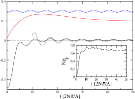
Figure 5: Contributions to the inverse Laplace transform of $\left\langle S_{z}\right\rangle_{t}$. We show the envelopes of the rapidly oscillating functions $2N\mathrm{Re}\left[P_{3}^{z}(t)\right]+0.3$, $2N\mathrm{Re}\left[P_{2}^{z}(t)\right]+0.2$, and $-N\beta^{z}(t)$, determined numerically. The long-time asymptotics of $\beta^{z}(t)$ from Appendix E are also shown (dashed line). The sum of all contributions is used to obtain the population of the spin-up state: $\rho_{\uparrow}(t)=\frac{1}{2}+\left\langle S_{z}\right\rangle_{t}$ (inset). The electron spin begins down: $\left\langle S_{z}\right\rangle_{0}=-\frac{1}{2}$. Other parameters were $I=\frac{1}{2}$, $N=10^{5}$, $b^{\prime}=\frac{N}{2}$ (this value of $b^{\prime}$ gives, e.g., $B_{z}\simeq 1\mathrm{T}$ in GaAs), and $p=0.6$. The time $t$ is given in units of $\frac{2\hbar}{A_{0}}=\frac{2N\hbar}{A}$ for $d=m=2$ in Eq. (43) ($\frac{2N\hbar}{A}\simeq 1\mathrm{\mu s}$ in GaAs). These values correspond to the weakly perturbative regime, with $\Delta=\frac{10}{11}<1$. Note that $\rho_{\uparrow}(t)\lesssim\frac{1}{N}$ for all times.

V.4 Stationary limit

The contribution to $\left\langle S_{z}\right\rangle_{t}$ from the pole at $s=0$ gives the long-time average value $\overline{\left\langle S_{z}\right\rangle}_{\infty}$, which we define as the stationary limit:

$$\overline{\left\langle S_{z}\right\rangle}_{\infty}=\lim_{T\to\infty}\frac{1}{T}\int_{0}^{T}\left\langle S_{z}\right\rangle_{t}dt=\lim_{s\to 0}sS_{z}(s).$$ (101)

Within the Born approximation, we find

$$\overline{\left\langle S_{z}\right\rangle}_{\infty}=\frac{\left\langle S_{z}\right\rangle_{0}+pI\delta+O\left(\frac{N}{\omega_{n}^{4}}\right)}{1+(c_{+}+c_{-})\delta+O\left(\frac{N}{\omega_{n}^{4}}\right)}.$$ (102)

The result in Eq. (102) follows from Eqs. (63), (31), (32), (34), (35), and (37) by expanding the numerator and denominator in $\frac{1}{\omega_{n}}$, using the coupling constants $A_{k}=2e^{-k/N}$ and performing the continuum limit. $\overline{\left\langle S_{z}\right\rangle}_{\infty}$ gives the stationary level populations for spin-up and spin-down: $\bar{\rho}_{\uparrow/\downarrow}=\frac{1}{2}\pm\overline{\left\langle S_{z}\right\rangle}_{\infty}$, which would be fixed by the initial conditions in the absence of the hyperfine interaction. This difference in $\bar{\rho}_{\uparrow/\downarrow}$ from the initial values can be regarded as leakage due to the nuclear spin environment. We note that the stationary value depends on the initial value $\left\langle S_{z}\right\rangle_{0}$, from which it deviates only by a small amount of order $\delta$. This means, in particular, that the system is non-ergodic. We will find that corrections to $\overline{\left\langle S_{z}\right\rangle}_{\infty}$ at fourth order in the flip-flop terms will be of order $\delta^{2}$, so that the stationary limit can be determined even outside of the perturbative regime $\left|\Delta\right|<1$, in zero magnetic field, where $\delta=\frac{1}{p^{2}N}$ for $I=\frac{1}{2}$, provided $p\gg\frac{1}{\sqrt{N}}$.

V.5 Summary

The results of this section for low magnetic fields are summarized in Fig. 5, which corresponds to the weakly perturbative case, $\left|\Delta\right|\lesssim 1$, and displays all of the dynamical features outlined here.

In very high magnetic fields $\left(b^{\prime}\gg N\right)$, corresponding to the strongly perturbative case, we combine Eqs. (81), (96), (98), and (102) to obtain the asymptotic forms to leading order in $\frac{1}{\omega_{n}}$:

$$\left\langle S_{+}\right\rangle_{t} \sim \sigma_{+}^{\mathrm{osc}}(t)+\sigma_{+}^{\mathrm{dec}}(t),$$ (103)

$$\left\langle S_{z}\right\rangle_{t} \sim \overline{\left\langle S_{z}\right\rangle}_{\infty}+\sigma_{z}^{\mathrm{dec}}(t),$$ (104)

where the functions $\sigma_{+}^{\mathrm{osc}}(t),\,\sigma_{+}^{\mathrm{dec}}(t),\,\overline{\left\langle S_{z}\right\rangle}_{\infty},\,\sigma_{z}^{\mathrm{dec}}(t)$, given in Eqs. (46), (47),(49), and (50) are evaluated for $d=m=2$. We stress that $\sigma_{X}^{\mathrm{dec}}(t)\propto\delta\ll 1$ is a small fraction of the total spin. The exponentially decaying contribution from $P_{2}^{X}(t)$ is canceled by the exponential part of the high-field branch cut, given in Eq. (81). This result is in agreement with the high-field asymptotic forms found earlier in Section IV. Numerical results for the level populations $\rho_{\uparrow/\downarrow}(t)=\frac{1}{2}\pm\left\langle S_{z}\right\rangle_{t}$ are given in Fig. 6 along with the above asymptotic forms. The secular term that appeared at lowest order in the standard perturbation expansion of $\left\langle S_{+}\right\rangle_{t}$ is again absent from the result obtained here via the GME. At fourth order, $t$-linear terms also appear in the standard perturbation expansion for the longitudinal spin $\left\langle S_{z}\right\rangle_{t}$.Khaetskii et al. (2002a, b) Due to the numerator term $N_{z}(s)$ in the expression for $S_{z}(s)$ (Eq. (63)), it is not clear if all divergences have been re-summed for $\left\langle S_{z}\right\rangle_{t}$ in the perturbative expansion of the self-energy. This question is addressed in Sec. VII with an explicit calculation of the fourth-order spin dynamics.

In the next section we propose a method that could be used to probe the non-Markovian electron spin dynamics experimentally.

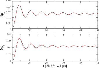
Figure 6: Envelope of the time-dependent spin level populations in high magnetic fields. We give results from numerical inversion of the Laplace transform (solid line) and the asymptotic branch cut integral for high magnetic fields combined with numerical results for the pole positions and residues (dashed line). Top: spin-down level population when the electron begins in the up state, along the nuclear spin polarization direction ($\left\langle S_{z}\right\rangle_{0}=\frac{1}{2}$). Bottom: spin-up population for an electron that begins pointing in the opposite direction ($\left\langle S_{z}\right\rangle_{0}=-\frac{1}{2}$). The parameters used were $N=10^{5}$, $p=0.6$, $I=\frac{1}{2}$ and $b^{\prime}=8N$, corresponding to a field of $B_{z}=14\,\mathrm{T}$ in GaAs.

VI Measurement

In high magnetic fields $(b^{\prime}\gg N)$, the decaying fraction of the electron spin is very small $\left(O\left(\delta\approx\frac{N}{b^{\prime 2}}\right)\right)$. Nevertheless, the large separation between the hyperfine interaction decay time ($\tau_{\mathrm{hf}}=\frac{2\hbar}{A_{0}}\approx 1\mathrm{\mu s}$) and the dipolar correlation time ($\tau_{\mathrm{dd}}\approx 100\,\mathrm{\mu s}$ in GaAs) of the nuclear spins should allow one to obtain valuable information about the electron spin decay from a conventional spin echo technique applied to an ensemble of electron spins.

In principle, the non-Markovian electron spin dynamics should be visible in the electron spin echo envelope obtained by applying the conventional Hahn echo sequence:Slichter (1980) $\frac{\pi}{2}-\tau-\pi_{x}-\tau-\mathrm{ECHO}$ to a large ensemble of electron spins. This can be done by conventional means for an electron trapped at donor impurities in a solid,Tyryshkin et al. (2003) or from a measurement of transport current through a quantum dot.Engel and Loss (2001, 2002) The effect of this echo sequence can be summarized as follows. The electron spins are initially aligned along the external magnetic field $B_{z}$. At time $t=0$ the spins are tipped into the $x-y$ plane with an initial $\frac{\pi}{2}$-pulse. Each spin precesses in its own local effective magnetic field $\omega_{n}$. The phase factor $e^{i\omega_{n}t}$ winds in the “forward” direction for a time $\tau$. The sign of $\omega_{n}$ (direction of the local magnetic field) is then effectively reversed with a $\pi$-pulse along the $x$-axis: $\omega_{n}\to-\omega_{n}$. The phase factor $e^{-i\omega_{n}t}$ unwinds in the following time interval $\tau$, and the electron spin magnetization refocuses to give an echo when the phase factor $e^{-i\omega_{n}2\tau}=1$ simultaneously for all spins in the ensemble. As is usually assumed, we take the pulse times and measurement time during the echo to be negligible.Slichter (1980) The spin echo envelope gives the ensemble magnetization (the electron spin expectation value) at the time of the echo as a function of the free evolution time $2\tau$ before the echo. We note that the decaying fraction of $\left\langle S_{z}\right\rangle_{t}$, $\sigma_{z}^{\mathrm{dec}}(t)$, also precesses with the phase factor $e^{i\omega_{n}t}$ (see Eq. (50)), so the same pulse sequence can also be applied to measure the decay of the longitudinal spin, omitting the initial $\frac{\pi}{2}$-pulse. The Hahn echo envelope should show a small initial decay by $O(\delta)$ in a time scale $\tau_{\mathrm{hf}}$ due to the contact hyperfine interaction, followed by a slow decay due to spectral diffusionde Sousa and S. Das Sarma (2003a, b); Abe et al. (2004) with a time scale $\tau_{\mathrm{dd}}\approx 10^{-4}\,\mathrm{s}$. We note that a rapid initial decay of the Hahn echo envelope has been measured for natural $\mathrm{Si:P}$, but is absent in isotopically enriched $\mathrm{{}^{28}Si:P}$, in which no nuclei carry spin.Fanciulli et al. (2003)

The fraction of the spin that decays in the time $\tau_{\mathrm{hf}}$ is small, of order $\delta$, in the perturbative regime. It may be difficult to detect this small fraction using the conventional Hahn echo. This problem can be reduced by taking advantage of the quantum Zeno effect, using the Carr-Purcell-Meiboom-Gill (CPMG) echo sequence $\frac{\pi}{2}-\left(\tau-\pi_{x}-\tau-\mathrm{ECHO}-\tau-\pi_{-x}-\tau-\mathrm{ECHO}\right)_{\mathrm{repeat}}$. During each free evolution time between echoes, the electron decays by an amount of order $\delta$. At each echo, a measurement of the electron spin magnetization is performed. For a large ensemble of electron spins, this measurement determines the state $\rho_{S}$ of the electron spin ensemble, forcing the total system into a direct product of electron and nuclear states, as in Eq. (10). Repetition of such measurement cycles will then reveal the spin decay due to the hyperfine interaction (by order $\delta$ after each measurement) until the magnetization envelope reaches its stationary value. If the electron spin decays during the free evolution time due to spectral diffusion with a Gaussian envelope, then we require the condition $\left(\frac{2\tau}{\tau_{dd}}\right)^{2}\ll\delta\ll 1$ for the effect of spectral diffusion to be negligible compared to the effect of the hyperfine interaction. The non-Markovian remainder term gives the total change in electron spin that has occurred during the free evolution time $2\tau$: $\left.R_{X}(2\tau)\right|_{e^{\pm i\omega_{n}2\tau}=1}=\left.\left\langle S_{X}\right\rangle_{2\tau}-\left\langle S_{X}\right\rangle_{0}\right|_{e^{\pm i\omega_{n}2\tau}=1}=M_{X}(2\tau)-M_{X}(0)$, where $M_{X}(t)$ is the CPMG magnetization envelope. In high magnetic fields, and when there are many echoes before the magnetization envelope decays, the CPMG magnetization envelopes $M_{X}(t)$ will therefore obey the differential equations

$$\frac{d}{dt}M_{X}(t)=\left.\frac{R_{X}(2\tau)}{2\tau}\right|_{\left\langle S_{X}\right\rangle_{0}=M_{X}(t),\,e^{\pm i\omega_{n}2\tau}=1},\,\,\,\,\,X=+,z,$$ (105)

where the high-field expressions for $R_{X}(t)$, given in Eqs. (58) and (59), should be used. Thus, the decay rate of the CPMG echo envelope $M_{X}$, as a function of the free evolution time $2\tau$, is a direct probe of the non-Markovian remainder term $R_{X}(t)$.

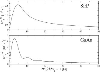
Figure 7: Longitudinal decay rate $\frac{1}{T_{1}^{M}}$ of the CPMG echo envelope as a function of the free evolution time $2\tau$ between $\pi$-pulses for an electron trapped at a phosphorus donor impurity in Si:P (top) and in a two-dimensional GaAs quantum dot (bottom). The free evolution time is given in units of $\frac{2\hbar}{A_{0}}\approx\frac{2N\hbar}{A}$ (the equality is exact for $d=m=2$ in Eq. (43)). In a GaAs quantum dot containing $N=10^{5}$ nuclei or for an electron trapped at a shallow donor impurity in Si:P with $N=100$ nuclear spins within one Bohr radius, $\frac{2N\hbar}{A}\approx 1\,\mu\mathrm{s}$. We have used $I=\frac{1}{2}$, $p=0.6$, and magnetic field values from Table 2 to determine the frequency units on the vertical axis.

Since the magnetization envelopes $M_{X}(t)$ are found as the result of an ensemble measurement, it is necessary to perform an average over different nuclear initial states $\left|n\right\rangle$ that may enter into the solutions to Eq. (105). The local field-dependent phase factors have been removed by the echo sequence, so the only effect of the ensemble average is to average over $\delta=\frac{N}{\omega_{n}^{2}}$ and $c_{\pm}$, which appear in the overall amplitude of $\frac{d}{dt}M_{X}(t)$. The relative fluctuations in these quantities are always suppressed by the factor $\frac{1}{\sqrt{N}}$ for a large nuclear spin system.

In the high-field limit, we find the longitudinal and transverse magnetization envelopes $M_{z}(t)$ and $M_{+}(t)$ decay exponentially with time constants $T_{1}^{M}$ and $T_{2}^{M}=2T_{1}^{M}$, respectively. $M_{+}(t)$ decays to zero, and $M_{z}(t)$ decays to the limiting value

$$M_{z}(\infty)=\frac{1}{2}\frac{c_{-}-c_{+}}{c_{-}+c_{+}}=\frac{pI}{c_{-}+c_{+}}.$$

For nuclear spin $I=\frac{1}{2}$, $M_{z}(\infty)=\frac{p}{2}$, i.e., the electron magnetization acquires the polarization of the nuclear spin bath. However, since $c_{\pm}\propto I^{2}$, $M_{z}(\infty)\to 0$ in the large-spin limit. Thus, a larger fraction of the electron spin decays in the limit of large nuclear spin. We give plots of the longitudinal spin decay rate for $M_{z}(t)$, $\frac{1}{T_{1}^{M}}$, as a function of the free evolution time $2\tau$ for two types of envelope wave function in Fig. 7. These plots have been determined by integrating Eq. (105) using the high-field expression for $R_{z}(t)$ given in Eq. (59). No ensemble averaging has been performed to generate these plots. When $2\tau\ll\tau_{\mathrm{hf}}$, the envelope decay rate increases as a function of $2\tau$ as more of the electron spin is allowed to decay before each measurement. The rates reach a maximum at some time $2\tau\approx\tau_{\mathrm{hf}}$, and for $2\tau\gg\tau_{\mathrm{hf}}$, the electron spin saturates at its stationary value and the envelope decay rates $\propto\frac{1}{2\tau}$ are determined only by the free evolution time. Note that there are slow oscillations in the CPMG decay rate for an electron in a GaAs quantum dot, with a Gaussian wave function, but none for an electron trapped at a donor impurity in Si:P.

VII Beyond Born

The goal of this section is to address the range of validity of the results obtained in Sec. V. First, we show that the Born approximation for $\left\langle S_{+}\right\rangle_{t}$ recovers the exact solution for $I=\frac{1}{2}$, $p=1$. We then discuss the behavior of the Born approximation near the ESR resonance, where $\omega_{n}\approx 0$. Finally, we consider the expression for $\left\langle S_{z}\right\rangle_{t}$, obtained by including all fourth-order corrections to the reduced self-energy, and show that our expression is well-behaved in the continuum limit.

VII.1 Recovery of the exact solution

When $I=\frac{1}{2}$ and $p=1$, we have $c_{-}=1$ and $c_{+}=0$, which gives $\Sigma_{++}^{(2)}(s)=-\frac{i}{4}\sum_{k}\frac{A_{k}^{2}}{s-i\frac{A_{k}}{2}}$ from Eq. (155). We insert this into (64) and use $\omega_{n}=b^{\prime}+\frac{1}{2}\sum_{k}A_{k}=b^{\prime}+\frac{A}{2}$ to obtain

$$S_{+}(s)=\frac{\left\langle S_{+}\right\rangle_{0}}{s-i\left(b^{\prime}+\frac{A}{2}\right)+\frac{1}{4}\sum_{k}\frac{A_{k}^{2}}{s-iA_{k}/2}}.$$ (106)

The Schrödinger equation for a state of the form $\left|\psi(t)\right\rangle=\alpha_{\Uparrow}(t)\left|\Uparrow\uparrow\uparrow\cdots\right\rangle+\alpha_{\Downarrow}(t)\left|\Downarrow\uparrow\uparrow\cdots\right\rangle+\sum_{k}\beta_{k}(t)\left|\Uparrow\uparrow\cdots\downarrow_{k}\uparrow\cdots\right\rangle$, where the large arrow gives the state of the electron spin and the thin arrows give the states of the nuclear spins, has been written and solved (for a fully polarized nuclear spin initial state, $\beta_{k}(t=0)=0\,\forall\,k$) in Laplace space to find the long-time asymptotic electron spin dynamics previously.Khaetskii et al. (2002b) In Ref. Khaetskii et al., 2002b the symbol $\alpha(t)$ was used in place of $\alpha_{\Downarrow}(t)$. The fully-polarized state $\left|\Uparrow\uparrow\uparrow\cdots\right\rangle$ is an eigenstate of the full Hamiltonian $\mathcal{H}^{\prime}$, so $\alpha_{\Uparrow}(t)=e^{-\frac{i}{2}\left(b^{\prime}+\frac{A}{2}\right)t}\alpha_{\Uparrow}(0)$, which allows us to write $S_{+}(s)=\alpha_{\Uparrow}^{*}(t=0)\alpha_{\Downarrow}\left(s-\frac{i}{2}\left(b^{\prime}+\frac{A}{2}\right)\right)$. We solve the time-dependent Schrödinger equation for $\left|\psi(t)\right\rangle$ in Laplace space, giving

$$\alpha_{\Downarrow}\left(s^{\prime}\right)=\frac{\alpha_{\Downarrow}(t=0^{+})}{s-i\left(b^{\prime}+\frac{A}{2}\right)+\frac{1}{4}\sum_{k}\frac{A_{k}^{2}}{s-iA_{k}/2}},$$ (107)

where $s^{\prime}=s-\frac{i}{2}\left(b^{\prime}+\frac{A}{2}\right)$. Thus, in the limit of full polarization of the nuclear system, the Born approximation applied to $\left\langle S_{+}\right\rangle_{t}$ becomes exact. For a fully polarized nuclear spin system $\left\langle S_{z}\right\rangle_{t}$ is given by the relationship $\left\langle S_{z}\right\rangle_{t}=\frac{1}{2}\left(1-2\left|\alpha_{\Downarrow}(t)\right|\right)=\frac{1}{2}\left(1-2\left|\frac{\left\langle S_{+}\right\rangle_{t}}{\alpha_{\Uparrow}^{*}(t=0)}\right|^{2}\right)$. Unfortunately, this result is not recovered directly from the Born approximation for $\left\langle S_{z}\right\rangle_{t}$, as we will show in the next subsection.

VII.2 Resonance

On resonance, $\omega_{n}=0$, i.e., the external field $b^{\prime}$ compensates the Overhauser field $\left[h_{z}\right]_{nn}$. The resonance is well outside of the perturbative regime, defined by $\left|\Delta\right|=\left|\frac{N}{\omega_{n}}\right|<1$, but we proceed in the hope that the Born approximation applied to the self-energy captures some of the correct behavior in the non-perturbative limit. On resonance, the major contributions to $\left\langle S_{z}\right\rangle_{t}$ come from three poles, at $s=0$, $s=s_{3}$, and $s=s_{3}^{*}$:

$$\left\langle S_{z}\right\rangle_{t}\approx\overline{\left\langle S_{z}\right\rangle}_{\infty}+2\mathrm{Re}\left[P_{3}^{z}(t)\right].$$ (108)

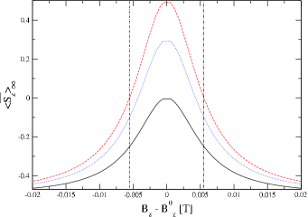
Figure 8: $\overline{\left\langle S_{z}\right\rangle}_{\infty}$ evaluated within Born approximation near the resonance, from Eq. (102) where $B_{z}^{0}=-\frac{pA}{2g^{*}\mu_{B}}$. We have used the value of $A$ for GaAs, $g^{*}=-0.44$, $N=10^{5}$, and $I=\frac{1}{2}$. $\left\langle S_{z}\right\rangle_{0}=-\frac{1}{2}$ for all three curves and results are given for $p=0$ (solid line), $p=\frac{6}{10}$ (dotted line), and $p=1$ (dashed line). The vertical dash-dotted lines indicate the magnetic fields where the relevant smallness parameter is unity: $\left|\delta\right|=1$.

Before applying the continuum limit, the stationary limit for $\left\langle S_{z}\right\rangle_{t}$ is

$$\overline{\left\langle S_{z}\right\rangle}_{\infty}=\frac{\left\langle S_{z}\right\rangle_{0}+\frac{1}{4}\left(c_{-}-c_{+}\right)N_{\mathrm{tot}}}{1+\frac{c_{+}+c_{-}}{2}N_{\ \mathrm{tot}}}.$$ (109)

After applying the continuum limit, $N_{\mathrm{tot}}\to\infty$, we obtain

$$\overline{\left\langle S_{z}\right\rangle}_{\infty}=\frac{1}{2}\frac{c_{-}-c_{+}}{c_{-}+c_{+}}=\frac{pI}{c_{-}+c_{+}}.$$ (110)

For $I=\frac{1}{2}$, $\overline{\left\langle S_{z}\right\rangle}_{\infty}=\frac{p}{2}$, which appears to be an intuitive result. However, evaluating the remaining pole contributions at the resonance, we find, for a two-dimensional quantum dot,

$$2\mathrm{Re}\left[P_{3}(t)\right]=\left[\left\langle S_{z}\right\rangle_{0}-\frac{2pI}{c_{-}+c_{+}}\right]\cos\left(\Omega_{0}t\right)+O\left(\frac{1}{N}\right),$$ (111)

where

$$\Omega_{0}=\sqrt{\frac{N}{2}\left(c_{+}+c_{-}\right)}.$$ (112)

The results in (110) and (111) do not reproduce the exact solution in the limit $p=1$, $I=\frac{1}{2}$, and do not recover the correct $t=0$ value of $\left\langle S_{z}\right\rangle_{t}$. The Born approximation for $\left\langle S_{z}\right\rangle_{t}$, as it has been defined here, breaks down in the strongly non-perturbative limit, although the transverse components are better behaved.

On resonance, the poles at $s_{1}$ and $s_{3}$ are equidistant from the origin, and the major contributions to $\left\langle S_{+}\right\rangle_{t}$ come from these two poles: $\left\langle S_{+}\right\rangle_{t}\approx P_{1}(t)+P_{3}(t)$. Evaluating the residues at these poles,

$$\left\langle S_{+}\right\rangle_{t}=\left\langle S_{+}\right\rangle_{0}\left(1-O\left(\frac{1}{N}\right)\right)\cos\left(\Omega_{0}t\right),$$ (113)

which suggests that a fraction $O\left(\frac{1}{N}\right)$ of the spin undergoes decay, and the rest precesses at a frequency $\Omega_{0}$. When $I=\frac{1}{2}$, and in proper energy units we have $\Omega_{0}=\frac{A}{\sqrt{8N}}$ from Eq. (112). While it does not violate positivity, as in the case of $\left\langle S_{z}\right\rangle_{t}$, this expression should not be taken seriously in general, since this result has been obtained well outside of the perturbative regime. The above does, however, recover the exact solution in the limit $p=1$. We show the stationary limit of $\left\langle S_{z}\right\rangle_{t}$ in Fig. 8, using typical values for an electron confined to a GaAs quantum dot.

VII.3 Fourth-order corrections

The fourth order expansion of the self-energy for $\left\langle S_{z}\right\rangle_{t}$ is given in Appendix A. The discrete expression for the numerator term $N_{z}^{(4)}(s)$ contains second order poles (secular terms). The fourth-order expression for $S_{z}(s)$ inherits these second order poles (see Eq. (63)). When the Laplace transform is inverted, this will result in pole contributions that grow linearly in time. However, when the continuum limit is performed, which is strictly valid for times shorter than $t\approx\sqrt{N}$ (see Appendix C), all poles in $N_{z}^{(4)}(s)$ are replaced by branch cuts. The integrals around the branch cuts can then be performed to obtain a solution for $\left\langle S_{z}\right\rangle_{t}$, valid for times $t\lesssim\sqrt{N}$.

All relevant non-analytic features (branch points and poles) of $S_{z}(s)$ occur in two regions of the complex plane: about the origin $s\approx 0$, and at high frequencies, around $s\approx\pm i\omega_{n}$. Inserting an initial nuclear state $\left|n\right\rangle$ for a large uniform system (see Appendix B), expanding the fourth-order self-energy to leading order in $\frac{1}{\omega_{n}}$ about the points $s=0$ and $s=-i\omega_{n}$, performing the continuum limit, and evaluating the integrals over coupling constants, we obtain (where the overbar and “conj.” indicate complex conjugate for $s$ real):

$$N_{z}^{(4)}(s-i\omega_{n}) \simeq -\frac{\Delta^{2}}{2}\left\{c_{+}c_{-}\left[L_{1}(s)+L_{2}(s)-L_{3}(s)-\mathrm{conj}.\right]+c_{+}^{2}L_{1}(s)-c_{-}^{2}\bar{L}_{1}(s)\right\}$$ (114)

$$\Sigma_{zz}^{(4)}(s-i\omega_{n}) \simeq -N\Delta\left\{c_{+}c_{-}\left[L_{1}(s)+L_{2}(s)-L_{3}(s)+\mathrm{conj}.\right]+c_{+}^{2}L_{1}(s)+c_{-}^{2}\bar{L}_{1}(s)\right\}$$ (115)

$$N_{z}^{(4)}(s) \simeq \frac{\delta^{2}}{2}\left(c_{+}^{2}-c_{-}^{2}\right)\left(\frac{3}{4}+s^{2}L_{4}(s)\right)$$ (116)

$$\Sigma_{zz}^{(4)}(s) \simeq is\delta^{2}\left[3\left(pI\right)^{2}+\left(c_{+}^{2}+c_{-}^{2}+14c_{+}c_{-}\right)s^{2}L_{4}(s)\right]$$ (117)

with coupling constant integrals $L_{i}(s)$ given by

$$L_{1}(s) = \frac{i}{2(s+i)}-\frac{1}{2}\left[\log(s+i)-\log(s)\right]$$ (118)

$$L_{3}(s) = \left[s\log(s+i)-s\log(s)-i\right]^{2}$$ (119)

$$L_{4}(s) = \frac{1}{6}-\frac{1}{6s}\left[s^{3}+3s+2i\right]\left[\log(s+i)-\log(s)\right]-\frac{1}{6s}\left[s^{3}+3s-2i\right]\left[\log(s-i)-\log(s)\right]$$ (120)

and

$$L_{2}(s)=\log(s+i)-\log(s)-i\left[(s+i)\log(s+i)-(s+2i)\log(s+2i)+s\log(s)-(s-i)\log(s-i)\right]\\ +is\int_{s}^{s+i}du\frac{\log(2u-s-i)-\log(2u-s)}{u}.$$ (121)

Noting that $\lim_{s\to 0}s^{2}L_{4}(s)=0$, we find the corrections to the stationary limit for $\left\langle S_{z}\right\rangle_{t}$. At fourth order in the flip-flop terms, this gives

$$\overline{\left\langle S_{z}\right\rangle}_{\infty}=\frac{\left\langle S_{z}\right\rangle_{0}+pI\delta+\frac{3}{8}\left(c_{+}^{2}-c_{-}^{2}\right)\delta^{2}+O\left(\frac{N}{\omega_{n}^{4}}\right)}{1+(c_{+}+c_{-})\delta-3(pI)^{2}\delta^{2}+O\left(\frac{N}{\omega_{n}^{4}}\right)}.$$ (122)

	$\Sigma_{S}\simeq\Sigma_{S}^{(2)}$	$\Sigma_{S}\simeq\Sigma_{S}^{(2)}$	$\Sigma_{S}\simeq\Sigma_{S}^{(2)}$	$\Sigma_{S}\simeq\Sigma_{S}^{(2)}+\Sigma_{S}^{(4)}$	$\Sigma_{S}\simeq\Sigma_{S}^{(2)}$	$\Sigma_{S}\simeq\Sigma_{S}^{(2)}$
	$b^{\prime}=0,$	$b^{\prime}\neq 0,$	$b^{\prime}\neq 0,$	$p\neq 1,$	$\left|\Delta\right|\ll 1,$	$\left|\Delta\right|\ll 1,$
	$\frac{d}{m}=1,$	$\frac{d}{m}=1,$	$\frac{d}{m}=1,$	$\frac{d}{m}=1,$	$\frac{d}{m}<2,$	$\frac{d}{m}\geq 2,$
	$t\gg 1$	$\Gamma_{2}^{-1}\gtrsim t\gg 1$	$t\gg e^{\left|b^{\prime}\right|/N}\gg\Gamma_{2}^{-1}$	$t\gg e^{\left|b^{\prime}\right|/N},\,b^{\prime}\gg 2pIN$	$t\gg 1$	$t\gg 1$
$R_{X}(t)\propto$	$1/\ln t$	$e^{i\omega_{2}t}e^{-\Gamma_{2}t}$	$1/t\ln^{2}t$	$1/t\ln^{3}t$, $X=z$	$(1/t)^{\frac{d}{m}}e^{\pm it}$	$\ln^{\nu}t/t^{2},\,\,\,\,\,\nu=\frac{d}{m}-1$

Table 3: Results for the decaying fraction of the spin $\left(\left|R_{X}(t)\right|<O(\delta)\,\forall\,t\right)$ in various parameter regimes. Results are given for both remainder terms $R_{X}(t),\,X=z,+$, within the Born approximation for the self-energy $\Sigma_{S}\simeq\Sigma_{S}^{(2)}$ and for $R_{z}(t)$ at fourth order in the nuclear spin–electron spin flip-flop terms $\Sigma_{S}\simeq\Sigma_{S}^{(2)}+\Sigma_{S}^{(4)}$ when $p\neq 1$. The first three columns are exact in the limit of full polarization $(p=1)$ of the nuclear spin system, but still may describe the correct electron spin dynamics in the weakly perturbative regime, $\left|\Delta\right|\lesssim 1$. The last two columns give the correct electron spin dynamics in the strongly perturbative regime, $\left|\Delta\right|\ll 1$.

The fourth-order corrections to the self-energy at high frequency ($s\approx-i\omega_{n}$) are suppressed relative to the Born approximation by an additional factor of the smallness parameter $\Delta$, as expected from the analysis given in Appendix A. However, the low-frequency ($s\approx 0$) part of the fourth-order self-energy is suppressed by the much smaller parameter $\delta$. This allows us to determine the stationary limit of $\left\langle S_{z}\right\rangle_{t}$ with confidence even when the magnetic field is small or zero, provided the polarization is sufficiently large. When $b^{\prime}=0$ and $I=\frac{1}{2}$, we have $\delta=\frac{1}{p^{2}N}$, so the stationary limit can be determined whenever $p\gg\frac{1}{\sqrt{N}}$.

It is relatively straightforward to find the time-dependence as $t\to\infty$ for the $S_{z}$ branch cut integrals at fourth order. Neglecting contributions from the branch cuts near $s\simeq 0$, which are suppressed by the factor $\delta^{2}$, and when $p<1$ so that the coefficient $c_{+}\neq 0$ (c.f. Eq. (38)), we find the major contributions at long times come from the branch points at $s=\pm i$, where $L_{2}(s)\propto\log^{2}(s+i)$. For any magnetic field, we find:

$$R_{z}\left(t\to\infty\right)\propto\frac{1}{t\ln^{3}t}.$$ (123)

For $b^{\prime}\gg 2pIN$, this time-dependence will be dominant when $t\gg\exp\left(\frac{\left|b^{\prime}\right|}{N}\right)$. Thus, we find that the fourth-order result has a faster long-time decay than the Born approximation, and that the associated asymptotics are valid at the same times as the Born approximation asymptotics (see Eq. (80)). Thus, higher-order corrections may change the character of the long-time decay in the weakly perturbative regime, where they are not negligible. In contrast, in the strongly perturbative regime $\left|\Delta\right|\ll 1$, the fourth- and higher-order terms are negligible, so the Born approximation dominates for all times $t<\exp\left(\left|b^{\prime}\right|/N\right)$.

VIII Conclusions

We have given a complete analytical description for the dynamics of an electron spin interacting with a nuclear spin environment via the Fermi contact hyperfine interaction. In a large magnetic field, our calculation applies to a nuclear spin system of arbitrary polarization $p$ and arbitrary spin $I$, prepared in an eigenstate of the total $z$-component of the (quantum) nuclear Overhauser field. In the limit of full polarization $p=1$ and nuclear spin $I=\frac{1}{2}$, the Born approximation applied to the self-energy recovers the exact dynamics for $\left\langle S_{+}\right\rangle_{t}$ and $\left\langle S_{z}\right\rangle_{t}$, with all non-perturbative effects. We have shown explicitly that the dynamical behavior we calculate in Born approximation is purely non-Markovian, and can be obtained in the limit of high magnetic fields directly from the remainder term to a Born-Markov approximation. By performing our expansion on the self-energy superoperator, we have re-summed secular divergences that are present in standard perturbation theory at lowest (second) order for the transverse components $\left\langle S_{+}\right\rangle_{t}$ and at fourth and higher order for the longitudinal spin $\left\langle S_{z}\right\rangle_{t}$. For low magnetic fields $b^{\prime}\lesssim N$ , but still within the perturbative regime ($\left|\Delta\right|<1$), the Born approximation for the electron spin shows rich dynamics including non-exponential (inverse logarithm) decay, exponential decay, and undamped oscillations. For high magnetic fields $b^{\prime}\gg N$, and for $\frac{d}{m}<2$, the electron spin shows a power-law decay ($\sim\left(\frac{1}{t}\right)^{\frac{d}{m}}$ in d-dimensions for an isotropic envelope wave function of the form $\psi(r)\propto\exp\left[-\frac{1}{2}\left(\frac{r}{l_{0}}\right)^{m}\right]$) to its stationary value with a time scale $\tau_{\mathrm{hf}}\approx\frac{2N\hbar}{A}$, in agreement with the exact solution for a fully polarized nuclear spin system.Khaetskii et al. (2002a, b) Above a critical ratio, $\frac{d}{m}\geq 2$, the spin decay asymptotics undergo an abrupt change, signaled by a disappearance of slow oscillations in the decay envelope. We have summarized these results in Table 3. We have also suggested a method that could be used to probe the non-Markovian electron spin dynamics directly, using a standard spin-echo technique. We emphasize that the electron spin only decays by some small fraction of its initial value, of order $\delta$ (see Tables 1, 2), and the decay is generically non-exponential at long times (see Table 3). The results of this work may therefore be of central importance to the development of future quantum error correction schemes, which typically assume an exponential decay to zero. The fact that the stationary value of the spin depends on the initial value implies that this system is non-ergodic. Based on this observation, we postulate a general principle, that non-ergodic quantum systems can preserve phase-coherence to a higher degree than systems with ergodic behavior. It would be interesting to explore this connection further.

Appendix A Self-energy expansion

To expand the self-energy superoperator $\Sigma_{S}$ in powers of $L_{V}$, we have found it convenient to work in terms of a superoperator matrix representation. Here we give a brief description of its use and apply it to generate the reduced self-energy at second order in $L_{V}$ for all spin components, and the fourth order for the longitudinal spin.

Any operator $\mathcal{O}$ that acts on both the electron spin and nuclear spin Hilbert spaces can be written in terms of the $2\times 2$ identity, $\sigma_{0}$, and the Pauli matrices $\sigma_{i},\,i=(x,y,z)$:

$$\mathcal{O}=\sum_{i=(0,x,y,z)}c_{i}\sigma_{i}$$ (124)

where the coefficients $c_{i}$ are operators that act only on the nuclear spin space. Equivalently, $\mathcal{O}$ can be written in terms of the operators $\rho_{\uparrow/\downarrow}=\frac{1}{2}\left(\sigma_{0}\pm\sigma_{z}\right)$, $S_{\pm}=\frac{1}{2}\left(\sigma_{x}\pm i\sigma_{y}\right)$, i.e.:

$$\mathcal{O}=k_{\uparrow}\rho_{\uparrow}+k_{\downarrow}\rho_{\downarrow}+k_{+}S_{-}+k_{-}S_{+}$$ (125)

with operators $k_{j}$ that act on the nuclear spin space. We have labeled the coefficients $k_{j}$ in this way so that when $\mathcal{O}=\rho_{S}$ is the electron spin density operator, $k_{\pm}=\left\langle S_{\pm}\right\rangle$. A superoperator $\mathcal{S}$ acting on $\mathcal{O}$ maps it to the operator $\mathcal{O}^{\prime}$ with new coefficients:

$$\mathcal{SO}=\mathcal{O}^{\prime}=k_{\uparrow}^{\prime}\rho_{\uparrow}+k_{\downarrow}^{\prime}\rho_{\downarrow}+k_{+}^{\prime}S_{-}+k_{-}^{\prime}S_{+}.$$ (126)

This allows us to write $\mathcal{O}$ as a vector and $\mathcal{S}$ as a $4\times 4$ matrix, the elements of which are superoperators that act on the nuclear spin space, and are determined by (125) and (126):

$$\vec{\mathcal{O}} = \left(k_{\uparrow},k_{\downarrow},k_{+},k_{-}\right)^{T}$$ (127)

$$\vec{\mathcal{O}}^{\prime} = \left(k_{\uparrow}^{\prime},k_{\downarrow}^{\prime},k_{+}^{\prime},k_{-}^{\prime}\right)^{T},$$ (128)

$\vec{\mathcal{O}}^{\prime}=\left[\mathcal{S}\right]\vec{\mathcal{O}}$ and $k_{\alpha}^{\prime}=\sum_{\beta}\mathcal{S}_{\alpha\beta}k_{\beta}$, where $\alpha,\,\beta=\uparrow,\downarrow,+,-$.

Laplace transforming the reduced self-energy given in (26) yields

$$\Sigma_{S}(s) = -i\mathrm{Tr}_{I}L\frac{1}{s+iQL}L_{V}\rho_{I}(0),$$ (129)

which is expanded in powers of $L_{V}$

$$\frac{1}{s+iQL}=\sum_{k=0}^{\infty}\frac{1}{s+iQL_{0}}\left(-iQL_{V}\frac{1}{s+iQL_{0}}\right)^{k}.$$ (130)

To obtain these higher order terms in the self-energy, we form products of the free propagator $\frac{1}{s+iQL_{0}}$ and the perturbation $QL_{V}$. The free propagator is diagonal in the basis of $\left\{\rho_{\uparrow/\downarrow},\,S_{\pm}\right\}$, and is given in terms of $2\times 2$ blocks by

$$\left[\frac{1}{s+iQL_{0}}\right] = \left(\begin{array}[]{cc}G_{I}^{0}(s)&0\\ 0&G_{I}^{0\prime}(s)\end{array}\right),$$ (133)

where

$$G_{I}^{0}(s) = \left(\begin{array}[]{cc}G_{\uparrow}^{0}(s)&0\\ 0&G_{\downarrow}^{0}(s)\end{array}\right),$$ (136)

$$G_{I}^{0\prime}(s) = \left(\begin{array}[]{cc}G_{+}^{0}(s)&0\\ 0&G_{-}^{0}(s)\end{array}\right).$$ (139)

In the above,

$$G_{\uparrow/\downarrow}^{0}(s) = \frac{1}{s\pm i\frac{Q}{2}L_{\omega}^{-}},$$ (140)

$$G_{\pm}^{0}(s) = \frac{1}{s\mp i\frac{Q}{2}L_{\omega}^{+}},$$ (141)

where we define the new (nuclear spin) Liouvillians by their action on an arbitrary operator $\mathcal{O}$: $L_{\omega}^{\pm}\mathcal{O}=\left[\omega,\mathcal{O}\right]_{\pm},\,\omega=b^{\prime}+h_{z}$. The perturbation term contains only off-diagonal elements when written in terms of $2\times 2$ blocks:

$$\left[QL_{V}\right] = \left(\begin{array}[]{cc}0&V_{I}\\ V_{I}^{\prime}&0\end{array}\right),$$ (144)

where we find

$$V_{I}=\frac{Q}{2}\left(\begin{array}[]{cc}h_{-}^{L}&-h_{+}^{R}\\ -h_{-}^{R}&h_{+}^{L}\end{array}\right),\,\,\,\,\,V_{I}^{\prime}=\frac{Q}{2}\left(\begin{array}[]{cc}h_{+}^{L}&-h_{+}^{R}\\ -h_{-}^{R}&h_{-}^{L}\end{array}\right).$$ (145)

In the above expression, we have introduced superoperators for right and left multiplication:

$$\mathcal{O}^{R}\mathcal{A} = \mathcal{AO}$$ (146)

$$\mathcal{O}^{L}\mathcal{A} = \mathcal{O}\mathcal{A}.$$ (147)

Only even powers of $L_{V}$ can contribute to the final trace over the nuclear system, so we consider a general term in the expansion of the self-energy

$$\left(\left[QL_{V}\right]\left[\frac{1}{s+iQL_{0}}\right]\right)^{2k} = \left(\begin{array}[]{cc}\Sigma_{k}&0\\ 0&\Sigma_{k}^{\prime}\end{array}\right),$$ (150)

$$\Sigma_{k}=\left(V_{I}G_{I}^{0\prime}V_{I}^{\prime}G_{I}^{0}\right)^{k},\,\,\,\,\,\Sigma_{k}^{\prime}=\left(V_{I}^{\prime}G_{I}^{0}V_{I}G_{I}^{0\prime}\right)^{k}.$$ (151)

By inspection of the form of $V_{I}$, $V_{I}^{\prime}$, we find that the $2\times 2$ matrix $\mathrm{Tr}_{I}\Sigma_{k}^{\prime}\rho_{I}(0)$ is diagonal when $\rho_{I}(0)=\left|n\right\rangle\left\langle n\right|$, and $\left|n\right\rangle$ is an eigenstate of $h_{z}$ (as in Eq. (20)), since the off-diagonal components always contain terms proportional to $h_{+}^{2}$ or $h_{-}^{2}$. Thus, to all orders in the perturbation $L_{V}$, the reduced self-energy takes the form

$$\Sigma_{S}(s)=\left(\begin{array}[]{cccc}\Sigma_{\uparrow\uparrow}(s)&\Sigma_{\uparrow\downarrow}(s)&0&0\\ \Sigma_{\downarrow\uparrow}(s)&\Sigma_{\downarrow\downarrow}(s)&0&0\\ 0&0&\Sigma_{++}(s)&0\\ 0&0&0&\Sigma_{--}(s)\end{array}\right).$$ (152)

The number of matrix elements left to calculate can be further reduced with the relationships $\Sigma_{\uparrow\uparrow}(s)=-\Sigma_{\downarrow\uparrow}(s)$, $\Sigma_{\uparrow\downarrow}(s)=-\Sigma_{\downarrow\downarrow}(s)$, which follow directly from the condition $\mathrm{Tr}\dot{\rho}_{S}=0\Rightarrow\dot{\rho}_{\uparrow}(t)=-\dot{\rho}_{\downarrow}(t)$ and the GME $\dot{\rho}_{\alpha}=-i\sum_{\beta=\uparrow,\downarrow}\int_{0}^{t}dt^{\prime}\Sigma_{\alpha\beta}(t-t^{\prime})\rho_{\beta}(t^{\prime}),\,\alpha=\uparrow,\downarrow$. By direct calculation we find

$$\Sigma_{\uparrow\uparrow}^{(2)}(s) = -\frac{i}{4}\sum_{k}\left[h_{-}\right]_{nk}\left[h_{+}\right]_{kn}\left(\frac{1}{s-i\bar{\omega}_{nk}}+\frac{1}{s+i\bar{\omega}_{nk}}\right)$$ (153)

$$\Sigma_{\uparrow\downarrow}^{(2)}(s) = \frac{i}{4}\sum_{k}\left[h_{+}\right]_{nk}\left[h_{-}\right]_{kn}\left(\frac{1}{s-i\bar{\omega}_{nk}}+\frac{1}{s+i\bar{\omega}_{nk}}\right)$$ (154)

$$\Sigma_{++}^{(2)}(s) = -\frac{i}{4}\sum_{k}\left(\left[h_{+}\right]_{nk}\left[h_{-}\right]_{kn}+\left[h_{-}\right]_{nk}\left[h_{+}\right]_{kn}\right)\frac{1}{s-i\delta\omega_{nk}}.$$ (155)

In the above, $\bar{\omega}_{nk}=\frac{1}{2}\left(\omega_{n}+\omega_{k}\right)$, $\delta\omega_{nk}=\frac{1}{2}\left(\omega_{n}-\omega_{k}\right)$, and $\omega_{j}=b^{\prime}+\left[h_{z}\right]_{jj}$. At fourth order,

$$\Sigma_{\uparrow\uparrow}^{(4)}(s)=\frac{i}{16}\left\{\sum_{k_{1}k_{2}k_{3}}\left[h_{-}\right]_{nk_{3}}\left[h_{+}\right]_{k_{3}k_{2}}\left[h_{-}\right]_{k_{2}k_{1}}\left[h_{+}\right]_{k_{1}n}\left((1-\delta_{nk_{2}})\sigma_{4A}^{k_{1}k_{2}k_{3}}(s)+\sigma_{4B}^{k_{1}k_{2}k_{3}}(s)\right)\right.\\ \left.-\frac{1}{s}\sum_{k_{1}k_{2}}\left[h_{-}\right]_{nk_{2}}\left[h_{+}\right]_{k_{2}n}\left[h_{+}\right]_{nk_{1}}\left[h_{-}\right]_{k_{1}n}\sigma_{4C}^{k_{1}k_{2}}(s)\right\},$$ (156)

$$\Sigma_{\uparrow\downarrow}^{(4)}(s)=-\frac{i}{16}\left\{\sum_{k_{1}k_{2}k_{3}}\left[h_{+}\right]_{nk_{3}}\left[h_{-}\right]_{k_{3}k_{2}}\left[h_{+}\right]_{k_{2}k_{1}}\left[h_{-}\right]_{k_{1}n}\left((1-\delta_{nk_{2}})\bar{\sigma}_{4A}^{k_{1}k_{2}k_{3}}(s)+\bar{\sigma}_{4B}^{k_{1}k_{2}k_{3}}(s)\right)\right.\\ \left.-\frac{1}{s}\sum_{k_{1}k_{2}}\left[h_{+}\right]_{nk_{2}}\left[h_{-}\right]_{k_{2}n}\left[h_{-}\right]_{nk_{1}}\left[h_{+}\right]_{k_{1}n}\sigma_{4C}^{k_{1}k_{2}}(s)\right\},$$ (157)

where the overbar indicates complex conjugation for $s$ real and

$$\sigma_{4A}^{k_{1}k_{2}k_{3}}(s)=\frac{1}{s-i\delta\omega_{nk_{2}}}\frac{1}{s-i\bar{\omega}_{nk_{1}}}\left(\frac{1}{s-i\bar{\omega}_{nk_{3}}}+\frac{1}{s+i\bar{\omega}_{k_{2}k_{3}}}\right)\\ +\frac{1}{s+i\delta\omega_{nk_{2}}}\frac{1}{s+i\bar{\omega}_{nk_{3}}}\left(\frac{1}{s+i\bar{\omega}_{nk_{1}}}+\frac{1}{s-i\bar{\omega}_{k_{1}k_{2}}}\right),$$ (158)

$$\sigma_{4B}^{k_{1}k_{2}k_{3}}(s) = \frac{1}{s-i\delta\omega_{k_{1}k_{3}}}\left(\frac{1}{s-i\bar{\omega}_{k_{1}k_{2}}}+\frac{1}{s+i\bar{\omega}_{k_{2}k_{3}}}\right)\left(\frac{1}{s+i\bar{\omega}_{nk_{3}}}+\frac{1}{s-i\bar{\omega}_{k_{1}n}}\right),$$ (159)

$$\sigma_{4C}^{k_{1}k_{2}}(s) = \frac{4s^{2}}{\left(s^{2}+\bar{\omega}_{nk_{1}}^{2}\right)\left(s^{2}+\bar{\omega}_{nk_{2}}^{2}\right)}.$$ (160)

Every two powers of the perturbation $L_{V}$ are associated with an additional sum over $\approx N$ nuclear spin sites, since every spin flip up must be paired with a flop down. Non-analyticities (poles) of the self-energy occur in two regions of the complex plane: at high frequencies, near $s\approx\pm i\omega_{n}$, and at low frequency, around $s\approx 0$. Expanding near either of these two points gives an extra factor $\frac{1}{\omega_{n}}$ for every two orders of $QL_{V}\frac{1}{s-iQL_{0}}$. The self-energy at $\left(2k\right)^{\mathrm{th}}$ order is then suppressed at least by the factor $\Delta^{k}$, where $\Delta=\frac{N}{\omega_{n}}$:

$$\Sigma_{S}^{(2k)}(s) \propto \Delta^{k},$$ (161)

$$\Sigma_{S}^{(2k)}(s-i\omega_{n}) \propto \Delta^{k}.$$ (162)

Thus, in general, for the perturbation series to be well-controlled, we require $\left|\Delta\right|\ll 1$.

Appendix B Coefficients $c_{\pm}$

We are interested in evaluating the expressions given in Eqs. (153), (154), and (155). To do this, we investigate objects of the form

$$\sum_{k}\left[h_{\pm}\right]_{nk}\left[h_{\mp}\right]_{kn}f_{\mp}(k),$$ (163)

where $f_{\mp}(k)$ is a function of the state index $k$. Inserting $\left|n\right\rangle$, as given in Eq. (20), into (163), we find

$$\sum_{k}\left[h_{\pm}\right]_{nk}\left[h_{\mp}\right]_{kn}f_{\mp}(k)=\sum_{k}A_{k}^{2}c_{\mp}^{k}f_{\mp}(k),$$ (164)

where the state index $k$ now labels sites at which a nuclear spin has been raised or lowered, and with the help of the matrix elements: $\left\langle I,m\pm 1\right|I^{\pm}\left|I,m\right\rangle=\sqrt{(I\mp m)(I\pm m+1)}$, we have

$$c_{\pm}^{k}=\sum_{j=1}^{g_{n}}\left|\alpha_{j}\right|^{2}\left[I(I+1)-m_{k}^{j}(m_{k}^{j}\pm 1)\right].$$ (165)

We assume the initial nuclear system is uniform, so that $c_{\pm}^{k}$ is independent of the site index $k$, and for a large number of degenerate states $g_{n}\gg 1$ that contribute to $\left|n\right\rangle$, we replace the sum over weighting factors $\left|\alpha_{j}\right|^{2}$ by an appropriate probability distribution. This gives $c_{\pm}^{k}=c_{\pm}$ with $c_{\pm}$ defined in Eq. (38) of the main text.

Appendix C Continuum limit

Here, we find a rigorous bound on corrections to the memory kernels, after we have changed sums to integrals. We consider the real-time version of the functions $I_{\pm}(s)$, given in (37), with coupling constants for a Gaussian wave function in two dimensions ($m=d=2$ in Eq. (9)):

$$I_{\pm}(t)=\frac{1}{4N}\sum_{k}A_{k}^{2}e^{\pm iA_{k}t/2},\,A_{k}=2e^{-k/N}.$$ (166)

The Euler-MacLauren formula gives an upper bound to the corrections involved in the transformation of sums to integrals for a summand that is a smooth monotonic function of its argument. For times $t\gg 1$, the summand of $I_{\pm}(t)$ is not monotonic on the interval $k=1,\ldots,N$, where it has appreciable weight. We divide the sum into $t$ subintervals of width $\Delta k\approx\frac{N}{t}$. The summand is then monotonic over each of the $t$ subintervals, and the Euler-MacLauren formula gives a remainder $R\leq\frac{2}{N}$ when the sum over each subinterval is changed to an integral. Adding the errors incurred for each subinterval, we find (for $t\gg 1$):

$$I_{\pm}(t)=\left[\left(e^{\pm it}-1\right)\frac{1}{t^{2}}\mp\frac{ie^{\pm it}}{t}\right]+R(t).$$ (167)

The remainder term $\left|R(t)\right|\leq\frac{2t}{N}$, so the corrections can become comparable to the amplitude of the integral itself when $t\approx\sqrt{N/2}$. This represents a strict lower bound to the time scale where the continuum limit is valid for $m=d=2$.

Appendix D Perturbation theory

In this Appendix we apply standard perturbation theory to the problem of finding the electron spin dynamics. We do this to illustrate the connection between our perturbative expansion of the self-energy and the standard one, and to demonstrate the need for a non-perturbative approach.

We choose the initial state

$$\left|i\right\rangle=\left(\sqrt{\rho_{\uparrow}(0)}\left|\uparrow\right\rangle+e^{i\phi}\sqrt{1-\rho_{\uparrow}(0)}\left|\downarrow\right\rangle\right)\otimes\left|n\right\rangle,$$ (168)

where $\left|n\right\rangle$ is an eigenstate of $h_{z}$ and $\left\langle S_{z}\right\rangle_{0}=\frac{1}{2}\left(\rho_{\uparrow}(0)-\rho_{\downarrow}(0)\right),\,\left\langle S_{+}\right\rangle_{0}=\sqrt{\rho_{\uparrow}(0)\left(1-\rho_{\downarrow}(0)\right)}e^{i\phi}$. We then apply standard interaction picture perturbation theory to evaluate $\left\langle S_{X}\right\rangle_{t},\,X=+,z$. To lowest nontrivial (second) order in the perturbation $\mathcal{H}_{V}$, we find

$$\left\langle S_{+}\right\rangle_{t} = e^{i\omega_{n}t}\left\langle S_{+}\right\rangle_{0}-\frac{\left\langle S_{+}\right\rangle_{0}}{4}\sum_{k}\left(\left[h_{-}\right]_{nk}\left[h_{+}\right]_{kn}g_{k}^{-}(t)+\left[h_{+}\right]_{nk}\left[h_{-}\right]_{kn}g_{k}^{+}(t)\right)$$ (169)

$$g_{k}^{\pm} = \frac{te^{i\omega_{n}t}}{i\bar{\omega}_{nk}}-\frac{1}{\bar{\omega}_{nk}^{2}}\left(e^{\pm i\frac{A_{k}}{2}t}-e^{i\omega_{n}t}\right)$$ (170)

$$\left\langle S_{z}\right\rangle_{t} = \left\langle S_{z}\right\rangle_{0}+\frac{1}{2}\sum_{k}\left[\left(1-\rho_{\uparrow}(0)\right)\left[h_{+}\right]_{nk}\left[h_{-}\right]_{kn}-\rho_{\uparrow}(0)\left[h_{-}\right]_{nk}\left[h_{+}\right]_{kn}\right]\frac{\left[1-\cos\left(\bar{\omega}_{nk}t\right)\right]}{\bar{\omega}_{nk}^{2}}.$$ (171)

The expression for $\left\langle S_{z}\right\rangle_{t}$ has been given previously,Khaetskii et al. (2002a, b) where it was noted that the perturbative expression for the transverse components $\left\langle S_{+}\right\rangle_{t}$ contains a term that grows unbounded in time (as above). Inserting an initial nuclear state $\left|n\right\rangle$ with uniform polarization, performing the continuum limit, and expanding to leading order in $\frac{1}{\omega_{n}}$ gives the final result, presented in Eqs. (44) and (45).

Appendix E Branch cut asymptotics

E.1 Long times

Here we give explicit expressions for the leading-order terms in asymptotic expansions of the branch cut integrals for long times

$$K_{0}^{z}(t\to\infty) = -i\frac{\pi}{(c_{+}+c_{-})N}\left[2\left\langle S_{z}\right\rangle_{0}-\Delta(c_{+}+c_{-})\right]\frac{1}{\ln t}+O\left(\frac{1}{\ln^{2}t}\right),\,b^{\prime}=0,$$ (172)

$$K_{0}^{z}(t\to\infty) = \frac{i\pi}{b^{\prime}}\left[\frac{N}{b^{\prime}}(c_{+}+c_{-})\left[2\left\langle S_{z}\right\rangle_{0}-\Delta\right]-2pI\Delta\right]\frac{1}{t^{2}}+O\left(\frac{1}{t^{3}}\right),\,b^{\prime}\neq 0,$$ (173)

$$K_{\pm}^{z}(t\to\infty) = \mp\frac{\pi e^{\pm it}}{Nc_{\mp}}\left[2\left\langle S_{z}\right\rangle_{0}\mp\Delta\left(\frac{b^{\prime}}{N}\pm(c_{+}+c_{-})\mp c_{\pm}2\ln 2\right)\right]\frac{1}{t\ln^{2}t}+O\left(\frac{1}{t\ln^{3}t}\right),$$ (174)

$$K_{0}^{+}(t\to\infty) = -i\frac{2\pi}{(c_{+}+c_{-})N}\left\langle S_{+}\right\rangle_{0}\frac{1}{\ln t}+O\left(\frac{1}{\ln^{2}t}\right),\,b^{\prime}=0,$$ (175)

$$K_{0}^{+}(t\to\infty) = i2\pi(c_{+}+c_{-})\frac{N}{\left(b^{\prime}\right)^{2}}\left\langle S_{+}\right\rangle_{0}\frac{1}{t^{2}}+O\left(\frac{1}{t^{3}}\right),\,b^{\prime}\neq 0,$$ (176)

$$K_{\pm}^{+}(t\to\infty) = \mp\frac{2\pi e^{\pm it}}{Nc_{\mp}}\left\langle S_{+}\right\rangle_{0}\frac{1}{t\ln^{2}t}+O\left(\frac{1}{t\ln^{3}t}\right).$$ (177)

E.2 High fields

For asymptotically large magnetic fields, the $x$-dependence of the denominator term $D(-x+\gamma_{\alpha}\pm i\eta)$ that appears in the branch cut integrals (Eq. (76)) is dominated by the constant contribution $\sim-i\omega_{n}$, except at very large values of $x$, where it may be that $D(-x+\gamma_{\alpha}\pm i\eta)\approx 0$. We expand the numerator $N_{z}(s_{\alpha}^{X}(x)\pm i\eta)$ and denominator in $\frac{1}{x}$, retaining terms up to $\mathcal{O}\left(1\right)$ in the numerator and $\mathcal{O}\left(\frac{1}{x}\right)$ in the denominator. Expanding to leading order in $\frac{1}{x_{0}}\propto\frac{1}{\omega_{n}}$, except where there is the possibility of a near-singular contribution $(D\simeq 0)$, and assuming $b^{\prime}>0$, we find the branch cut integrals

$$K_{+}^{X}(t) \simeq 2\pi i\delta C_{-}^{X}x_{0}\int_{-i}^{-i+\infty}dz\frac{ze^{-zt}}{z-z_{0}}$$ (178)

$$K_{0}^{X}(t) \simeq -2\pi i\delta\left(C_{+}^{X}+C_{-}^{X}\right)x_{0}\int_{0}^{\infty}dz\frac{ze^{-zt}}{z-z_{0}}$$ (179)

$$K_{-}^{X}(t) \simeq -2\pi i\delta C_{+}^{X}\int_{i}^{i+\infty}dzze^{-zt}$$ (180)

where $z_{0}$ and $x_{0}$ are defined in Eqs. (82) and (83). The coefficients $C_{\pm}^{X}$are given by Eq. (53). The sum over all three branch cut integrals can now be written in terms of two contour integrals

$$\sum_{\alpha=\left(0,+,-\right)}K_{\alpha}^{X}(t)=-2\pi i\delta C_{-}^{X}x_{0}\int_{C^{\prime\prime}}dz\frac{ze^{-zt}}{z-z_{0}}\\ -2\pi i\delta C_{+}^{X}\int_{C^{\prime}}dzze^{-zt}.$$ (181)

$C^{\prime\prime}$ runs clockwise from the origin to $z=\infty$ along the real axis, then returns to $z=-i$, enclosing the pole at $z=z_{0}$. $C^{\prime}$ runs from $z=i$ to $z=i+\infty$, then returns along the real axis to $z=0$. These integrals can be evaluated immediately by closing the contours along the imaginary axis. The sum of the contributions along the imaginary axis and from the residue of the pole at $z=z_{0}$ gives the result in Eq. (81).

References

- Wolf et al. (2001) S. A. Wolf, D. D. Awschalom, R. A. Buhrman, J. M. Daughton, S. von Molnr, M. L. Roukes, A. Y. Chtchelkanova, and D. M. Treger, Science 294, 1488 (2001).
- Awschalom et al. (2002) D. D. Awschalom, D. Loss, and N. Samarth, Semiconductor Spintronics and Quantum Computing (Springer-Verlag, Berlin, 2002).
- Preskill (1998) J. Preskill, Proc. R. Soc. Lond. A 454, 385 (1998).
- (4) L. P. Kouwenhoven et al., unpublished.
- Kikkawa and Awschalom (1998) J. M. Kikkawa and D. D. Awschalom, Phys. Rev. Lett. 80, 4313 (1998).
- Burkard et al. (1999) G. Burkard, D. Loss, and D. P. DiVincenzo, Phys. Rev. B 59, 2070 (1999).
- Khaetskii and Nazarov (2000) A. V. Khaetskii and Y. V. Nazarov, Phys. Rev. B 61, 12639 (2000).
- Khaetskii and Nazarov (2001) A. V. Khaetskii and Y. V. Nazarov, Phys. Rev. B 64, 125316 (2001).
- Golovach et al. (2003) V. N. Golovach, A. Khaetskii, and D. Loss (2003), eprint cond-mat/0310655.
- Schliemann et al. (2003) J. Schliemann, A. Khaetskii, and D. Loss, J. Phys.: Condens. Matter 15, R1809 (2003).
- Khaetskii et al. (2002a) A. V. Khaetskii, D. Loss, and L. Glazman, Phys. Rev. Lett. 88, 186802 (2002a).
- Khaetskii et al. (2002b) A. Khaetskii, D. Loss, and L. Glazman, Phys. Rev. B 67, 195329 (2002b).
- Schliemann et al. (2002) J. Schliemann, A. V. Khaetskii, and D. Loss, Phys. Rev. B 66, 245303 (2002).
- Lyanda-Geller et al. (2002) Y. B. Lyanda-Geller, I. L. Aleiner, and B. L. Altshuler, Phys. Rev. Lett. 89, 107602 (2002).
- Taylor et al. (2003a) J. M. Taylor, C. M. Marcus, and M. D. Lukin, Phys. Rev. Lett. 90, 206803 (2003a).
- Taylor et al. (2003b) J. M. Taylor, A. Imamoglu, and M. D. Lukin, Phys. Rev. Lett. 91, 246802 (2003b).
- Imamoglu et al. (2003) A. Imamoglu, E. Knill, L. Tian, and P. Zoller, Phys. Rev. Lett. 91, 017402 (2003).
- Semenov and Kim (2004) Y. G. Semenov and K. W. Kim, Phys. Rev. Lett. 92, 026601 (2004).
- Erlingsson et al. (2001) S. I. Erlingsson, Y. V. Nazarov, and V. I. Fal’ko, Phys. Rev. B 64, 195306 (2001).
- Erlingsson and Nazarov (2002) S. I. Erlingsson and Y. V. Nazarov, Phys. Rev. B 66, 155327 (2002).
- de Sousa and S. Das Sarma (2003a) R. de Sousa and S. Das Sarma, Phys. Rev. B 67, 033301 (2003a).
- de Sousa and S. Das Sarma (2003b) R. de Sousa and S. Das Sarma, Phys. Rev. B 68, 115322 (2003b).
- Semenov and Kim (2003) Y. G. Semenov and K. W. Kim, Phys. Rev. B 67, 073301 (2003).
- Merkulov et al. (2002) I. A. Merkulov, A. L. Efros, and M. Rosen, Phys. Rev. B 65, 205309 (2002).
- Saykin et al. (2002) S. Saykin, D. Mozyrsky, and V. Privman, Nano Letters 2, 651 (2002).
- Dobers et al. (1988) M. Dobers, K. v. Klitzing, J. Schneider, G. Weimann, and K. Ploog, Phys. Rev. Lett. 61, 1650 (1988).
- Wald et al. (1994) K. R. Wald, L. P. Kouwenhoven, P. L. McEuen, N. C. van der Vaart, and C. T. Foxon, Phys. Rev. Lett. 73, 1011 (1994).
- Smet et al. (2002) J. H. Smet, R. A. Deutschmann, F. Ertl, W. Wegscheider, G. Abstreiter, and K. von Klitzing, Nature 415, 281 (2002).
- Salis et al. (2001) G. Salis, D. T. Fuchs, J. M. Kikkawa, D. D. Awschalom, Y. Ohno, and H. Ohno, Phys. Rev. Lett. 86, 2677 (2001).
- Epstein et al. (2003) R. J. Epstein, J. Stephens, M. Hanson, Y. Chye, A. C. Gossard, P. M. Petroff, and D. D. Awschalom, Phys. Rev. B 68, 041305 (2003).
- Ono and Tarucha (2003) K. Ono and S. Tarucha (2003), eprint cond-mat/0309062.
- Tyryshkin et al. (2003) A. M. Tyryshkin, S. A. Lyon, A. V. Astashkin, and A. M. Raitsimring, Phys. Rev. B 68, 193207 (2003).
- Paget et al. (1977) D. Paget, G. Lampel, B. Sapoval, and V. I. Safarov, Phys. Rev. B 15, 5780 (1977).
- Gaudin (1976) M. Gaudin, Jour. de Phys. 37, 1087 (1976).
- Dobrovitski et al. (2003) V. V. Dobrovitski, H. A. De Raedt, M. I. Katsnelson, and B. N. Harmon, Phys. Rev. Lett. 90, 210401 (2003).
- Zurek et al. (2003) W. H. Zurek, F. M. Cucchietti, and J. P. Paz (2003), eprint quant-ph/0312207.
- Klauder and Anderson (1962) J. R. Klauder and P. W. Anderson, Phys. Rev. 125, 912 (1962).
- Loss and DiVincenzo (2003) D. Loss and D. P. DiVincenzo (2003), eprint cond-mat/0304118.
- Fick and Sauermann (1990) E. Fick and G. Sauermann, The Quantum Statistics of Dynamic Processes (Springer-Verlag, Berlin, 1990).
- Slichter (1980) C. P. Slichter, Principles of Magnetic Resonance (Springer-Verlag, Berlin, 1980).
- Engel and Loss (2001) H.-A. Engel and D. Loss, Phys. Rev. Lett. 86, 4648 (2001).
- Engel and Loss (2002) H.-A. Engel and D. Loss, Phys. Rev. B 65, 195321 (2002).
- Abe et al. (2004) E. Abe, K. M. Itoh, J. Isoya, and S. Yamasaki (2004), eprint cond-mat/0402152.
- Fanciulli et al. (2003) M. Fanciulli, P. Höfer, and A. Ponti, Physica B 340, 895 (2003).