Facilitated spin models in one dimension: a real-space renormalization group study

Abstract

We use a real-space renormalization group (RSRG) to study the low temperature dynamics of kinetically constrained Ising chains (KCICs). We consider the cases of the Fredrickson-Andersen (FA) model, the East model, and the partially asymmetric KCIC. We show that the RSRG allows one to obtain in a unified manner the dynamical properties of these models near their zero-temperature critical points. These properties include the dynamic exponent, the growth of dynamical lengthscales, and the behaviour of the excitation density near criticality. For the partially asymmetric chain the RG predicts a crossover, on sufficiently large length and time scales, from East-like to FA-like behaviour. Our results agree with the known results for KCICs obtained by other methods.

I Introduction

Kinetically constrained models (KCMs) Fredrickson-Andersen ; Palmer-et-al ; Jackle-Eisinger ; Kob-Andersen are systems in which certain trajectories between configurations are suppressed Whitelam-Garrahan . As a result, they display interesting slow dynamical behaviour Schulz-Trimper ; Sollich-Evans ; Crisanti-et-al ; Chung-et-al ; Toninelli-et-al . Simple KCMs, like the facilitated kinetic Ising model introduced by Fredrickson and Andersen Fredrickson-Andersen (hereafter the FA model) and Jäckle and Eisinger Jackle-Eisinger (hereafter the East model), display the slow, cooperative relaxation characteristic of supercooled liquids near the glass transition Garrahan-Chandler ; Berthier-Garrahan . For a general review of KCMs see Ritort-Sollich .

In this paper we show that a simple real-space renormalization group (RSRG) scheme Hooyberghs yields the dynamical properties of facilitated spin models in one dimension, or kinetically constrained Ising chains (KCICs), near their zero temperature critical point Whitelam-et-al . This behaviour is known from previous work Ritort-Sollich . The RSRG scheme provides a unified framework for treating these systems, allowing one to obtain critical dynamic exponents, and to visualise the RG flows of scaling variables related to temperature and spatial asymmetry.

We proceed as follows. In Section II we define KCICs, and show, following Siggia Siggia , that they can be written in terms of “interacting quantum spins”. We discuss in Section III how this formalism admits a simple physical interpretation in terms of reaction-diffusion processes. In Sections IV–VII we use a RSRG scheme to extract the zero-temperature critical behaviour of KCICs, in the FA model (Sec. V) and East model (Sec. VI) limits, and for the case of finite asymmetry Buhot-Garrahan (Sec. VII). We find that the dynamical exponents for the FA and East models are respectively $z=2$ and $z=\left(T\ln 2\right)^{-1}$, in agreement with existing results Ritort-Sollich . We show that length scales in the FA model grow as $\xi\sim e^{1/T}$ near the critical point $T=0$, while for the East model there is no characteristic length scale. We also quantify the crossover of the KCIC with large but finite asymmetry from East-like to FA-like behaviour. In Section VIII we state our conclusions.

II KCIC: a pseudospin formulation

The KCIC is defined as follows Fredrickson-Andersen ; Jackle-Eisinger . Consider a chain of $N$ Ising spins $\sigma_{i}=\pm 1$, in one space dimension, with Hamiltonian $H=\frac{1}{2}\sum_{i}\sigma_{i}$. We will take $N$ even, assume periodic boundary conditions, and restrict the dynamics to flips of single spins that have at least one nearest neighbour in the up state. The transition rates depend on whether the facilitating up-spin $\uparrow$ lies to the left or the right of the flipping spin:

$$\uparrow\uparrow\stackrel{{\scriptstyle b(1-c)}}{{\longrightarrow}}\downarrow\uparrow,\,\,\downarrow\uparrow\stackrel{{\scriptstyle bc}}{{\longrightarrow}}\uparrow\uparrow,\,\,\uparrow\uparrow\stackrel{{\scriptstyle\tilde{b}(1-c)}}{{\longrightarrow}}\uparrow\downarrow,\,\,\uparrow\downarrow\stackrel{{\scriptstyle\tilde{b}c}}{{\longrightarrow}}\uparrow\uparrow,$$ (1)

where $b\in[0,1]$, $\tilde{b}\equiv 1-b$, and $c\equiv(1+e^{1/T})^{-1}\approx e^{-1/T}$ at low temperature. The bias $b$ determines the symmetry properties of the kinetic constraint: the FA and East models correspond to the limiting cases of symmetry ($b=\frac{1}{2}$) and maximal asymmetry ($b=0$), respectively. The East model is so-called because information propagates to the east. We will also consider the case of general $b$, which we will call the biased constrained Ising chain (BCIC). For $b$ small but finite the BCIC exhibits a crossover at large length and time scales from East-like to FA-like behaviour Buhot-Garrahan . In section IV we use an RSRG to quantify this crossover.

The dynamics of the KCIC is governed by the master equation

$$\frac{\partial P(\sigma,t)}{\partial t}=-\sum_{i}w(\sigma_{i})P(\sigma,t)+\sum_{i}w(-\sigma_{i})P(\sigma^{\prime},t),$$ (2)

where $P(\sigma,t)$ is the probability that the system has configuration $\sigma\equiv\{\sigma_{1},\dots,\sigma_{i},\dots,\sigma_{N}\}$ at time $t$ ($\sigma^{\prime}$ is the configuration $\sigma$ with spin $\sigma_{i}$ flipped), and $w(\sigma_{i})\equiv w(\sigma_{i},\{\sigma_{j}\})$ is the probability per unit time that $\sigma_{i}$ will flip. The $\{\sigma_{j}\}$ are the nearest neighbours of $i$. The matrix controlling the time development of the $2^{N}$-component vector $P$ is not in general Hermitian, but can be made so by introducing the vector $\psi(\sigma,t)\equiv P_{0}(\sigma)^{\frac{1}{2}}P(\sigma,t)$. Here $P_{0}(\sigma)$ is the equilibrium distribution. However, this obscures the fact that the evolution operator is a normalized stochastic process which obeys detailed balance, and so we will use the non-Hermitian representation where this is explicit.

One passes to a quantum formalism Siggia by introducing the state vector

$$\left|P(t)\right\rangle=\sum_{\{\sigma^{z}\}}P(\sigma^{z},t)\,\left|\sigma_{1}^{z}\right\rangle\otimes\left|\sigma_{2}^{z}\right\rangle\otimes\cdots\otimes\left|\sigma_{N}^{z}\right\rangle.$$ (3)

The ket $\left|\sigma_{i}^{z}\right\rangle$ is the state vector for the spin at site $i$. The spins are for convenience taken to lie along the $z$-axis, and thus the operator $\sigma_{i}^{x}$ flips the $z-$component of spin $i$: $\sigma_{i}^{x}f(\sigma_{i}^{z})=f(-\sigma_{i}^{z})\sigma_{i}^{x}$. By differentiating (3) with respect to time, and using (2) to eliminate $\dot{P}(\sigma,t)$, we get the master equation in the guise of a Euclidean Schrödinger equation,

$$\frac{\partial}{\partial t}\left|P(t)\right\rangle=-\mathcal{H}\left|P(t)\right\rangle.$$ (4)

Here $\mathcal{H}$, which we will also call a “Hamiltonian”, is not in general Hermitian.

We define the KCIC by the constrained Glauber rates

$$w(\sigma_{i},\{\sigma_{j}\})=\mathcal{C}_{i}(\{\sigma_{j}\})\frac{e^{\beta\sigma_{i}/2}}{2\cosh(\beta/2)},$$ (5)

where the factor of $2\cosh(\beta/2)$ is a convenient normalization. The constraint is $\mathcal{C}_{i}(\{\sigma_{j}\})=\tilde{b}n_{i-1}+bn_{i+1}$, where $n_{i}\equiv\frac{1}{2}(1+\sigma_{i}^{z})$. The sigma matrices at a given site $i$ obey $\sigma_{i}^{\alpha}\sigma_{i}^{\beta}=\delta^{\alpha\beta}+i\epsilon^{\alpha\beta}_{\gamma}\sigma_{i}^{\gamma}$. Sigma matrices at different sites commute. The matrix $\mathcal{H}$ in Equation (4) then reads

$$\mathcal{H}=\mathcal{N}\sum_{i}\mathcal{C}_{i}(\{\sigma_{j}\})\left(e^{\beta\sigma_{i}^{z}/2}-e^{-\beta\sigma_{i}^{z}/2}\sigma_{i}^{x}\right),$$ (6)

where $\mathcal{N}^{-1}\equiv 2\cosh(\beta/2)$. The appearance of the $\sigma_{i}^{x}$ term shows that in order to represent these simple KCMs in terms of “interacting” systems with no dynamical constraints, one must introduce extra degrees of freedom, or, equivalently, nonlocal interactions. Using the Pauli representation $\sigma^{x}=\left(\begin{array}[]{cc}0&1\\ 1&0\end{array}\right)$ and $\sigma^{z}=\left(\begin{array}[]{cc}1&0\\ 0&-1\end{array}\right)$, we have

$$n_{i}\equiv\frac{1}{2}(1+\sigma_{i}^{z})=\left(\begin{array}[]{cc}1&0\\ 0&0\end{array}\right),$$ (7)

and

$$\ell_{i}\equiv\frac{e^{\beta\sigma_{i}^{z}/2}-e^{-\beta\sigma_{i}^{z}/2}\sigma_{i}^{x}}{2\cosh\beta/2}=\left(\begin{array}[]{cc}1-c&-c\\ c-1&c\end{array}\right).$$ (8)

The Hamiltonian $\mathcal{H}$ can then be written as the matrix direct product

$$\mathcal{H} = (1-b)\sum_{i=1}^{N-1}\mathbf{1}\otimes\cdots\otimes n_{i-1}\otimes\ell_{i}\otimes\mathbf{1}\otimes\cdots\otimes\mathbf{1}$$ (9)

$$+ b\sum_{i=1}^{N-1}\mathbf{1}\otimes\cdots\otimes\ell_{i-1}\otimes n_{i}\otimes\mathbf{1}\otimes\cdots\otimes\mathbf{1}$$

$$\equiv \sum_{i=1}^{N-1}\mathcal{L}_{i},$$

where the Liouvillian $\mathcal{L}_{i}\equiv\mathbf{1}\otimes\cdots\otimes\mathcal{L}\otimes\cdots\otimes\mathbf{1}$ is

$$\mathcal{L} = (1-b)n\otimes\ell+b\ell\otimes n$$ (14)

$$= \left(\begin{array}[]{cccc}1-c&-\tilde{b}c&-bc&0\\ \tilde{b}(c-1)&\tilde{b}c&0&0\\ b(c-1)&0&bc&0\\ 0&0&0&0\end{array}\right).$$

The matrix (14) describes a probability-conserving stochastic process; thus the sum of each column is zero. When we construct the RG scheme we must preserve this condition. The East and FA models correspond to the cases $b=0$ and $b=\frac{1}{2}$, respectively:

$$\mathcal{L}_{E}=n\otimes\ell=\left(\begin{array}[]{cccc}1-c&-c&0&0\\ c-1&c&0&0\\ 0&0&0&0\\ 0&0&0&0\end{array}\right),$$ (15)

and

$$\mathcal{L}_{FA}=\frac{1}{2}\left(n\otimes\ell+\ell\otimes n\right)=\frac{1}{2}\left(\begin{array}[]{cccc}2-2c&-c&-c&0\\ c-1&c&0&0\\ c-1&0&c&0\\ 0&0&0&0\end{array}\right).$$ (16)

In the next section we show briefly that the evolution operators obtained above have a simple physical interpretation as reaction-diffusion processes.

III Interpretation via reaction-diffusion processes

The interpretation of the KCIC as a reaction-diffusion process follows by noting that the Liouville operators in the previous section act on two-site basis states

$$P(t)=\left(\begin{array}[]{c}P(1)\\ P(0)\end{array}\right)\otimes\left(\begin{array}[]{c}P(1)\\ P(0)\end{array}\right)=\left(\begin{array}[]{c}P(1,1)\\ P(1,0)\\ P(0,1)\\ P(0,0)\end{array}\right),$$ (17)

where $P(1)$ is the probability that a spin is up. We have again suppressed time labels. The single-site basis states are normalized probabilities of the form $P=\left(\begin{array}[]{c}\rho\\ 1-\rho\end{array}\right)$, where $\rho<1$. The vectors $\left(\begin{array}[]{c}1\\ 0\end{array}\right)$ and $\left(\begin{array}[]{c}0\\ 1\end{array}\right)$ are the eigenvectors of $\sigma^{z}$ with eigenvalue $+1$ and $-1$, respectively.

We represent reaction-diffusion processes as follows. Let the eigenvalue $\sigma_{i}^{z}=1$ represent a lattice site $i$ occupied by a particle $A$, and $\sigma_{i}^{z}=-1$ represent the same lattice site with no particle present. We denote this state by $\emptyset$. Then the East model Liouvillian (15) has a clear physical interpretation: it describes the (right) branching process $A+\emptyset\rightarrow A+A$ occurring with rate $c$, and the (right) coagulation process $A+A\rightarrow A+\emptyset$ occurring with rate $1-c$. The FA model involves in addition the (left) branching and coagulation processes $A+A\rightarrow\emptyset+A$ and $\emptyset+A\rightarrow A+A$.

Consider the following general set of reaction-diffusion processes:

Process	Description	Rate
right diffusion	$A+\emptyset\rightarrow\emptyset+A$	$D_{R}$
left diffusion	$\emptyset+A\rightarrow A+\emptyset$	$D_{L}$
right coagulation	$A+A\rightarrow A+\emptyset$	$\gamma_{CR}$
left coagulation	$A+A\rightarrow\emptyset+A$	$\gamma_{CL}$
pair annihilation	$A+A\rightarrow\emptyset+\emptyset$	$\gamma_{A}$
right death	$\emptyset+A\rightarrow\emptyset+\emptyset$	$\delta$
left death	$A+\emptyset\rightarrow\emptyset+\emptyset$	$\delta$
right branching	$A+\emptyset\rightarrow A+A$	$\rho_{R}$
left branching	$\emptyset+A\rightarrow A+A$	$\rho_{L}$
pair creation	$\emptyset+\emptyset\rightarrow A+A$	$\nu$
right birth	$\emptyset+\emptyset\rightarrow\emptyset+A$	$\sigma$
left birth	$\emptyset+\emptyset\rightarrow A+\emptyset$	$\sigma$

By inspection, using (17), the equation of motion for this system reads

$$\dot{P}(t)=-\left(\begin{array}[]{cccc}\Gamma&-\rho_{R}&-\rho_{L}&-\nu\\ -\gamma_{CR}&\tilde{D}_{R}&-D_{L}&-\sigma\\ -\gamma_{CL}&-D_{R}&\tilde{D}_{L}&-\sigma\\ -\gamma_{A}&-\delta&-\delta&\Sigma\end{array}\right)P(t),$$ (18)

where $\Gamma\equiv\gamma_{CR}+\gamma_{CL}+\gamma_{A}$, $\tilde{D}_{R}\equiv D_{R}+\rho_{R}+\delta$, $\tilde{D}_{L}\equiv D_{L}+\rho_{L}+\delta$ and $\Sigma\equiv 2\sigma+\nu$.

As an aside, we argued in Ref. Whitelam-et-al that a $d>1$ generalization of the FA model behaves like a system in the directed percolation (DP) Hinrichsen universality class, albeit with vanishing self-destruction rate. The latter process may be defined as a reaction-diffusion system comprising diffusion, branching and annihilation. The similarity between the FA model and DP is due to the fact that nearest neighbour-facilitated branching can mimic the effect of diffusion in higher dimensions, and thus the $d>1$ FA model can be represented as (pseudo)-diffusion, branching and annihilation. In one dimension this correspondence no longer holds: one can see from Equation (18) that left and right branching, $\rho_{R}$ and $\rho_{L}$, and left and right diffusion, $D_{L}$ and $D_{R}$, sit in different slots of the evolution matrix.

IV Real-space renormalization group in $1+1$ dimensions

We will now apply a simple real-space RG scheme to the KCIC. This scheme was developed in the 1980s and used on quantum spin models Stella . Recently, it was applied to the contact process Hooyberghs , a reaction-diffusion system. Other RG approaches that have been used on reaction-diffusion systems include density matrix RG (DMRG) Carlon-et-al and field-theoretic RG techniques. DMRG is a numerical scheme which tends to produce more precise estimates for critical exponents than does the RSRG, but is less intuitive, in the sense that it does not lend itself so readily to the visualisation of flows in RG space. Field theoretic RG techniques have been successfully applied to many reaction-diffusion systems in low dimensions Tauber ; Cardy-rev . However, we argued in Ref. Whitelam-et-al that the FA model has an upper critical dimension of 4, and, crucially, its coarse-grained action becomes difficult to analyse below $d=2$. Hence we shall employ a real-space RG scheme in $d=1$, which provides both an intuitive and a tractable means of studying the critical behaviour of the KCIC.

The idea is as follows. One divides the lattice into blocks of $p$ spins, and denotes the configuration of spins inside each block $\alpha$ as $\{\sigma_{i}\}_{\alpha}$. We will focus on the case $p=2$, and discuss larger blockings where appropriate. The evolution operator $\mathcal{H}_{P}$ then splits into an intra-block part $\mathcal{H}_{0}$ and an inter-block ‘interaction’ $V$:

$$\mathcal{H}=\sum_{\alpha}\left(\mathcal{H}_{0;\alpha}+V_{\alpha,\alpha+1}\right).$$ (19)

In the case of the East model we can write

$$\mathcal{H}_{0}=(n\otimes\ell)\otimes(1\otimes 1),$$ (20)

and

$$V=(1\otimes n)\otimes(\ell\otimes 1),$$ (21)

where the brackets indicate the grouping of spins into blocks. All terms in the Liouvillian (9) are of the form (20) or (21), with the necessary number of identity matrices affixed at each end of the chain.

We will denote the eigenstates of $\mathcal{H}_{0;\alpha}$ as $\left|n\right\rangle$ and $\left\langle n\right|$, noting that the left and right eigenstates of a non-Hermitian matrix are in general different. The East and FA models have respectively triply- and doubly-degenerate ground states, i.e. respectively three and two eigenvectors with eigenvalue zero. One identifies these ground states as effective cell states, and projects the basis of two-site spins $\left|\sigma\right\rangle\in\{\left|\uparrow\uparrow\right\rangle,\left|\uparrow\downarrow\right\rangle,\left|\downarrow\uparrow\right\rangle,\left|\downarrow\downarrow\right\rangle\}$ into renormalized block spins $\left|\sigma^{\prime}\right\rangle\in\{\left|+\right\rangle,\left|-\right\rangle\}$. This is done by defining a projection operator

$$\hat{T}_{1}(\sigma^{\prime},\sigma)\equiv\sum_{n,n^{\prime}}c_{n,n^{\prime}}\left|n^{\prime}\right\rangle\left\langle n\right|,$$ (22)

where $\left|n^{\prime}\right\rangle$ is a linear combination of the the renormalized basis vectors $\left|\sigma^{\prime}\right\rangle$, and the $c_{n,n^{\prime}}$ are real numbers. If the original Hamiltonian $\mathcal{H}$ is $2^{N}$ dimensional, then $T_{1}$ is a $2^{N/2}\times 2^{N}$ matrix whose rows contain linear combinations of the left ground states of $\mathcal{H}_{0}$. One can therefore write the matrix representation of $\hat{T}_{1}$ as

$$T_{1}=\left(\begin{array}[]{cccc}c_{\left|\uparrow\uparrow\right\rangle,\left|+\right\rangle}&c_{\left|\uparrow\downarrow\right\rangle,\left|+\right\rangle}&c_{\left|\downarrow\uparrow\right\rangle,\left|+\right\rangle}&c_{\left|\downarrow\downarrow\right\rangle,\left|+\right\rangle}\\ c_{\left|\uparrow\uparrow\right\rangle,\left|-\right\rangle}&c_{\left|\uparrow\downarrow\right\rangle,\left|-\right\rangle}&c_{\left|\downarrow\uparrow\right\rangle,\left|-\right\rangle}&c_{\left|\downarrow\downarrow\right\rangle,\left|-\right\rangle}\end{array}\right)^{\otimes N/2},$$ (23)

where $c_{\left|\uparrow\uparrow\right\rangle,\left|+\right\rangle}$ is the projection of the two-spin state $\left|\uparrow\uparrow\right\rangle$ onto the renormalized cell state $\left|+\right\rangle$, etc. The projection operation is a mapping from an Hilbert space of $N$ spins, with dimension $2^{N}$, to an Hilbert space of $N/2$ block spins, with dimension $2^{N/2}$. Thus $\hat{T}_{1}:\mathbb{C}^{N}\mapsto\mathbb{C}^{N/2}$. We also define the embedding operator

$$\hat{T}_{2}(\sigma,\sigma^{\prime})\equiv\sum_{n^{\prime},n}c_{n^{\prime},n}\left|n\right\rangle\left\langle n^{\prime}\right|,$$ (24)

which may be cast as a $2^{N}\times 2^{N/2}$ matrix whose columns are linear combinations of the right ground states of $\mathcal{H}_{0}$. We have

$$T_{2}=\left(\begin{array}[]{cc}c_{\left|+\right\rangle,\left|\uparrow\uparrow\right\rangle}&c_{\left|-\right\rangle,\left|\uparrow\uparrow\right\rangle}\\ c_{\left|+\right\rangle,\left|\uparrow\downarrow\right\rangle}&c_{\left|-\right\rangle,\left|\uparrow\downarrow\right\rangle}\\ c_{\left|+\right\rangle,\left|\downarrow\uparrow\right\rangle}&c_{\left|-\right\rangle,\left|\downarrow\uparrow\right\rangle}\\ c_{\left|+\right\rangle,\left|\downarrow\downarrow\right\rangle}&c_{\left|-\right\rangle,\left|\downarrow\downarrow\right\rangle}\end{array}\right)^{\otimes N/2},$$ (25)

where now $c_{\left|+\right\rangle,\left|\uparrow\uparrow\right\rangle}$ is the component of the renormalized cell state $\left|+\right\rangle$ that is embedded in the two-spin state $\left|\uparrow\uparrow\right\rangle$. Thus $\hat{T}_{2}:\mathbb{C}^{N/2}\mapsto\mathbb{C}^{N}$. We demand that if we apply the embedding operator followed by the projection operator we recover the identity on the $N/2$-dimensional block-spin space: $T_{1}T_{2}=\mathbf{1}_{N/2}$. But since the projection operation does not retain all the degrees of freedom of the system, projection followed by embedding does not yield the identity on real-spin space. Thus $T_{2}T_{1}\neq\mathbf{1}_{N}$.

The renormalization prescription is then

$$\mathcal{H}^{\prime}(\sigma^{\prime})=T_{1}(\sigma^{\prime},\sigma)\,\mathcal{H}(\sigma)\,T_{2}(\sigma,\sigma^{\prime}),$$ (26)

where $\mathcal{H}^{\prime}$ is a renormalized evolution operator. This prescription projects the original $2^{N}\times 2^{N}$ Hamiltonian onto a $2^{N/2}\times 2^{N/2}$ subspace. If this subspace is suitably chosen, the renormalized Hamiltonian $\mathcal{H}^{\prime}$ will have the same form as $\mathcal{H}$, but with renormalized couplings $\lambda^{\prime}=f(\lambda)$ and rates $\Gamma^{\prime}=p^{z}\Gamma$. From these relations one can determine fixed points and critical exponents.

We will now apply this scheme to the KCICs.

V Renormalization of the FA model

The FA model is defined by Equation (16). When the blocking parameter $p=2$, we need only consider the $16\times 16$ matrix

$$\mathcal{H}^{FA} = (n\otimes\ell)\otimes(1\otimes 1)+(1\otimes n)\otimes(\ell\otimes 1)$$ (27)

$$+ (\ell\otimes n)\otimes(1\otimes 1)+(1\otimes\ell)\otimes(n\otimes 1).$$

The brackets indicate the groupings of cells into blocks. The first and third terms in (27) comprise the intra-cell Hamiltonian $\mathcal{H}_{0}$; the second and fourth terms are the inter-cell interaction $V_{\alpha,\alpha+1}$.

We must calculate the left and right ground states of the matrix $\mathcal{H}_{0}$ (16). There are two left ground-state eigenvectors, $(0,0,0,1)$ and $(1,1,1,0)$, and two right ground-state eigenvectors, $(0,0,0,1)^{T}$ and $(c/(1-c),1,1,0)^{T}$. We will use these to build $T_{1}$ and $T_{2}$, subject to the following constraints:

1. The RG transformation must preserve probability conservation. Thus each column of $(\mathcal{H}^{FA})^{\prime}$ must add up to zero.

2. We require that $V^{\prime}_{\alpha,\alpha+1}$ has the same form as $\mathcal{H}_{0}$, so that we can identify unambiguously the renormalized parameters. Note that by building $T_{2}$ from the ground states of $\mathcal{H}_{0}$ we ensure that the renormalized intra-cell Hamiltonian vanishes, i.e. $\mathcal{H}^{\prime}_{0}=0$.

3. We must respect the fact that the FA model is trivially irreducible for all $T\neq 0$ Ritort-Sollich . This means that any configuration (bar that with all spins down) can be reached from an initial high-temperature configuration. This suggests that any two-spin state with at least one up-spin, namely $\left|\uparrow\uparrow\right\rangle,\left|\uparrow\downarrow\right\rangle$ and $\left|\downarrow\uparrow\right\rangle$, should be projected onto $\left|+\right\rangle$.

4. Normalization. We require that $T_{1}T_{2}=\left(\begin{array}[]{cc}1&0\\ 0&1\end{array}\right)$.

One choice satisfying these criteria is

$$T_{1}=\left(\begin{array}[]{cccc}1&1&1&0\\ 0&0&0&1\end{array}\right);\quad T_{2}=\frac{1}{2-c}\left(\begin{array}[]{cc}c&0\\ 1-c&0\\ 1-c&0\\ 0&2-c\end{array}\right).$$ (28)

The matrix $T_{1}$ projects $\left|\uparrow\uparrow\right\rangle,\left|\uparrow\downarrow\right\rangle$ and $\left|\downarrow\uparrow\right\rangle$ onto $\left|+\right\rangle$, and $\left|\downarrow\downarrow\right\rangle$ onto $\left|-\right\rangle$. $T_{2}$ embeds the state $\left|+\right\rangle$ as $(2-c)^{-1}\left\{c\left|\uparrow\uparrow\right\rangle+(1-c)\left|\uparrow\downarrow\right\rangle+(1-c)\left|\downarrow\uparrow\right\rangle\right\}$, and $\left|-\right\rangle$ as $\left|\downarrow\downarrow\right\rangle$. The form of the ground state vectors for the FA model stipulates that the states $\left|\uparrow\downarrow\right\rangle$ and $\left|\downarrow\uparrow\right\rangle$ are treated on equal footing during the projection and embedding operations, as befits a model whose dynamical rules are isotropic. We will see in the next section that this is not so for the East model.

Using (28) and (16) we find

$$(\mathcal{H}^{FA})^{\prime}=\frac{1}{2(2-c)}\left(\begin{array}[]{cccc}2\frac{(1-c)^{2}}{2-c}&-c&-c&0\\ -\frac{(1-c)^{2}}{2-c}&c&0&0\\ -\frac{(1-c)^{2}}{2-c}&0&c&0\\ 0&0&0&0\end{array}\right).$$ (29)

We can deduce the flow of the temparature parameter as follows. Let the ratio of the sum of the rates of the processes $A\emptyset\rightarrow AA$ and $\emptyset A\rightarrow AA$ to the sum of the rates of $AA\rightarrow\emptyset A$ and $AA\rightarrow A\emptyset$ be $\lambda$. Thus its unrenormalized or ‘bare’ value is

$$\lambda_{0}\equiv-\frac{(1,2)+(1,3)}{(1,1)}=\frac{c}{1-c}=e^{-1/T},$$ (30)

where $(i,j)$ is element $(i,j)$ of matrix (16). Hence $\lambda\rightarrow 0$ as $T\rightarrow 0$. We can work out how $\lambda$ renormalizes by calculating a similar ratio using the matrix (29). The resulting RG recursion relation is

$$\lambda^{\prime}=\lambda(2+\lambda),$$ (31)

where $\lambda^{\prime}$ is the renormalized counterpart of $\lambda$. Equation (31) describes the flow of $\lambda$ away from an unstable zero-temperature critical point $\lambda^{\star}=0$, towards a stable high-temperature fixed point $\lambda^{\star}\rightarrow\infty$. The unphysical fixed point $\lambda^{\star}=-1$ is inaccessible. Figure 1 shows this flow.

Figure 1: FA model RG flow diagram for the temperature parameter $c=(1+e^{1/T})^{-1}$. The zero-temperature and high temperature fixed points, $c^{\star}=0$ $(\lambda^{\star}=0)$ and $(c^{\star}=1)$ $(\lambda^{\star}_{a}=\infty)$, are respectively unstable and stable. The fixed point $c^{\star}=-\infty$ $(\lambda^{\star}=-1)$ is unphysical, and inaccessible.

The RG procedure for the FA model using larger block sizes is unambiguous, because one obtains at each stage only two right- and two left ground state eigenvectors of the intra-block Hamiltonian. Thus for $p=3$ we construct the following projection and embedding operators:

$$T_{1}^{(3)}=\left(\begin{array}[]{cccccccc}1&1&1&1&1&1&1&0\\ 0&0&0&0&0&0&0&1\end{array}\right),$$ (32)

and

$$T_{2}^{(3)}=\mathcal{N}(\lambda)\left(\begin{array}[]{cc}\lambda^{2}&0\\ \lambda&0\\ \lambda&0\\ 1&0\\ \lambda&0\\ 1&0\\ 1&0\\ 0&\mathcal{N}(\lambda)^{-1}\\ \end{array}\right),$$ (33)

where $\mathcal{N}(\lambda)\equiv\left(3+3\lambda+\lambda^{2}\right)^{-1}$. In $T_{2}^{(3)}$, one inserts in the relevant slot one power of $\lambda$ for every up-spin in excess of one, in order to reflect the thermal suppression of these states. Thus the state $\left|\uparrow\uparrow\uparrow\right\rangle$ (corresponding to element $(1,1)$ of (33)) is penalized by a factor $\lambda^{2}$, wheras the state $\left|\downarrow\uparrow\uparrow\right\rangle$ (corresponding to element $(5,1)$ of (33)) receives a penalty of one power of $\lambda$. The generalization to larger block sizes is straightforward. We find that for general block size $p$ the RG recursion relation is

$$\lambda_{k}=(1+\lambda_{k-1})^{p}-1,$$ (34)

where $\lambda_{k}$ is the value of $\lambda$ following the $k$-th iteration of the RG. As expected (and required by the semi-group property of the renormalization group) we see from Equations (31) and (34) that two successive coarse-grainings using a block size of $p=2$ is equivalent to one coarse-graining using a block size of $p=4$. Thus $\lambda^{\prime}=p\lambda+\mathcal{O}(\lambda^{2})$ near the critical point $\lambda^{\star}=0$.

The divergence of the dynamical correlation length follows from standard RG arguments Cardy ; Kadanoff . Because the dimensionful correlation length must remain invariant under the RG transformation, the dimensionless correlation length $\xi$, measured in terms of the lattice spacing, must decrease by a factor of the blocking parameter, $p$: $\xi^{\prime}=p^{-1}\xi$ (see Figure 2). We can write this relation as

$$\xi(\lambda^{\prime})=p^{-1}\xi(\lambda)$$ (35)

In Equation (35) $\lambda^{\prime}$ is the renormalized version of $\lambda$. If we can write the RG equation for $\lambda$ near criticality in the form $\lambda^{\prime}=p^{y}\lambda+\mathcal{O}(\lambda^{2})$, then the correlation length is a function satisfying $\xi(p^{y}\lambda)=p^{-1}\xi(\lambda)$. Hence $\xi(\lambda)\propto\lambda^{-\nu_{\perp}}$, where $\nu_{\perp}\equiv 1/y$. From Equation (34) we see that $\nu_{\perp}=1$, and hence near the critical point

$$\xi(\lambda_{0})\sim\frac{1}{\lambda_{0}}=e^{1/T}.$$ (36)

Figure 2: An illustration of how length scales change under the RG blocking procedure. Say the system admits a dimensionful correlation length $\xi_{D}$. Then in the unrenormalized system (left panel) we may construct its dimensionless counterpart, measured in terms of the lattice spacing $a$: $\xi=\xi_{D}/a$. In the renormalized system (right panel) the new lattice parameter is $a^{\prime}=pa$. Thus the renormalized dimensionless correlation length is $\xi^{\prime}=\xi_{D}/a^{\prime}=p^{-1}\xi$.

This correlation length corresponds to the characteristic spatial extent of structures (‘bubbles’) in space-time trajectories of the FA model at low temperature. We show one such trajectory in Figure 3.

We can obtain the dynamical exponent $z$ by noting that in the limit of zero temperature the nonvanishing elements of (29) are one-quarter those of (16). We find that for general $p$ the corresponding rescaling factor is $p^{-2}$. We interpret this factor as a rescaling of time under renormalization, defining the dynamical exponent $z$ via $t^{\prime}=p^{-z}t$. Thus for the FA model $z=2$, signifying diffusive behaviour. This is as expected: the low-temperature dynamics of the FA model is known to proceed by diffusion of isolated defects Ritort-Sollich .

We can infer the consequent relaxation time of the FA model by using the relationship between time and length scales, $t\sim l^{z}$, where $l$ is the length scale being probed. Since the equilibrium length in the FA model scales as $l_{eq}\sim c^{-1}$—see below, and Refs. Garrahan-Chandler ; Ritort-Sollich —and since the microscopic timescale goes as $c$, we expect the equilibration time to have the leading order temperature dependence $c\tau_{eq}\sim c^{-2}\implies\tau_{eq}\sim\exp(3/T)$. This scaling is known from previous work on the FA model Ritort-Sollich .

One may also calculate Hooyberghs the density of excitated sites, $n=\frac{1}{2}(1+\sigma)$, both in the steady state and near the critical fixed point. The former is trivial for the FA model, since it obeys detailed balance, and one may therefore consider the calculation of the steady-state density a test of the RG scheme.

First note that the renormalization of the number operator does not depend on whether $n$ sits in the left or right slot of the block: $(1\otimes n)^{\prime}=(n\otimes 1)^{\prime}=(2-c)^{-1}n_{\alpha}$, for a block size $p=2$. The RG recursion relation for the density then reads

$$n_{k}=\left(\frac{1+\lambda_{k}}{2+\lambda_{k}}\right)n_{k+1},$$ (37)

where the subscript $k$ denotes the parameter obtained following $k$ iterations of the RG.

To extract the steady-state density we follow Hooyberghs and write $n(\lambda_{k})=a(\lambda_{k})n(\lambda_{k+1})$, where $a(x)=(1+x)/(2+x)$. By iterating this equation along the RG flow we get

$$n_{s}(\lambda_{0})=\left[\prod_{i=0}^{\infty}a(\lambda_{i})\right]n(\lambda^{\star}_{a}),$$ (38)

where $n_{s}$ is the steady-state density, and $n(\lambda^{\star}_{a})$ is the density at the attractive fixed point $\lambda^{\star}_{a}=\infty$. Again following Hooyberghs , we define $G_{n}(\lambda)\equiv\prod_{i=0}^{n}a(\lambda_{i})$. From Equations (31), (37) and the definition of $a(\lambda)$ we can write

$$a(\lambda_{k})=\frac{1}{2}\frac{d\ln\lambda_{k+1}}{d\ln\lambda_{k}}.$$ (39)

We can therefore write $G_{n}(\lambda)$ as

$$G_{n}(\lambda)=\frac{1}{2^{n+1}}\frac{d\ln\lambda_{n+1}}{d\ln\lambda_{0}}.$$ (40)

From (31) we have that $\lambda_{n+1}=(1+\lambda_{0})^{2^{n+1}}-1$. Using this result with Equations (38) and (40), we get

$$n_{s}(\lambda_{0})=\lim_{n\rightarrow\infty}\frac{\lambda_{0}}{\lambda_{0}+1}\left(1+\frac{1}{\lambda_{n+1}}\right)n(\lambda^{\star}_{a}).$$ (41)

As $n\rightarrow\infty$, $\lambda_{n+1}\rightarrow\infty$, and so, noting that $n(\lambda^{\star}_{a})=1$, we obtain the steady-state density

$$n_{s}(\lambda_{0})=\frac{\lambda_{0}}{\lambda_{0}+1}=c.$$ (42)

This is as expected: detailed balance with respect to the Hamiltonian $H(\sigma)=\frac{1}{2}\sum_{j}\sigma_{j}$ implies $\langle n_{i}\rangle_{eq}=\sum_{\{\sigma\}}\left[\left(1+\sigma_{i}\right)/2\right]e^{-\beta H(\sigma)}/\sum_{\{\sigma\}}e^{-\beta H(\sigma)}=c$.

Near criticality we can write $n(\lambda)=p^{-1}n(p\lambda)$, and so $n(\lambda_{0})\sim\lambda_{0}$. Thus the density vanishes close to criticality as $n\sim c^{\beta}$ with $\beta=1$.

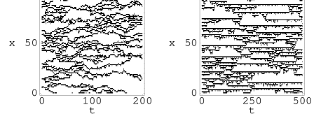
Figure 3: Equilibrium space-time trajectories at $T=1.0$ for the $1+1$-dimensional FA (left) and East (right) models, reproduced from Garrahan-Chandler . Up-spins are black, down spins white. Space runs along the vertical direction, encompassing $10^{5}$ spins. Time runs along the horizontal. The characteristic length scales of both systems correspond to the vertical extent of the ‘bubbles’ of down-spins, which scale in equilibrium as $l_{eq}\sim c^{-1}$. The horizontal extent, $\tau$, of the bubbles is determined by the relation $\tau\sim l^{z}$, where the dynamical exponents for the FA and East models are $z=2$ and $z\propto 1/T$, respectively. As one observes the trajectories shown above on smaller length and shorter time scales, one moves from right to left along the RG flow diagrams shown in Figures 4 and 1. Hence one eventually probes behaviour controlled by the critical fixed point. For the East model, the disappearance of the characteristic length is consistent with the emergence of the fractal structure of the bubble boundaries.

VI Renormalization of the East model

The East model is defined by Equation (15). To renormalize it using a blocking parameter $p=2$, for example, we need only consider the $16\times 16$ matrix

$$\mathcal{H}^{E}=(n\otimes\ell)\otimes(1\otimes 1)+(1\otimes n)\otimes(\ell\otimes 1).$$ (43)

The brackets indicate the groupings of cells into blocks. The first term in (43) is the intra-cell component $\mathcal{H}_{0}$; the second is the inter-cell interaction $V_{\alpha,\alpha+1}$.

We must calculate the left and right ground states of the matrix $\mathcal{H}_{0}$ (15). The left ground states are represented by the row vectors $(0,0,0,1),(0,0,1,0)$ and $(1,1,0,0)$. The right ground states correspond to the column vectors $(0,0,0,1)^{T},(0,0,1,0)^{T}$ and $[c/(1-c),1,0,0]^{T}$. Next, we choose the projection and embedding matrices, which we call $R_{1}$ and $R_{2}$ so as not to confuse them with their FA model counterparts. One choice satisfying criteria 1–4 (see above) is

$$R_{1}=\left(\begin{array}[]{cccc}1&1&1&0\\ 0&0&0&1\end{array}\right),\quad R_{2}=\left(\begin{array}[]{cc}ac&0\\ a(1-c)&0\\ 1-a&0\\ 0&1\end{array}\right),$$ (44)

where $0<a<1$ parameterizes a degree of freedom. This arises because the East model admits one more ground state vector than the FA model. $R_{1}$ projects $\left|\uparrow\uparrow\right\rangle,\left|\uparrow\downarrow\right\rangle$ and $\left|\downarrow\uparrow\right\rangle$ onto $\left|+\right\rangle$, and $\left|\downarrow\downarrow\right\rangle$ onto $\left|-\right\rangle$. $R_{2}$ embeds the state $\left|+\right\rangle$ as $ac\left|\uparrow\uparrow\right\rangle+a(1-c)\left|\uparrow\downarrow\right\rangle+(1-a)\left|\downarrow\uparrow\right\rangle$, and $\left|-\right\rangle$ as $\left|\downarrow\downarrow\right\rangle$. With this choice we get

$$(\mathcal{H}^{E})^{\prime}=(1+ac-a)\left(\begin{array}[]{cccc}a(1-c)^{2}&-c&0&0\\ -a(1-c)^{2}&c&0&0\\ 0&0&0&0\\ 0&0&0&0\end{array}\right).$$ (45)

We deduce the flow of the temperature parameter in a similar way to before: let the ratio of the rates of the processes $A\emptyset\rightarrow AA$ and $AA\rightarrow A\emptyset$ be $\lambda$. Then

$$\lambda_{0}\equiv-\frac{(1,2)}{(1,1)}=\frac{c}{1-c}=e^{-1/T}$$ (46)

where $(i,j)$ is element $(i,j)$ of matrix (15). Hence the bare temperature parameter has the same interpretation as in the FA model. We can work out how $\lambda$ renormalizes by calculating the ratio of elements $(1,2)$ and $(1,1)$ of matrix (45). The resulting RG recursion relation is

$$\lambda^{\prime}=a^{-1}\lambda(1+\lambda),$$ (47)

implying an unstable zero-temperature critical point, $\lambda^{\star}=0$, as expected.

The dynamical exponent $z$ follows immediately. In the critical limit $\lambda\rightarrow 0$, element $(1,1)$ of matrix (15) becomes unity. Hence we may interpret the renormalized value of this element as the time rescaling factor $2^{-z}$. From (45) we get

$$2^{-z}=\lim_{c\rightarrow 0}\Big{\{}1+a(c-1)\Big{\}}a,$$ (48)

and so $z$ depends on the value we choose for $a$.

Let us choose $a$. This parameter measures the extent to which we treat the states $\left|\downarrow\uparrow\right\rangle$ and $\left|\uparrow\downarrow\right\rangle$ on equal footing. In a model with symmetric dynamical rules, such as the FA model, we must treat these states identically. But the East model has asymmetric dynamical rules, suggesting that at some point in our calculation we must suppress $\left|\downarrow\uparrow\right\rangle$ relative to $\left|\uparrow\downarrow\right\rangle$, or vice-versa. At which point should we do this? We note that the projection matrix $R_{1}$ treats $\left|\uparrow\downarrow\right\rangle$ and $\left|\downarrow\uparrow\right\rangle$ identically. If this were not the case, and we instead (for example) used

$$R^{\prime}_{1}=\left(\begin{array}[]{cccc}1&1&0&0\\ 0&0&1&1\end{array}\right),$$ (49)

we would violate criteria 2 and 3 above. ($R^{\prime}_{1}$ imposes a symmetry between flipping spins $\uparrow\leftrightarrow\downarrow$ in a two-spin block and flipping the resulting renormalized spin $\left|+\right\rangle\leftrightarrow\left|-\right\rangle$.) Therefore, we conclude that the embedding matrix $T_{2}$ must treat $\left|\uparrow\downarrow\right\rangle$ and $\left|\downarrow\uparrow\right\rangle$ asymmetrically. The simplest way of doing this is to set $a=1$, thus suppressing completely the state $\left|\downarrow\uparrow\right\rangle$. This corresponds to the assertion that a spin configuration $\left|\downarrow\uparrow\right\rangle$ (which is unable to change state unless connected to neighbouring spins) is much less important to the dynamics than a configuration $\left|\uparrow\downarrow\right\rangle$, which is mobile. Thus when one renormalizes the lattice using $R_{1}$ and $R_{2}$ with $a=1$, one effectively discards dynamical pathways mediated by blocks of ‘jammed’ spins $\left|\downarrow\uparrow\right\rangle$. The RG process discards inaccessible pathways in trajectory space $\{\sigma_{t_{1}},\sigma_{t_{2}},\dots\}$, according to rules imposed by the Liouvillian of the dynamical process. Loosely, the projection matrix $R_{1}$ identifies those single-spin states which are facilitating, whereas $R_{2}$ picks out those two-spin states which are (internally) mobile.

Setting $a=1$ immediately yields a temperature dependent dynamic exponent: from Equation (48) we obtain $2^{-z}=c$, or $z=(T\ln 2)^{-1}$. Were $a<1$, $z$ would be independent of temperature to leading order. We thus conclude that maximal spatial anisotropy in the embedding process is a necessary condition for a temperature-dependent dynamic exponent.

The RG scheme for the East model can be generalized to larger block sizes. However, this procedure is less straightforward than for the FA model, because of the freedom one is afforded by the East model’s many ground state eigenvectors. Furthermore, the results one obtains depends on whether one coarse-grains using a blocking parameter $p$ equal to a power of $2$, or not.

Let us first illustrate the generalization of the procedure for the case $p=4=2^{2}$. We show that the results are consistent with the $p=2$ scheme. We then argue that one should obtain a different dynamical exponent if one coarse-grains the system using a block size not equal to a power of $2$, and then show explicitly for $p=3$ that this is indeed the case.

Consider $p=2^{n}$, where $n$ is an integer. Building $R_{1}^{(p)}$ is straightforward: it is identical to $T_{1}^{(p)}$, its FA model counterpart. Thus $R_{1}^{(4)}$ is a $2\times 16$ matrix whose top row is composed of $1$s apart from the rightmost element which is zero. Vice versa for the bottom row.

The form of the embedding matrix is less obvious, because the number of ground states increases as one increases the block size. However, we are guided by the form of the Liouvillian, which for block size $p=4$ may be written schematically as

$$\mathcal{H}^{E} = (n\otimes\ell\otimes 1\otimes 1)+(1\otimes 1\otimes n\otimes\ell)$$

$$+ \qquad\qquad(1\otimes n\otimes\ell\otimes 1)$$

$$+ (\ell\otimes 1\otimes 1\otimes 1)+(1\otimes 1\otimes 1\otimes n).$$

Brackets again denote the grouping of cells into blocks. We take the first line of Equation (VI) as the intra-cell Hamiltonian $\mathcal{H}_{0}$. The second line vanishes under renormalization as a consequence of $T_{1}$ acting on it from the left, and so we ignore it; the third line comprises the inter-cell interaction whose renormalization properties we wish to study.

Guided by the form of $R_{2}^{(2)}$, we find that one choice of $R_{2}^{(4)}$ satisfying criteria 1–4 above is

$$R_{2}^{(4)}=\mathcal{N}^{(4)}(\lambda)\left(\begin{array}[]{cc}\lambda^{3}&0\\ \lambda^{2}&0\\ 0&0\\ \lambda&0\\ \lambda^{2}&0\\ \lambda&0\\ 0&0\\ 1&0\\ 0&0\\ 0&0\\ 0&0\\ 0&0\\ 0&0\\ 0&0\\ 0&0\\ 0&\mathcal{N}^{(4)}(\lambda)^{-1}\end{array}\right),$$ (51)

where $\mathcal{N}^{(4)}=\left(1+2\lambda+2\lambda^{2}+\lambda^{3}\right)^{-1}$. We see that Equation (51) can be obtained from its FA model counterpart by using a simple rule-of-thumb: suppress all states of the form $\left|\downarrow\cdots\right\rangle$ [corresponding to elements $(9,1)$–$(18,1)$ of (51)], as well as states possessing a ‘frozen’ up-spin at the right-hand boundary of the block. Thus states $\left|\uparrow\uparrow\downarrow\uparrow\right\rangle$ [corresponding to element $(3,1)$ of (51)] and $\left|\uparrow\downarrow\downarrow\uparrow\right\rangle$ [element $(7,1)$] have been removed. We see again that the embedding operator plays the role of a dynamical ‘filter’, eliminating those states which play a sub-dominant role in the dynamics of the East model.

With these choices of embedding and projection operators we obtain the RG recursion relation for the temperature,

$$\lambda_{(4)}^{\prime}=\lambda\left(1+2\lambda+2\lambda^{2}+\lambda^{3}\right),$$ (52)

and a relation for the dynamical exponent:

$$4^{-z}=\lim_{\lambda\to 0}\frac{\lambda^{2}(1+\lambda)}{\left(1+\lambda+\lambda^{2}\right)^{2}}.$$ (53)

Equation (52) is identical to the result one would obtain via two coarse-grainings using a block size $p=2$ [Equation (47)], as required. Equation (53) yields the dynamical exponent $z=\left(T\ln 2\right)^{-1}$, as before.

We shall demonstrate how one can generalize this approach to arbitrarily large $n$. Let us use reaction-diffusion notation $(\uparrow\to 1,\downarrow\to 0$), and write the projection and embedding operators in the form

$$\hat{R}_{1}=\left|+\right\rangle\left(\sum_{1\star}\left\langle 1\star\right|\right)+\left|-\right\rangle\left\langle 00\cdots 0\right|,$$ (54)

and

$$\hat{R}_{2}=\left(\sum_{1\star}a_{1\star}\left|1\star\right\rangle\right)\left\langle+\right|+\left|00\cdots 0\right\rangle\left\langle-\right|.$$ (55)

The symbol $1\star$ denotes any state $\left|1\cdots\right\rangle$ starting with a $1$, and the $\{a_{1\star}\}$ are a set of coefficients [see e.g. the first column of (51)]; the projection operator $\hat{R}_{1}$ allows one to compare this notation to the matrix representations employed previously. The normalization requirement $\hat{R}_{1}\cdot\hat{R}_{2}=\mathbf{1}$ implies $\sum_{1\star}a_{1\star}=1$. Thus at least one of the coefficients $a$ must be of $\mathcal{O}(1)$.

The values of these coefficients are fixed by the eigenvectors of the intra-block evolution operator, as we have discussed. We can see how these coefficients determine the properties of the model under renormalization, as follows. We find that ‘bulk’ states of the form $(\cdots 1\otimes\hat{n}\otimes\hat{\ell}\otimes 1\cdots)$ vanish under renormalization as a consequence of the projection operator acting from the left. We are therefore left with the ‘surface’ terms $(\hat{\ell}\otimes 1\otimes\cdots\otimes 1)$ and $(1\otimes\cdots\otimes\hat{n})$, in which the operators $\hat{n}$ and $\hat{\ell}$ sit at the edge of the block. We find that, under renormalization,

$$\hat{R}_{1}\cdot\left(1\otimes\cdots\otimes\hat{n}\right)\cdot\hat{R}_{2}\to\left(\sum_{1\star 1}a_{1\star 1}\right)\hat{n}^{\prime}$$ (56)

and

$$\hat{R}_{1}\cdot\left(\hat{\ell}\otimes 1\otimes\cdots\otimes 1\right)\cdot\hat{R}_{2}\to\left(a_{10\cdots 0}\right)\,\hat{\ell}^{\prime}\left[\lambda\to\frac{\lambda}{a_{10\cdots 0}}\right].$$ (57)

In Equations (56) and (57) primes denote renormalized operators. The symbol $1\star 1$ denotes states $\left|1\cdots 1\right\rangle$ starting and ending with a $1$. In (57) the temperature parameter $\lambda$ has been rescaled by the coefficient $a_{10\cdots 0}$ which weights thermally the state $\left|10\cdots 0\right\rangle$ with a single $1$ at the leftmost edge, followed by a string of $0$s. From the previous discussion we know that this coefficient is of order unity, and hence the recursion relation for $\lambda$ will be marginal, as we have found.

The dynamical exponent follows by noting that the product of Equations (56) and (57) constitutes the renormalized evolution operator, and so the prefactor describes the rescaling of time as a consequence of rescaling space. Thus

$$p^{-z}\propto\lim_{\lambda\to 0}\left(a_{10\cdots 0}\right)\times\left(\sum_{1\star 1}a_{1\star 1}\right).$$ (58)

The constant of proportionality in (58) is $(1-c)^{-1}=1+\lambda$, i.e. the reciprocal of element $(1,1)$ in the unrenormalized East model Hamiltonian (15). The first factor on the right hand side of (58) is of order unity. The second factor is fixed by the embedding operator, which is in turn determined by the relevant East model eigenvectors. The rule-of-thumb we obtained above tells us that we remove from this factor any state with a frozen rightmost up-spin. This may be regarded as an entropic suppression of states playing only a sub-dominant role in the dynamics. Those states starting and ending with a 1 which are important for the dynamics of the East model are for block sizes $p=2,4,8$ and $16$,

$$11\left(\lambda\right),1011\left(\lambda^{2}\right),10001011\left(\lambda^{3}\right),$$

$$1000000010001011\left(\lambda^{4}\right).$$ (59)

All have a ‘mobile’ rightmost up-spin. The thermal weighting of each state is given in brackets. These states are important because of the hierarchical dynamics of the East model Ritort-Sollich ; Sollich-Evans , which dictates that two defects separated by a distance $d$ are relaxed by establishing a set of isolated defects between them, at distances $d/2$, $3d/4$ etc. Thus for block size $p=4$ the dominant dynamical pathway proceeds via the state $1011$, with a thermal weighting of $\lambda^{2}$ (and not, for example, $1001$, which has a weighting of $\lambda$). Hence $a_{1011}\sim\lambda^{2}$, $a_{1001}=0$, and so $\lim_{\lambda\to 0}\sum_{1\star 1}a_{1\star 1}\sim\lambda^{2}$. Consequently, the rescaling factor is $4^{-z}\sim\lambda^{2}$, and the dynamical exponent $z=(T\ln 2)^{-1}$, as required. (In the FA model, states such as $\left|0001\right\rangle$ are permitted, leading to temperature-independent $a$ coefficients and hence to a temperature-independent $z$.) Thus $R_{2}$, which attempts to reconstitute an unrenormalized state from a coarse-grained state, captures both energetic effects (the powers of $\lambda$ weighting thermally the various states) and entropic effects (the ‘zero’ entries corresponding to those suppressed entropically). We conclude that the RG scheme for the East model generalizes readily to larger block sizes.

It is interesting to note that if one uses blocks of size not equal to a power of $2$, one obtains a slightly different result for the dynamical exponent. We argue that this is a consequence of the hierarchical dynamics of the East model taking place naturally in blocks of lengths equal to a power of $2$ Ritort-Sollich ; Sollich-Evans . We can derive the approximate value of $z$ that one should obtain from a coarse-graining over block sizes $p\neq 2^{n}$. Let us take $p=3$ as an illustration. Consider the coarse-grained relaxation process $\left|++\right\rangle\stackrel{{\scriptstyle\gamma^{\prime}}}{{\longrightarrow}}\left|+-\right\rangle$. We wish to determine the leading order temperature dependence of $\gamma^{\prime}$, noting that the rate for the equivalent unrenormalized process, $\left|\uparrow\uparrow\right\rangle\stackrel{{\scriptstyle\gamma_{0}}}{{\longrightarrow}}\left|\uparrow\downarrow\right\rangle$, is $\gamma_{0}=\mathcal{O}(1)$. From our previous discussion of the form of the embedding matrices, we can infer that the dominant dynamical pathway (involving ‘unrenormalized’ spins) contributing to this renormalized process is $\left|\uparrow\downarrow\downarrow\uparrow\downarrow\downarrow\right\rangle\stackrel{{\scriptstyle\gamma_{1}}}{{\longrightarrow}}\left|\uparrow\downarrow\downarrow\downarrow\downarrow\downarrow\right\rangle$. To relax the second up-spin, one must create two extra up-spins to the right of the first up-spin. Hence this pathway has a rate $\gamma_{1}\sim c^{2}$, and the renormalized rate $\gamma^{\prime}=\mathcal{O}(c^{2})$. Other pathways also contribute to the renormalized process $\left|++\right\rangle\stackrel{{\scriptstyle\gamma^{\prime}}}{{\longrightarrow}}\left|+-\right\rangle$, but do so either with rates $\sim c^{2}$ (e.g. $\left|\uparrow\uparrow\downarrow\uparrow\downarrow\downarrow\right\rangle\longrightarrow\left|\uparrow\downarrow\downarrow\downarrow\downarrow\downarrow\right\rangle$)—in which case $\gamma^{\prime}$ is changed only by a temperature-independent numerical factor—or with rates higher order in $c$ (e.g. the pathway $\left|\uparrow\uparrow\uparrow\uparrow\downarrow\uparrow\right\rangle\longrightarrow\left|\uparrow\downarrow\uparrow\downarrow\downarrow\downarrow\right\rangle$). These we may ignore. Since we interpret the overall rescaling of the fundamental relaxation rate deriving from a coarse-graining of space as the numerical factor $p^{-z}$, we would therefore expect for $p=3$ that $3^{-z}\sim c^{2}$, or $z\sim 2/(T\ln 3)$.

Loosely, then, we expect that by coarse-graining space in blocks of size $2^{n-1}<p<2^{n}$ one should obtain $z\approx n/\left(T\ln p\right)$ [which tends to $z\to(T\ln 2)^{-1}$ when $p\to\infty$]. Coarse-graining using block sizes $p=2^{n}$ yields $z=(T\ln 2)^{-1}$. This is as we expect: the energetic barriers for relaxing chains of lengths $2^{n-1}<p<2^{n}$ and $p=2^{n}$ are identical, but the entropic barriers are larger for the latter case. Thus one would expect the dynamical exponents to differ. More sophisticated arguments Aldous-Diaconis reveal that $z$ is bounded by $(T\ln 2)^{-1}$ and $(2T\ln 2)^{-1}$.

We can show that our guess for the dynamical exponent is borne out in the case $p=3$ by the RG scheme. We construct the embedding operator according to the

$$R_{2}^{(3)}=\mathcal{N}^{(3)}(\lambda)\left(\begin{array}[]{cc}\lambda^{2}&0\\ \lambda&0\\ 0&0\\ 1&0\\ 0&0\\ 0&0\\ 0&0\\ 0&\mathcal{N}^{(3)}(\lambda)^{-1}\end{array}\right),$$ (60)

where $\mathcal{N}^{(3)}=\left(1+\lambda+\lambda^{2}\right)^{-1}$. Together with the obvious choice for the projection operator we find

$$3^{-z}=\lim_{\lambda\to 0}\frac{\lambda^{2}}{\left(1+\lambda+\lambda^{2}\right)^{2}},$$ (61)

yielding $z=2/\left(T\ln 3\right)$, as advertised. We conclude that the RG scheme for the East model can be generalized to larger block sizes, but more naturally so for the case of a blocking parameter $p$ equal to a power of $2$. For simplicity we shall focus on the case $p=2$.

With $a=1$ the RG recursion relation (47) may be iterated to give

$$\lambda_{p}=\lambda_{0}+n\lambda_{0}^{2}+\mathcal{O}\left(\lambda^{3}\right).$$ (62)

where $\lambda_{p}$ is the value of the temperature parameter following a coarse-graining of the system by a factor $p=2^{n}$. Since the bare value of $\lambda_{0}>0$, we see that (62) describes a system with an unstable zero-temperature critical point $\lambda^{\star}=0$, and a stable high-temperature fixed point $\lambda^{\star}\rightarrow\infty$. Now, however, the temperature parameter $\lambda$ is marginally relevant near the fixed point $\lambda^{\star}=0$. The RG flow diagram is shown in Figure 4.

Figure 4: East model RG flow diagram for the temperature paramter $c=(1+e^{1/T})^{-1}$. The zero-temperature critical fixed point $c^{\star}=0$ $(\lambda^{\star}=0)$ is unstable. Near this fixed point, corresponding to observations of the system on small length and time scales, the East model admits no characteristic length. This is consistent with the fractal structure of space-time trajectories seen in numerical simulations, such as those shown in Figure 3. The dynamical exponent $z$ is proportional to $1/T$, indicating a rapid slowing-down of the dynamics near the critical point. As one observes the system on progressively larger length and time scales, one sees the emergence of a characteristic length growing as the double exponential of reciprocal temperature. This length saturates rapidly, and is eventually supplanted as the characteristic length of the system by by the equilibrium domain size, whose properties are controlled by the high-temperature stable fixed point $c^{\star}=1$ $(\lambda^{\star}=\infty)$.

To determine the correlation length in the East model we proceed as follows. From the recursion relation (62) we see that the correlation length satisfies

$$\xi\left(x+\frac{\ln p}{\ln 2}~{}x^{2}\right)=p^{-1}\xi(x).$$ (63)

For small values of $x=\lambda$, corresponding to low temperatures, we have no solution $\xi(\lambda)$ of (63) to first order in $\lambda$. Thus near criticality the East model possesses no characteristic length scale. This is consistent with the nature of the space-time trajectories seen in numerical simulations, such as that shown in the right panel of Figure 3. These display a fractal structure Garrahan-Chandler , and hence possess no characteristic length.

On sufficiently large length and time scales the system will reach equilibrium, at which point the heights of bubbles will be determined by the equilibrium spin distribution. This does have a characteristic length. One therefore expects to see, sufficiently far from criticality, the emergence of a length scale. Below, we show that Equation (63) indeed admits a growing length in such a regime. This corresponds to the eventual ‘blurring out’ of the fractal boundaries of clusters as one observes the system on progressively larger scales. The emerging length scale corresponds to the spatial extent of bubble regions.

We can quantify the emergence of this length by considering an infinitesimal RG transformation. The blocking parameter $p$ is necessarily an integer, because our model is defined on a lattice. But we can generalize $p$ by considering an infinitesimal change of scale according to $p=1+\ell$, where $\ell\ll 1$. By writing $\xi(\lambda+\ell\lambda^{2}/\ln 2)\approx\xi(\lambda)+\ell d\xi(\lambda)/d\ell$ and $\lambda^{\prime}-\lambda\approx\ell d\lambda/d\ell$ we obtain the flow equations for the temperature and correlation length:

$$\frac{d\lambda(\ell)}{d\ell}=\lambda(\ell)^{2}/\ln 2,$$ (64)

and

$$\frac{d\xi(\ell)}{d\ell}=-\xi(\ell).$$ (65)

The intial data for Equations (64) and (65) are $\lambda(\ell_{0})=\lambda_{0}$ and $\xi(\ell_{0})=\xi_{0}$, respectively, where the subscript zero denotes an unrenormalized (physically meaningful) quantity. The parameter $\ell_{0}$ acts as a short distance regulator (or ultraviolet cutoff), and should be taken to zero at the end of the calculation.

One now iterates the RG by integrating (64) until $\lambda(\ell)=\mathcal{O}(1)$, yielding $\ell-\ell_{0}\approx\ln 2/\lambda_{0}$. From (65) we obtain $\xi(\ell)=\xi_{0}e^{-(\ell-\ell_{0})}$, and so the correlation length varies with temperature according to

$$\xi_{0}(\lambda_{0})\sim\exp\left(1/(\lambda_{0}\ln 2)\right)\sim\exp\left(e^{1/T}/\ln 2\right).$$ (66)

Away from the critical point $\lambda^{\star}=0$ we therefore see an extremely rapid growth of the dynamical length scale with temperature.

This length scale corresponds to the emergence of a characteristic length $\xi_{d}$ away from criticality, and not to an equilibrium length scale $l_{eq}$. The latter may be defined as the reciprocal of the particle density in the steady state (see below), and scales as $c^{-1}$. The dynamical length is a nonequilibrium critical quantity, and will be cut off rapidly as one probes larger length and time scales. Thus, in terms of the RG flow diagram, Figure 4, the steady-state behaviour is obtained near the attractive fixed point $\lambda^{\star}\rightarrow\infty$, where one probes length and time scales much larger than those on which critical fluctuations are manifest. The critical behaviour will be observed on short length and time scales, near the critical fixed point $\lambda^{\star}=0$.

The characteristic equilibration time follows from the relation $\tau\sim l^{z}$, where $l$ is a typical length scale. We have $z=(T\ln 2)^{-1}$. Taking the equilibrium domain length $l_{eq}\sim\lambda^{-1}$, we find the equilibration time scale $\tau_{eq}\sim c^{-z}\sim\lambda^{\ln\lambda}=\exp\{1/(T^{2}\ln 2)\}$. This agrees with results obtained by other means Ritort-Sollich . We assume that the dynamical exponent $z$ obtained near criticality holds in the region of the attractive fixed point.

One may also calculate Hooyberghs the density of particles, $n=\frac{1}{2}(1+\sigma)$. First note that the number operator renormalizes differently depending on whether $n$ sits in the left or right slot of the block: $(n\otimes 1)^{\prime}=n_{\alpha}$, versus $(1\otimes n)^{\prime}=cn_{\alpha}$. Hence we will define our density operator as $n=\frac{1}{2}(n\otimes 1+1\otimes n)$. The RG recursion relation for the density then reads

$$n_{k}=\frac{1}{2}\left(\frac{1+2\lambda_{k}}{1+\lambda_{k}}\right)n_{k+1}.$$ (67)

To extract the steady-state density we write (67) as $n(\lambda_{k})=a(\lambda_{k})n(\lambda_{k+1})$, where $a(x)=(1+2x)/\left[2(1+x)\right]$. By iterating this equation along the RG flow we get

$$n_{s}(\lambda_{0})=\left[\prod_{i=0}^{\infty}a(\lambda_{i})\right]n(\lambda^{\star}_{a}),$$ (68)

where $n_{s}$ is the steady-state density, and $n(\lambda^{\star}_{a})$ is the density at the attractive fixed point $\lambda^{\star}_{a}=\infty$. Next, define $G_{n}(\lambda)\equiv\prod_{i=0}^{n}a(\lambda_{i})$. From Equations (62) and (67) we can write

$$a(\lambda_{k})=\frac{1}{2}\frac{d\ln\lambda_{k+1}}{d\ln\lambda_{k}},$$ (69)

as in the FA model. Hence

$$G_{n}(\lambda)=\frac{\lambda_{0}}{\lambda_{0}+1}\left(1+\mathcal{O}(\lambda_{n+1}^{-1})\right).$$ (70)

Taking $n\rightarrow\infty$ gives $\lambda_{n+1}\rightarrow\infty$, and by noting that $n(\lambda^{\star}_{a})=1$ we obtain the steady-state density

$$n_{s}(\lambda_{0})=\frac{\lambda_{0}}{\lambda_{0}+1}=c,$$ (71)

as expected.

The behaviour of the density near criticality ($\lambda^{\star}=0$) follows from the relation $n(\Delta\lambda)=a(\lambda^{\star})n(\lambda^{\prime})$, where $\Delta\lambda\equiv\lambda-\lambda^{\star}=\lambda$. If we iterate the RG until the renormalized coupling $\lambda^{\prime}=\mathcal{O}(1)$, i.e. $\ell/\ell_{0}\sim e^{\ln 2/\lambda_{0}}$, we find $n(\lambda_{0})\sim e^{-\ln 2/\lambda_{0}}$. Thus the density vanishes close to the critical point faster than any power of $T$.

VII Renormalization of the BCIC

In this section we will apply the RG scheme to the BCIC, a model whose kinetic constraint interpolates between that of the East and FA models. We find that on suitably large length and time scales (or for suitably low temperatures) the BCIC behaves like the FA model. This agrees with existing numerical and analytical results Buhot-Garrahan .

The ground state eigenvectors of the BCIC (14) are the same as those of the FA model. If we use (28) and (14) we find

$$(\mathcal{H}^{b})^{\prime}=\frac{1}{2-c}\left(\begin{array}[]{cccc}\frac{1}{2-c}-c&-\tilde{b}c&-bc&0\\ \frac{\tilde{b}}{c-2}+\tilde{b}c&\tilde{b}c&0&0\\ \frac{b}{(c-2)}+bc&0&bc&0\\ 0&0&0&0\end{array}\right).$$ (72)

Equations (14) and (72) yield the same recursion relation for the temperature parameter $\lambda$ as in the FA model, $\lambda_{k+1}=\lambda_{k}(2+\lambda_{k})$. They also yield a recursion relation for the asymmetery parameter $b$: $b_{k+1}=b_{k}$. Thus the asymmetry $b$ is a marginal operator, and does not flow under renormalization. From the RG relation for $\lambda$, we see that for any $b\in(0,1)$ the interpolation model falls in the universality class of the FA model, rather than the East model.

However, we expect the interpolation model for small values of $b$ to display a crossover from East-like to FA-like behaviour Buhot-Garrahan . This suggests that by projecting $\mathcal{H}^{b}$ onto a subspace spanned by only the ground states of (14) we have omitted this crossover behaviour. We can recover it in the following way.

First, we note that the difference between the East and FA models manifests itself in the treatment of the states $\left|\uparrow\downarrow\right\rangle$ and $\left|\downarrow\uparrow\right\rangle$ during embedding. In the East model the latter is completely suppressed (see Equation (44)); in the FA model, both are treated on equal footing [Eq. (28)]. By restricting our RG scheme to a subspace of the ground states of Equation (14), we are unable to construct an embedding operator that treats $\left|\downarrow\uparrow\right\rangle$ and $\left|\uparrow\downarrow\right\rangle$ asymmetrically [cf. $R_{2}$, Equation (44)].

To remedy this, we now include the first excited right eigenvector of (14) in our embedding operator. We will call this eigenvector $e$. This is akin to calculating higher-order “loop” diagrams to check if $b$, ostensibly a marginal operator, is relevant at second order. $e$ has eigenvalue $2(1-b)bc+\mathcal{O}(c^{2})$, and is therefore a “gapless excitation” in the East model limit, $b\rightarrow 0$. Note that $e=(e_{1},e_{2},1,0)^{T}$, where the $e_{i}$ are functions of $c$ and $b$. For small $c$ we have $e\approx\left[(2b-1)c,-1+(1-2b)c,1,0\right]$.

Let us now construct a new embedding operator,

$$\tilde{R}_{2}=\frac{1}{2-c}\left(\begin{array}[]{cc}c+\alpha e_{1}&0\\ 1-c+\alpha e_{2}&0\\ 1-c+\alpha&0\\ 0&2-c\end{array}\right),$$ (73)

and demand that in the limits $b\rightarrow 0$ and $b\rightarrow\frac{1}{2}$ we recover the respective embedding operators for the East and FA models, namely $R_{2}$ and $T_{2}$. This is achieved by setting $\alpha=-(1-2b)(1-c)$. We note that $R_{1}\tilde{R}_{2}=\mathbf{1}$.

Our renormalization prescription is now $(\mathcal{H}^{b})^{\prime}=R_{1}\mathcal{H}^{b}\tilde{R}_{2}$. We derive recursion relations for the parameters $c$ and $b$ in a similar way to before: we define the unrenormalized temperature parameter $\lambda$ as the ratio

$$\lambda\equiv-\frac{(1,2)+(1,3)}{(1,1)}=\frac{c}{1-c},$$ (74)

where $(i,j)$ is element $(i,j)$ of the matrix $\mathcal{H}_{b}\equiv\mathcal{L}$, Equation (14). We define the renormalized parameter $\lambda^{\prime}$ by the ratio of the corresponding elements of the renormalized matrix $(\mathcal{H}^{b})^{\prime}$. This gives us the recursion relation $\lambda_{k+1}=f(\lambda_{k},\mu_{k})$. The parameter $\mu$ is the scaled asymmetry parameter, whose unrenormalized value we define as

$$\mu\equiv\frac{(1,3)}{(1,2)}=\frac{b}{1-b}.$$ (75)

The elements $(i,j)$ again refer to Equation (14). We write the recursion relation for $\mu$, obtained from the elements of $(\mathcal{H}^{b})^{\prime}$, as $\mu_{k+1}=g(\lambda_{k},\mu_{k})$.

The behaviour of the functions $f$ and $g$ thus determine the crossover properties of our model. We find that $\lambda$ has an unstable zero-temperature fixed point $\lambda^{\star}=0$, and an attractive high-temperature fixed point $\lambda^{\star}\rightarrow\infty$. The asymmetry $\mu$ has an unstable maximal-aysymmetry fixed point $\mu^{\star}=0$, corresponding to the East model, and an attractive symmetric fixed point $\mu^{\star}=1$, corresponding to the FA model. Thus any BCIC with less than maximal asymmetry will behave at long length and time scales like the FA model. Figure 5 shows the qualitative RG flow of the BCIC.

For the case of $p=2$ we find that

$$\lambda_{k+1}=\left\{\begin{array}[]{lr}\lambda_{k}(1+\lambda_{k})+f_{1}(\lambda_{k})\mu_{k}+\mathcal{O}(\mu_{k}^{2}),&\mu_{k}\approx 0;\\ \lambda_{k}(2+\lambda_{k})+f_{2}(\lambda_{k})\tilde{\mu}_{k}^{2}+\mathcal{O}\left(\tilde{\mu}_{k}^{3}\right),&\mu_{k}\approx 1,\end{array}\right.$$ (76)

where $f_{1}(x)\equiv(2+9x+11x^{2}+6x^{3}+x^{4})(2+3x+x^{2})^{-1}$, $f_{2}(x)\equiv x^{2}(x-1)(2+x)/[8(1+x)]$, and $\tilde{\mu}_{k}\equiv 1-\mu_{k}$. Equations (76) thus reproduce the recursion relations for $\lambda$ in the East model and FA model limits, respectively Equations (47) and (31). The asymmetry parameter $\mu$ is a relevant perturbation, whose flow is governed by

$$\mu_{k+1}=\left\{\begin{array}[]{lr}\left(1+\frac{1}{\lambda_{k}}\right)\mu_{k}-f_{3}(\lambda_{k})\mu_{k}^{2}+\mathcal{O}(\mu_{k}^{3}),&\mu_{k}\approx 0;\\ 1-\frac{\lambda_{k}}{1+\lambda_{k}}\tilde{\mu}_{k}+\mathcal{O}\left(\tilde{\mu}_{k}^{2}\right),&\mu_{k}\approx 1,\end{array}\right.$$ (77)

where $f_{3}(x)\equiv(2+4x+5x^{2}+3x^{3})/[x^{2}(1+x)(2+x)]$.

We can deduce the flow of the BCIC away from maximal asymmetry, $\mu=0$, by studying Equations (76) and (77) in the regime $\mu\ll\lambda\ll 1$. Writing $\beta_{\lambda}\equiv\lambda^{\prime}-\lambda\approx\ell d\lambda/d\ell$, and a similar relation for $\mu$, we obtain

$$\beta_{\lambda} = \ell\lambda^{2}+\mu+\mathcal{O}(\lambda\mu)+\mathcal{O}(\mu^{2}/\lambda);$$ (78)

$$\beta_{\mu} = \frac{\mu}{\lambda}-\frac{\mu^{2}}{\lambda^{2}}+\mathcal{O}(\mu^{3}/\lambda^{3})+\mathcal{O}(\mu^{2}/\lambda).$$ (79)

Equations (78) and (79) may be solved in terms of the exponential integral function $Ei\left(\lambda^{-1}\right)$, although the physical interpretation of this solution is not obvious. We can more clearly determine the essence of the crossover as follows.

The temperature parameter $\lambda$ has RG eigenvalue 0 (East model) or 1 (FA model). It therefore grows much less rapidly than the asymmetry parameter $\mu$, which has (initial) eigenvalue $\lambda_{0}^{-1}\gg 1$. Hence from (77) we have $\mu^{\prime}=2^{y_{\mu}}\mu\approx\lambda_{0}^{-1}\mu$, giving the RG eigenvalue for the asymmetry parameter as $y_{\mu}\approx\left(T\ln 2\right)^{-1}$. Let us now write a standard RG scaling form for the particle density,

$$n_{R}(\lambda^{\prime},\mu^{\prime})=p\,n\left(p^{y_{\lambda}}\lambda,p^{y_{\mu}}\mu,p^{-1}\xi,p^{-z}t\right)$$ (80)

To derive a crossover temperature, we iterate the RG until $p^{y_{\lambda}}=\mathcal{O}(1)$. The $\mu-$dependent scaling combination is then $\lambda^{-y_{\mu}/y_{\lambda}}$. When this becomes large, i.e. $\mathcal{O}(1)$, one would expect the BCIC to behave like the FA model. Taking for simplicity $y_{\lambda}=1$, we find a crossover temperature $T_{xo}\sim\left(-\ln\mu\right)^{-1/2}$. This scaling agrees with that obtained by equating the relaxation timescale for the $\mu$-suppressed symmetric process, $\tau_{S}\sim\left(\mu\lambda\right)^{-1}$ with that for the asymmetric process, $\tau_{A}\sim\exp\left(1/T^{2}\ln 2\right)$ Buhot-Garrahan ; Garrahan-Chandler .

We can extract crossover time- and length-scales from Equation (80) by iterating the RG until, respectively, $p^{-1}\xi=\mathcal{O}(1)$ and $p^{-z}t=\mathcal{O}(1)$. These give $\xi_{xo}\sim\mu^{-T\ln 2}$ and $t_{xo}\sim\mu^{-2T\ln 2}$.

Figure 5: RG flow diagram for the BCIC, in $(\lambda,\mu)$ space. $\mu=0$ (resp. 1) corresponds to East (resp. FA) model behaviour. The critical fixed point $(0,0)$ is unstable; the attractive fixed point $(\infty,1)$ corresponds to the high-temperature fixed point of the FA model.

The real-space RG therefore confirms that for anything less than maximal asymmetry, the BCIC will on long length and time scales display FA-like, as opposed to East-like behaviour Buhot-Garrahan .

VIII Conclusions

We have used the simple real-space RG scheme of Refs. Stella ; Hooyberghs to derive the zero-temperature critical behaviour of the FA, East and BCIC models. Our findings agree with known results Sollich-Evans ; Chung-et-al ; Buhot-Garrahan ; Garrahan-Chandler ; Ritort-Sollich , but offer a different and unified approach to these systems. We are also aware of alternative real-space RG studies of KCICs Hans ; Robin .

The real-space RG scheme used in this paper is sufficiently flexible to be extended to more complicated models. An interesting possibility would be to use this scheme to study a recently-introduced model of the reentrant glass transition in colloids Phill , which combines dynamical constraints with static interactions.

IX Acknowledgements

We are grateful to Hans Andersen, Robert Jack, and Robin Stinchcombe for discussions. We acknowledge financial support from EPSRC Grants No. GR/R83712/01 and GR/S54074/01, and University of Nottingham Grant No. FEF 3024.

References

- (1) G.H. Fredrickson and H.C. Andersen, Phys. Rev. Lett. 53, 1244 (1984); J. Chem. Phys. 83, 5822 (1985).
- (2) R.G Palmer, D.L. Stein, E. Abrahams and P.W. Anderson, Phys. Rev. Lett. 53, 958 (1984).
- (3) J. Jäckle and S. Eisinger, Z. Phys. B84, 115 (1991).
- (4) W. Kob and H.C. Andersen, Phys. Rev. E 48, 4364 (1993).
- (5) S. Whitelam and J.P. Garrahan, J. Phys. Chem. B 108, 6611 (2004).
- (6) M. Schulz and S. Trimper, J. Stat. Phys. 94 173 (1999).
- (7) P. Sollich and M. R. Evans, Phys. Rev. Lett. 83, 3238 (1999); Phys. Rev. E 68, 031504 (2003).
- (8) A. Crisanti, F. Ritort, A. Rocco and M. Sellitto, J. Chem. Phys. 113, 10615 (2001).
- (9) F. Chung, P. Diaconis and R. Graham, Adv. App. Math., 27, 192, (2001).
- (10) C. Toninelli, G. Biroli and D.S. Fisher, Phys. Rev. Lett. 92, 185504 (2004).
- (11) J.P. Garrahan and D. Chandler, Phys. Rev. Lett. 89, 035704 (2002); Proc. Natl. Acad. Sci. USA 100, 9710 (2003).
- (12) L. Berthier and J.P. Garrahan, J. Chem. Phys. 119, 4367 (2003); Phys. Rev. E 68, 041201 (2003).
- (13) F. Ritort and P. Sollich, Adv. in Phys. 52, 219 (2003).
- (14) J. Hooyberghs and C. Vanderzande, J. Phys. A., 33, 907, (2000); Phys. Rev. E, 63, 041109, (2001).
- (15) S. Whitelam, L. Berthier and J.P. Garrahan, Phys. Rev. Lett. 92, 185705 (2004).
- (16) E. Carlon, M. Henkel and U. Schollwoeck, Eur. Phys. J. B12, 99 (1999).
- (17) U.C. Täuber, Adv. in Solid State Physics, B. Kramer (Ed.), Vol 43 (Springer-Verlag Berlin), 659, 675 (2003), cond-mat/0304065.
- (18) J.L. Cardy, Renormalisation group approach to reaction-diffusion problems, cond-mat/9607163 (1996).
- (19) E.D. Siggia, Phys. Rev. B, 16, 2319 (1977).
- (20) A. Buhot and J.P. Garrahan, Phys. Rev. E 64, 21505 (2001).
- (21) H. Hinrichsen, Adv. Phys. 49, 815 (2000).
- (22) A. Stella, C. Vanderzande and R. Dekeyser, Phys. Rev. B, 27, 1812 (1983).
- (23) J.L. Cardy, Scaling and Renormalization in Statistical Physics (Cambridge University Press, Cambridge, 1996).
- (24) L.P. Kadanoff, Statistical Physics: Statics, Dynamics and Renormalization (World Scientific, Singapore, 2000).
- (25) D. Aldous and P. Diaconis, J. Stat. Phys. 107, 945 (2002).
- (26) H.C. Andersen, private communication.
- (27) R. Stinchcombe, private communication.
- (28) P.L. Geissler and D.R. Reichman, e-print cond-mat/0402673.