Dynamical AC study of the critical behavior in Heisenberg spin glasses.
Marco Picco^a and Felix Ritort^b

^a Laboratoire de Physique Théorique et Hautes Energies ,

Boîte 126, Tour 16, 1^er étage,

4 place Jussieu, F-75252 Paris CEDEX 05, France

^b Departament de Física Fonamental, Facultat de Física,

Universitat de Barcelona

Diagonal 647, 08028 Barcelona (Spain)

ABSTRACT

We present some numerical results for the Heisenberg spin-glass model with Gaussian interactions, in a three dimensional cubic lattice. We measure the AC susceptibility as a function of temperature and determine an apparent finite temperature transition which is compatible with the chiral-glass temperature transition for this model. The relaxation time diverges like a power law $\tau\sim(T-T_{c})^{-z\nu}$ with $T_{c}=0.19(4)$ and $z\nu=5.0(5)$. Although our data indicates that the spin-glass transition occurs at the same temperature as the chiral glass transition, we cannot exclude the possibility of a chiral-spin coupling scenario for the lowest frequencies investigated.

PACS numbers: 75.10.Nr, 75.40.Gb, 75.40.Mg

Dynamical AC measurements in metallic spin glasses (e.g. CuMn) show the existence of a cusp in the in-phase component of the AC susceptibility located at a temperature value $T_{m}$ that shifts to lower temperatures as the frequency $\omega$ of the AC field decreases [2, 3]. The relaxation time is then given by the inverse of the AC frequency and increases very fast as the temperature decreases. Several laws have been proposed to describe this dependence such as the Vogel-Fulcher law [4] or super-Arrhenius behavior [5]. However, most experimental data [6] show that $T_{m}(\omega)$ can be well fitted to a power law over several orders of magnitude, $T_{m}(\omega)-T_{c}\sim\omega^{\frac{1}{z\nu}}$. $T_{c}$ is the value at which the characteristic relaxation time diverges and the power law behavior has been interpreted as a signature of a phase transition at $T_{c}$.

Most metallic spin-glasses are characterized by low spin anisotropy where a description of the magnetic moments in terms of continuous Heisenberg spins seems appropriate. The vast majority of theoretical studies in this model (analytical and numerical) have considered the critical behavior by studying the equilibrium properties. From these studies it emerges that this model undergoes a chiral-glass phase transition at a finite temperature [7, 8] while it was for long time believed that the spin-glass transition occurs only at zero temperature [9]. A chiral-glass transition occurs if the spin-reflection symmetry is broken but not the spin-rotation symmetry. In more recent works, it was claimed that at the chiral-glass transition, there is also a spin-glass transition [10, 11, 12, 13, 14]. AC studies provide a direct method to investigate the critical behavior and are relevant as most of the experimental evidence in favour of the spin-glass transition is based on such type of measurements. In this letter we report on some dynamical AC simulations concerning the critical behavior in the Heisenberg spin-glass model in three dimensions. The goal of this work is then to find an estimate of the spin-glass transition temperature and the value of the critical exponent $z\nu$. The model is defined as

$${\cal H}=-\sum_{<i,j>}\,J_{ij}\vec{S_{i}}\cdot{\vec{S_{j}}}-h\sum_{i=1}^{N}S_{i}^{z}\;,$$ (1)

where the index $i$ runs from 1 to $N=L^{3}$, ${\vec{S_{i}}}$ is a vector of unit modulus and the $<i,j>$ corresponds to a pair of nearest neighbors spins in a finite dimensional lattice with periodic boundary conditions. The exchange couplings $J_{ij}$ are taken from a Gaussian distribution with zero average and unit variance. Monte Carlo simulations of (1) use random updating of the spins with the Metropolis algorithm. A spin is randomly chosen and its value is changed as

$$\vec{\sigma_{i}}\to\vec{\sigma_{i}}+\vec{\delta_{i}}=\vec{\sigma_{i}}+\delta\cdot\vec{r_{i}}\;,$$ (2)

with $\delta$ a finite number ($\delta=1$) and $\vec{r_{i}}$ a vector with random components extracted for a Gaussian distribution of unit variance. The new spin after the change in (2) is rescaled in such a way that it remains of unit length.

Our simulations of the Heisenberg model are done in the following way: An oscillating magnetic field $h(t)=h_{0}\cos(2\pi\omega t)$ of frequency $\omega=\frac{1}{P}$, where $P$ is the period, is applied to the system and the magnetization measured as a function of time

$$M(t)=M_{0}\cos(2\pi\omega t+\phi)\;,$$ (3)

with $M_{0}$ the intensity of the magnetization and $\phi$ the dephasing between the magnetization and the field. The origin of the dephasing is dissipation in the system which prevents the magnetization to follow the oscillations of the magnetic field. From the magnetization we obtain the in-phase and out-of-phase susceptibilities defined as

$$\chi^{\prime}=\frac{M_{0}\cos(\phi)}{h_{0}}=\frac{2\int_{0}^{P}M(t)\cos(2\pi\omega t)dt}{h_{0}}$$ (4)

$$\chi^{\prime\prime}=\frac{M_{0}\sin(\phi)}{h_{0}}=\frac{2\int_{0}^{P}M(t)\sin(2\pi\omega t)dt}{h_{0}}~{}~{}~{}~{}.$$ (5)

The dephasing $\phi$ measures the rate of dissipation in the system and is given by

$$\tan(\phi)=\frac{\chi^{\prime\prime}}{\chi^{\prime}}\;.$$ (6)

The in-phase and out-of-phase susceptibilities are computed by averaging the right-hand side of (4), (5) over several periods $P=\frac{1}{\omega}$. We always averaged at least over 10 periods of time, after discarding the first four periods of time. We also took averages over several realizations of disorder, at least 6 for the largest sizes that we simulated, $L=40$.

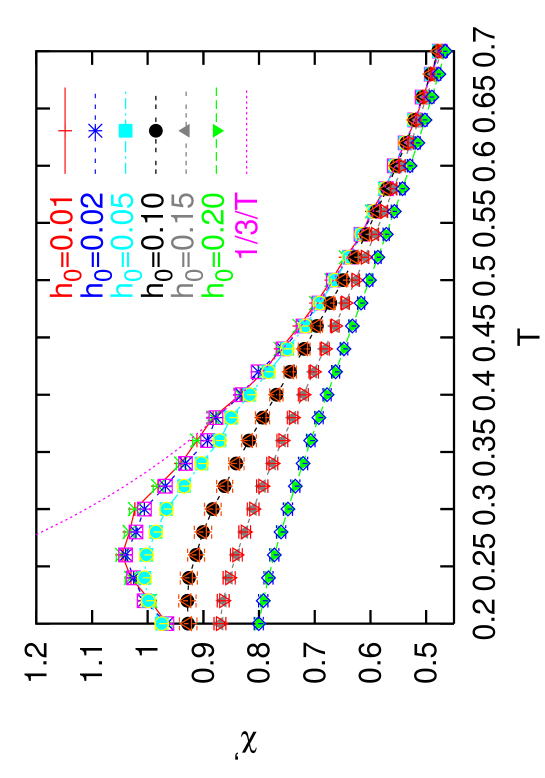
Figure 1: $\chi^{\prime}$ vs. $T$ for $L=10$, $P=50000$ and for varying value of the amplitude of magnetic field $h_{0}=0.02,0.05,0.10,0.15$ and $0.20$ (from bottom to top).

For each frequency $\omega$, we determine the temperature $T_{m}$ corresponding to the maximum of the in-phase susceptibility $\chi^{\prime}$ [15, 16]. This temperature determines the relaxation time $\tau(T_{m})=P$. Alternatively, one could also define $T_{m}$ as the value of the temperature at which an inflection point is observed in the out-of-phase susceptibility $\chi^{\prime\prime}$. Next, one can determine the static transition temperature as well as the critical exponent $z\nu$ using the scaling relation

$$\tau(T)\simeq c(T-T_{c})^{-z\nu}\;.$$ (7)

where $c$ is a constant. In a previous work [21], we had employed this method to study the Ising spin-glass model and the Heisenberg spin-glass model. Our findings, for the Ising case, was in very good agreement with a previous numerical study [16, 17] as well as with experimental results [18, 19, 15, 20]. For the Heisenberg case, our conclusion was that we had data compatible with a zero temperature divergence $\tau(T)\simeq T^{-z\nu}$ with a value of $z\nu\simeq 5.8$. In the present work, we reconsider more carefully the Heisenberg case. In AC susceptibility measurements there are two effects that must be carefully evaluated: finite-size effects and the amplitude of the AC field. Finite-size effects become particularly important as we move close to the critical temperature where the correlation length diverges. Since one has no direct access to the correlation length, one must be sure that the size considered is large enough. The amplitude of the magnetic field $h_{0}$ is also important as we want to keep our measurements in the linear response regime. Already for the Ising model [16], it was observed that a too large value of $h_{0}$ can affect the measurements. But in the case of the Ising spin-glass model, it is only for rather large values of the magnetic field $h_{0}$ that deviations were observed in simulations, typically for $h_{0}\simeq 0.4$. Here on the contrary, we will see that one needs to adjust the value of $h_{0}$ as a function of the frequency. The lower the frequency, then the lower the temperature that we want to probe, and the lowest the magnetic field must be. For the lowest frequency that we simulated, $\omega=1/150000$, we need to reduce the amplitude of the magnetic field to $h_{0}=0.01$. In Fig. 1 we show susceptibility values obtained for $L=10$ and $P=1/\omega=50000$, that is a rather small frequency. We can see how the position of the maximum is strongly affected by the value of $h_{0}$. It is only for values of $h_{0}\leq 0.02$ that the maximum converges to $T\simeq 0.26$. However the largest value of $h_{0}$ up to which we can locate the maximum of $\chi^{\prime}$ for a given $P$ does not seem to depend much on the size considered. Most of the simulation time has been spent at determining $h_{0}$ for each frequency. This was done by repeating, for each frequency, the measurements as shown in Fig.1 for decreasing values of $h_{0}$. The values of $h_{0}$ that we obtained are $0.05$ for $P\leq 5000$, $0.02$ for $P=15000,50000$ and $0.01$ for $P=150000$.

In practice, the fact that one needs to reduce the amplitude of the applied AC field has an important consequence. Indeed, fluctuations in the measured susceptibility increase very fast as we decrease $h_{0}$, as could be expected from (4,5). Thus, to reduce the errors on the value of $\chi^{\prime},\chi^{\prime\prime}$, one needs to increase the number of simulated samples. Consequently, since $h_{0}$ has to be reduced as one increases/decreases the value of the period/frequency, one must simulate a steadily larger number of samples as the size of the system increases.

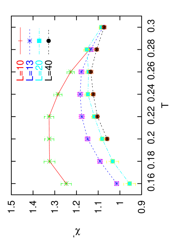
Figure 2: In-phase susceptibility as function of temperature, for $h=0.01$, $P=150000$ and for $L=10,13,20$ and $40$ (from top to bottom).

In Fig. 2 we show $\chi^{\prime}$ as a function of the temperature for $P=150000$, $h_{0}=0.01$ and for different sizes at the lowest frequency $\omega=1/P=1/150000$. It emerges from Fig. 2 that finite-size effects are very important and strongly influence the position of the maximum of the susceptibility. For $L=10$, the maximum is located at $\simeq 0.20$, while for $L=13$ it has moved to $\simeq 0.24$ and then it stabilizes close to $\simeq 0.26$ for $L=20$, apparently not changing anymore for larger sizes. Thus it seems that finite-size corrections can be very important, meaning that the correlation length must be rather large. Although the same type of behavior is also observed at other frequencies, it becomes more evident as we move to lower frequencies. This might have been expected, as the correlation length increases when the temperature decreases. In practice, for all the simulations that we have performed, we always got the same susceptibility for $L=20$ and $L=40$, thus we expect that our measurements for these sizes are free of finite-size effects.

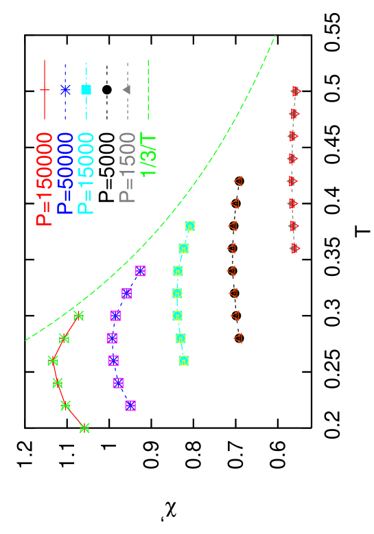
Figure 3: $\chi^{\prime}$ vs. $T$ for $P=1500,5000,15000,50000$ and $150000$ for $L=40$.

We will now present our main results for the critical behavior. We have computed the AC susceptibility for three sizes, $L=10,20,40$ and for $P=1500,5000,15000,50000$ and $150000$. For each of these sizes and periods, we have adjusted the value of the amplitude of the magnetic field $h_{0}$ in order to not see any shift of the maximum of $\chi^{\prime}$, as explained above. Also, we have checked that for each value of $P$, the susceptibility does not change between the sizes $L=20$ and $L=40$. The data that we obtained for $L=40$ is shown in Fig.3. We also see how the value of $T_{m}$ decreases as $\omega$ decreases. $T_{m}$ has been determined as the temperature for which there is a maximum in the susceptibility after fitting data to a parabolic form. In Fig.4, we show the temperature $T_{m}$ versus the period $P$. Data can be fitted to a power law (7) with $T_{c}=0.19\pm 0.04$ showing the existence of a finite-temperature transition in the zero-frequency limit. Since this value is very close to the one obtained for the chiral glass transition [8] and the spin-glass transition [13], we have repeated a fit but imposing the value for $T_{c}$ obtained in these works, i.e. $T_{c}=0.16$, in order to reduce the number of parameters of the fit. With this condition, we obtain a value of $z\nu=5\pm 0.5$ in good agreement with other estimates [8].

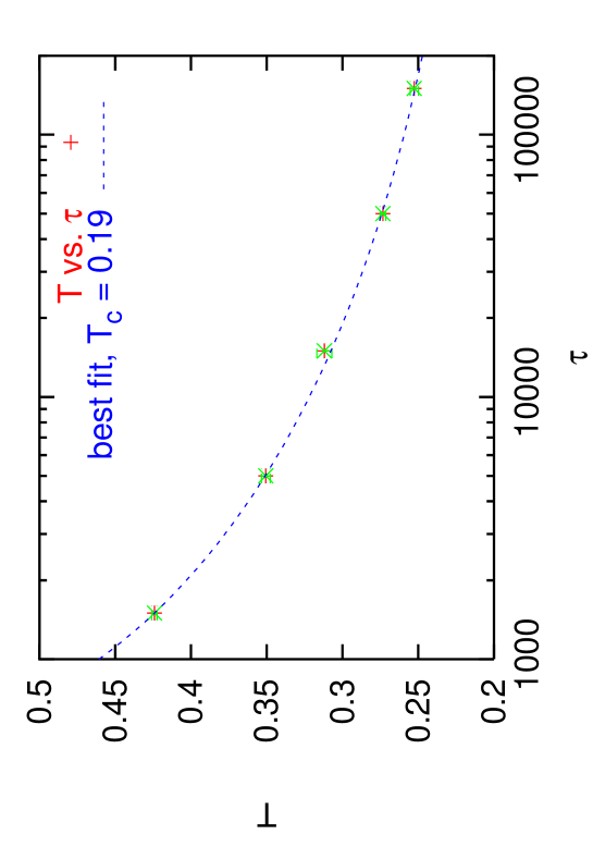
Figure 4: Temperature of the maximum of the in-phase susceptibility vs. the period $P$, for $L=40$. The discontinuous line is a best fit with (7).

In this paper we have performed AC susceptibility simulations for the Heisenberg spin-glass model. By carefully adjusting the value of the amplitude of the applied magnetic field $h_{0}$ as a function of the frequency considered, we have determined the relaxation time associated to each temperature. Extrapolating the relaxation time to the limit of zero frequency, we extract a value of critical temperature $T_{g}=0.19\pm 0.04$ compatible with either the values obtained for the chiral-glass transition [8] or the spin-glass transition [10, 11, 12, 13]. We also computed the exponent $z\nu=5.0\pm 0.5$ in good agreement with previous estimates [8] and experimental data for Heisenberg-like models [6, 15, 22]. Thus the simplest conclusion is that we are just observing a spin-glass transition at the same temperature as the chiral glass transition, in agreement with other recent studies [10, 11, 12, 13, 14]. But this is not the only possibility. Indeed, in the coupling/decoupling spin-chirality scenario of Kawamura [7], one expects that the chirality will couple at small distances with the spins. Thus, as far as one considers only small distances, one can observe physical phenomena expressed in term of spins while the transition is really on the chiral parameter. It is only for distances larger than some scale $L^{*}$ that spins and chirality decouple. This crossover length is related to the value of the period or frequency required to probe lengths of order $L^{*}$ in simulations. The value of $P$ is expected to be around $10^{5}-10^{6}$ [23] which is of the same order as the largest time that we probe in our simulation, $P=150000$. Thus we cannot, with the present simulations, exclude the possibility of a chiral-spin coupling scenario. Simulations for much lower frequencies are needed in order to probe this coupling/decoupling scenario and tell if indeed, the spin transition that we observe is due to the chiral glass transition or not.

Acknowledgements We want to thank F. Ricci-Tersenghi for discussions in the early stages of this work. One of the authors (MP) also wants to thank H. Kawamura for many helpful discussions and for the hospitality in Osaka University while part of this work was done. F. R has been supported by the Spanish grant BFM2001-3525, the STIPCO EEC network and the SPHINX program of the ESF.

References

- [1]
- [2] K. Binder and A. P. Young, Rev. Mod. Phys. 58, 801 (1986).
- [3] J. L. Tholence, Physica B 126, 157 (1984).
- [4] J. L. Tholence, Physica B 108, 1287 (1981).
- [5] K. Binder and A. P. Young, Phys. Rev. B 29, 2864 (1984).
- [6] J. Souletie and J. L. Tholence, Phys. Rev. B 32, 516 (1985).
- [7] H. Kawamura, Phys. Rev. Lett. 68, 3785 (1992); Phys. Rev. Lett. 80, 5421 (1998).
- [8] K. Hukushima and H. Kawamura, Phys. Rev. E 61, R1008 (2000).
- [9] J. A. Olive, A. P. Young and D. Sherrington, Phys. Rev. B 9, 6341 (1986).
- [10] F. Matsubara, T. Shirakura and S. Endoh, Phys. Rev. B 64, 092412 (2001).
- [11] T. Nakamura and S. Endoh, J. Phys. Soc. Jpn. 64, 2113 (2002).
- [12] F. Matsubara, T. Shirakura, S. Endoh and S. Takahashi, J. Phys, A 36, 10881 (2003).
- [13] L. W. Lee and A. P. Young, Phys. Rev. Lett. 90, 227203 (2003), Preprint cond-mat/0302371.
- [14] L. Berthier and A. P. Young, Preprint cond-mat/0312327.
- [15] E. Vincent, J. Hamman and M. Alba, Solid State Commun. 58, 57 (1986).
- [16] J.-O. Andersson, T. Jonsson and J. Mattson, Phys. Rev. B 54, 9912 (1996).
- [17] A. T. Ogielski, Phys. Rev. B 32, 7384 (1985).
- [18] N. Bontemps, J. Rajchenbach, R. V. Chamberlin and R. Orbach, Phys. Rev. B 30, 6514 (1984)
- [19] F. Matsukura, Y. Tazuke and T. Miyadai, J. Phys. Soc. Jpn. 58, 3355 (1989).
- [20] J. Mattsson, T. Jonsson, P. Nordblad, H. Aruga Katori and A. Ito, Phys. Rev. Lett. 74, 4305 (1995).
- [21] M. Picco, F. Ricci-Tersenghi and F. Ritort, Preprint cond-mat/0005541 v1, unpublished.
- [22] V. Dupuis, E. Vincent, J.-P. Bouchaud, J. Hammann, A. Ito and H. Aruga Katori, Phys. Rev. B 64, 174204 (2001), Preprint cond-mat/0104399.
- [23] K. Hukushima and H. Kawamura, to be published.