Perturbation Analysis of Superconductivity in the Trellis-Lattice Hubbard Model

Abstract

We investigate pairing symmetry and transition temperature in the trellis-lattice Hubbard model. We solve the Éliashberg equation using the third-order perturbation theory with respect to the on-site repulsion $U$. We find that a spin-singlet state is very stable in a wide range of parameters. On the other hand, when the electron number density is shifted from the half-filled state and the band gap between two bands is small, a spin-triplet superconductivity is expected. Finally, we discuss a possibility of unconventional superconductivity and pairing symmetry in Sr_14-xCa_xCu₂₄O₄₁.

1 Introduction

Quasi-one-dimensional superconductors have been studied and attracted our attention. Today, some quasi-one-dimensional superconductors, such as (TMTSF)₂X [1, 2] and $\beta$-Na_0.33V₂O₅ [3], were discovered, and their superconductivity has been investigated. In 1996, a superconducting transition in Sr_14-xCa_xCu₂₄O₄₁ was discovered at the transition temperature $T_{\mathrm{c}}\simeq 12\,$K under high pressure of approximately 3 GPa for $x=13.6$. [4] This material possesses a quasi-one-dimensional lattice structure called trellis lattice, which is Cu network connected by O orbitals similar to high-$T_{\mathrm{c}}$ superconductors as shown in Fig. 1(a). Actually, this material shows quasi-one-dimensional metallic behavior in an electric resistivity experiment.[5] The ratio of the resistivities $\rho_{a}/\rho_{c}$ is approximately 80 at ambient pressure, and is reduced approximately 30 under 3.5 GPa at $T\simeq 50$ K for $x=11.5$. Here, the Cu valence in this ladder can be changed from $+2.07$ ($x=0$) to $+2.24$ ($x=14$) by substituting Ca for Sr [6].

Recently, an NMR experiment has been performed in this material for $x=12$ by Fujiwara et al.  [7] From this experiment, an activated $T$ dependence of $1/T_{1}$ is observed at temperatures higher than $30\,$K, and it suggests that the spin gap is conformed. Below $30\,$K, $1/T_{1}T$ keeps constant and shows the Fermi liquid behavior. Moreover, $1/T_{1}$ has a small peak just below $T_{\mathrm{c}}$. It indicates that the superconducting gap structure is a fully gapped state in this material. On the other hand, the Knight shift does not change above and below $T_{\mathrm{c}}$. It suggests that a spin-triplet state is realized. But, since the paramagnetic contribution of Knight shift should be small owing to the effect of spin gap conformed at rather high temperatures, it might be difficult to detect the shift at $T_{\mathrm{c}}$ within the experimental accuracy.

The theoretical investigations for the possibility of unconventional superconductivity have been reported in the quasi-one-dimensional superconductors, such as (TMTSF)₂X, $\beta$-Na_0.33V₂O₅ and Sr_14-xCa_xCu₂₄O₄₁. The superconductivity in (TMTSF)₂X has been investigated within the fluctuation-exchange approximation (FLEX) [8] and the third-order perturbation theory (TOPT) [9]. The superconductivity in $\beta$-Na_0.33V₂O₅ has been investigated within TOPT. [10] Also, on the basis of the calculation within FLEX for the trellis-lattice Hubbard model, Kontani and Ueda indicated that a spin-singlet and fully gapped state is stable in Sr_14-xCa_xCu₂₄O₄₁. [11] In this paper, by using the third-order perturbation theory [12], we investigate in detail unconventional superconductivity in the trellis-lattice Hubbard model, keeping Sr_14-xCa_xCu₂₄O₄₁ in mind. In particular, we point out that the fully gapped state can be realized for unconventional superconductivity, and the spin-triplet state can be realized in a range of parameters.

2 Model

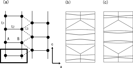
Figure 1: (a) Schematic figure of the lattice used in this calculation. $t_{i}(1\leq i\leq 3)$ is the hopping integral. The region enclosed by a rectangle is a primitive cell. The primitive cell topologycally composes a triangular lattice. (b) The Fermi surfaces for electron number density per ladder site $n=0.80$ and the hopping integrals $t_{2}=1.0$, $t_{3}=0.15$ are shown by the solid lines for $\varepsilon(k)+V(k)$ and by the dashed line for $\varepsilon(k)-V(k)$, respectively. Since the lattice is topologycally triangular lattice, the Brillouin zone is hexagonal. (c) The Fermi surface for $n=0.80$, $t_{1}=1.0$, $t_{2}=0.40$, $t_{3}=0.10$. In this case, the band gap is small.

Now, let us consider the lattice structure and the band structure in Sr_14-xCa_xCu₂₄O₄₁. We can consider the lattice structure with the Cu network called trellis lattice shown in Fig. 1(a). The unit cell is a thick-line rectangle, and contains two sites A and B. We use a simple tight-binding model. In this case, we consider three types of hopping integrals displayed in Fig. 1(a).

Here, we investigate in detail the nature of superconductivity in such a situation. We consider the quasi-one-dimensional two band repulsive Hubbard model.

$$\begin{split}H&=H_{0}+H_{\rm int},\end{split}$$ (1)

where

$$\begin{split}H_{0}&=\sum_{k,\sigma}\varepsilon(k)A^{\dagger}_{k\sigma}A_{k\sigma}+\sum_{k,\sigma}\varepsilon(k)B^{\dagger}_{k\sigma}B_{k\sigma}\\ &+\sum_{k,\sigma}V(k)A^{\dagger}_{k\sigma}B_{k\sigma}+\sum_{k,\sigma}V(k)B^{\dagger}_{k\sigma}A_{k\sigma},\end{split}$$ (2)

[14] and

$$\begin{split}H_{\rm int}&=\frac{U}{2N}\sum_{k_{i}}\sum_{\sigma\neq\sigma^{\prime}}A^{\dagger}_{k_{1}\sigma}A^{\dagger}_{k_{2}\sigma^{\prime}}A_{k_{3}\sigma^{\prime}}A_{k_{4}\sigma}\delta_{k_{1}+k_{2},k_{3}+k_{4}}\\ &+\frac{U}{2N}\sum_{k_{i}}\sum_{\sigma\neq\sigma^{\prime}}B^{\dagger}_{k_{1}\sigma}B^{\dagger}_{k_{2}\sigma^{\prime}}B_{k_{3}\sigma^{\prime}}B_{k_{4}\sigma}\delta_{k_{1}+k_{2},k_{3}+k_{4}}.\end{split}$$ (3)

From the tight binding approximation,

$$\begin{split}&\varepsilon(k)=-2t_{1}\cos(k_{c}),\\ &V(k)=|-t_{2}-2t_{3}\cos(k_{c}/2)e^{i\sqrt{3}k_{a}/2}|.\end{split}$$ (4)

Here, $A_{k,\sigma}$ and $B_{k,\sigma}$($A_{k,\sigma}^{\dagger}$ and $B_{k,\sigma}^{\dagger})$ are the annihilation (creation) operator for the electron at A and B site, respectively. To obtain two bands, we transform $A_{k,\sigma}^{({\dagger})}$, $B_{k,\sigma}^{({\dagger})}$ into $a_{k}^{({\dagger})},b_{k}^{({\dagger})}$ as

$$\begin{split}a_{k}^{({\dagger})}&=\frac{1}{\sqrt{2}}A_{k}^{({\dagger})}+\frac{1}{\sqrt{2}}B_{k}^{({\dagger})},\\ b_{k}^{({\dagger})}&=-\frac{1}{\sqrt{2}}A_{k}^{({\dagger})}+\frac{1}{\sqrt{2}}B_{k}^{({\dagger})}.\end{split}$$ (5)

With this transformation, $H_{0}$ is transformed into

$$\begin{split}H_{0}=\sum_{k,\sigma}(\varepsilon(k)+V(k))a^{\dagger}_{k\sigma}a_{k\sigma}+\sum_{k,\sigma}(\varepsilon(k)-V(k))b^{\dagger}_{k\sigma}b_{k\sigma}.\end{split}$$ (6)

Thus, we obtain two bands, $\varepsilon(k)+V(k)$ and $\varepsilon(k)-V(k)$. We use $t_{1}=1.0$ as an energy unit. In the previous calculation within FLEX [11], $t_{2}=1.0$ and $t_{3}=0.15$ are used to fit the band structure calculated within the local-density approximation [13]. In the calculation, the electron number density per ladder site $n=1.0$ is assumed. It means that the valence of Cu is $+2.0$. On the other hand, we use the hopping integrals $t_{2}$, $t_{3}$ and electron number density per ladder site $n$ as a parameter in this calculation. $t_{2}$ is a measure of the band gap between two bands, and $t_{3}$ is related to one-dimensionality. We show typical quasi-one-dimensional Fermi surfaces in Fig. 1(b) and (c). We show the Fermi surface for $t_{2}=1.0$, $t_{3}=0.15$, $n=0.80$ in Fig. 1(b), and for $t_{2}=0.40$, $t_{3}=0.10$, $n=0.80$ in Fig. 1(c), respectively. Actually, the band gap is small in Fig. 1(c).

3 Formulation

We apply the third-order perturbation theory with respect to $U$ to our model. The diagrams in the normal self-energy are shown in Fig. 2.

Figure 2: The diagrams in the normal self-energy. The solid and the broken lines represent $G^{(0)}_{\alpha\beta}(k)$ and $U$, respectively.

The normal self-energy is given by

$$\begin{split}&\Sigma^{\rm N}_{\alpha\beta}(k)=\frac{T}{N}\sum_{k^{\prime},\gamma}[\chi^{(0)}_{\alpha\beta}(k-k^{\prime})G^{(0)}_{\alpha\beta}(k^{\prime})U^{2}+\\ &(\chi^{(0)}_{\alpha\gamma}(k-k^{\prime})\chi^{(0)}_{\gamma\beta}(k-k^{\prime})+\phi^{(0)}_{\alpha\gamma}(k+k^{\prime})\phi^{(0)}_{\gamma\beta}(k+k^{\prime}))\\ &\times G^{(0)}_{\alpha\beta}(k^{\prime})U^{3}],\end{split}$$ (7)

where

$$\begin{split}&G^{(0)}_{\alpha\beta}(k)=\frac{1}{2}(G^{(0)}_{+}(k)+G^{(0)}_{-}(k))\quad(\alpha=\beta),\\ &G^{(0)}_{\alpha\beta}(k)=\frac{1}{2}(G^{(0)}_{+}(k)-G^{(0)}_{-}(k))\quad(\alpha\neq\beta),\\ &G^{(0)}_{\pm}(k)=\frac{1}{i\omega_{n}-(\varepsilon(\mbox{\boldmath$k$})\pm V(\mbox{\boldmath$k$}))+\mu},\\ &\chi^{(0)}_{\alpha\beta}(q)=-\frac{T}{N}\sum_{k}G^{(0)}_{\alpha\beta}(k)G^{(0)}_{\beta\alpha}(q+k),\\ &\phi^{(0)}_{\alpha\beta}(q)=-\frac{T}{N}\sum_{k}G^{(0)}_{\alpha\beta}(k)G^{(0)}_{\alpha\beta}(q-k).\end{split}$$ (8)

$G^{(0)}_{\alpha\beta}(k)$ with the short notation $k=(\mbox{\boldmath$k$},\omega_{n})$ represents the bare Green’s function. $\alpha$ and $\beta$ represent A or B. Here,

$$\begin{split}&\Sigma^{\rm N}_{\rm AA}(k)=\Sigma^{\rm N}_{\rm BB}(k),\\ &\Sigma^{\rm N}_{\rm AB}(k)=\Sigma^{\rm N}_{\rm BA}(k).\end{split}$$ (9)

Since the first-order normal self-energy is constant, it can be included by the chemical potential $\mu$. The dressed Green’s function $G_{\alpha\beta}(k)$ is given by

$$\begin{split}&G_{\alpha\beta}(k)=\frac{1}{2}(G_{+}(k)+G_{-}(k))\quad(\alpha=\beta),\\ &G_{\alpha\beta}(k)=\frac{1}{2}(G_{+}(k)-G_{-}(k))\quad(\alpha\neq\beta),\\ &G_{\pm}(k)=\frac{1}{(i\omega_{n}-(\varepsilon(\mbox{\boldmath$k$})\pm V(\mbox{\boldmath$k$}))-\Sigma^{\rm N}_{\pm}(k)+\mu+\delta\mu)},\\ &\Sigma^{\rm N}_{\pm}(k)=\Sigma^{\rm N}_{\rm AA}(k)\pm\Sigma^{\rm N}_{\rm AB}(k).\end{split}$$ (10)

Here, the chemical potential $\mu$ and the chemical potential shift $\delta\mu$ are determined so as to fix the electron number density per ladder site $n$,

$$\begin{split}n=\frac{T}{N}\sum_{k,\gamma}G^{(0)}_{\gamma\gamma}(k)=\frac{T}{N}\sum_{k,\gamma}G_{\gamma\gamma}(k).\end{split}$$ (11)

We also expand the effective pairing interaction up to the third order with respect to $U$. The diagrams of effective pairing interaction are shown in Fig. 3.

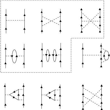
Figure 3: The diagrams of pairing interaction part. The diagrams enclosed by the dashed line are called the RPA-like terms. The other diagrams are the vertex corrections.

For the spin-singlet state, the effective pairing interaction is given by

$$\begin{split}&V^{\rm Singlet}_{\alpha\beta,\alpha^{\prime}\beta^{\prime}}(k;k^{\prime})\\ &=V^{\rm RPA\,Singlet}_{\alpha\beta,\alpha\beta}(k;k^{\prime})+V^{\rm Vertex\,Singlet}_{\alpha\beta,\alpha\gamma}(k;k^{\prime}),\end{split}$$ (12)

where

$$\begin{split}&V^{\rm RPA\,Singlet}_{\alpha\beta,\alpha\beta}(k;k^{\prime})=U\delta_{\alpha\beta}+U^{2}\chi^{(0)}_{\alpha\beta}(k-k^{\prime})\\ &+2U^{3}\chi^{(0)}_{\alpha\gamma}(k-k^{\prime})\chi^{(0)}_{\gamma\beta}(k-k^{\prime}),\end{split}$$ (13)

and

$$\begin{split}&V^{\rm Vertex\,Singlet}_{\alpha\beta,\alpha\gamma}(k;k^{\prime})=2(T/N)\mathrm{Re}\Big{[}\sum_{k_{1}}G^{(0)}_{\beta\alpha}(k_{1})\\ &\times(\chi^{(0)}_{\beta\gamma}(k+k_{1})-\phi^{(0)}_{\beta\gamma}(k+k_{1}))G^{(0)}_{\alpha\gamma}(k+k_{1}-k^{\prime})U^{3}\Big{]}.\end{split}$$ (14)

For the spin-triplet state,

$$\begin{split}&V^{\rm Triplet}_{\alpha\beta,\alpha^{\prime}\beta^{\prime}}(k;k^{\prime})\\ &=V^{\rm RPA\,Triplet}_{\alpha\beta,\alpha\beta}(k;k^{\prime})+V^{\rm Vertex\,Triplet}_{\alpha\beta,\alpha\gamma}(k;k^{\prime}),\end{split}$$ (15)

where

$$\begin{split}V^{\rm RPA\,Triplet}_{\alpha\beta,\alpha\beta}(k;k^{\prime})=-U^{2}\chi^{(0)}_{\alpha\beta}(k-k^{\prime}),\end{split}$$ (16)

and

$$\begin{split}&V^{\rm Vertex\,Triplet}_{\alpha\beta,\alpha\gamma}(k;k^{\prime})=2(T/N)\mathrm{Re}\Big{[}\sum_{k_{1}}G^{(0)}_{\beta\alpha}(k_{1})\\ &\times(\chi^{(0)}_{\beta\gamma}(k+k_{1})+\phi^{(0)}_{\beta\gamma}(k+k_{1}))G^{(0)}_{\alpha\gamma}(k+k_{1}-k^{\prime})U^{3}\Big{]}.\end{split}$$ (17)

Here, $V^{\rm RPA\,Singlet\,(Triplet)}_{\alpha\beta,\alpha\beta}(k,k^{\prime})$ is called the RPA-like terms and $V^{\rm Vertex\,Singlet\,(Triplet)}_{\alpha\beta,\alpha\gamma}(k,k^{\prime})$ is called the vertex corrections. Near the transition point, the anomalous self-energy $\Delta_{\alpha\beta}(k)$ satisfies the linearized Éliashberg equation,

$$\begin{split}&\lambda_{\rm max}\Delta_{\alpha\beta}(k)\\ &=-\frac{T}{N}\sum_{k^{\prime},\gamma}V_{\alpha\beta,\alpha^{\prime}\beta^{\prime}}(k;k^{\prime})F_{\alpha^{\prime}\beta^{\prime}}(k^{\prime}),\\ &=-\frac{T}{N}\sum_{k^{\prime},\gamma,\alpha^{\prime\prime},\beta^{\prime\prime}}V_{\alpha\beta,\alpha^{\prime}\beta^{\prime}}(k;k^{\prime})G_{\alpha^{\prime}\alpha^{\prime\prime}}(k^{\prime})G_{\beta^{\prime}\beta^{\prime\prime}}(-k^{\prime})\Delta_{\alpha^{\prime\prime}\beta^{\prime\prime}}(k^{\prime})\end{split}$$ (18)

[15] where, $V_{\alpha\beta,\alpha^{\prime}\beta^{\prime}}(k;k^{\prime})$ is $V^{\rm Singlet}_{\alpha\beta,\alpha^{\prime}\beta^{\prime}}(k;k^{\prime})$ or $V^{\rm Triplet}_{\alpha\beta,\alpha^{\prime}\beta^{\prime}}(k;k^{\prime})$. Here, $F_{\alpha^{\prime}\beta^{\prime}}(k^{\prime})$ is anomalous Green’s function, and $\lambda_{\rm max}$ is the largest positive eigenvalue. Then, the temperature at $\lambda_{\rm max}=1$ corresponds to $T_{\rm c}$. By estimating $\lambda_{\rm max}$, we can determine which type of pairing symmetry is stable. For numerical calculations, we take 128 $\times$ 128 $k$-meshes for twice space of the first Brillouin zone and 2048 Matsubara frequencies.

4 Numerical results

4.1 Dependence of $\lambda_{\rm max}$ on the parameters $t_{2}$ and $t_{3}$

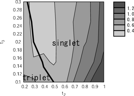
Figure 4: A contour plot of $\lambda_{\rm max}$ as a function of $t_{2}$ and $t_{3}$ in the case of $T=0.01$, $n=0.80$ and $U=4.0$. In the right hand side region of the thick line, a spin-singlet state is stable, and in the left hand side region of the thick line, a spin-triplet state is stable.

Fig. 4 is a contour plot of $\lambda_{\rm max}$ as a function of $t_{2}$ and $t_{3}$ in the case of $T=0.01$, $n=0.80$ and $U=4.0$. In the dark region, the state is stable. In the right hand side region of the thick line, a spin-singlet state is stable, and in the left hand side region of the thick line, a spin-triplet state is stable. When $t_{2}$ is large, a spin-singlet state is very stable. On the other hand, when $t_{2}$ is small, a spin-triplet state is stable. Therefore, a spin-triplet state is stable when the band gap between two band is small. We discuss this result later in Sec. 5. For $t_{3}<0.1$, the mass enhancement factor is much smaller than unity. Therefore, reliable numerical calculations in this framework can not be obtained in the range of $t_{3}<0.1$.

4.2 Temperature dependence

Figure 5: Temperature dependence of $\lambda_{\rm max}$ for a spin-singlet (or spin-triplet) state in the case of $t_{2}=1.0$, $t_{3}=0.15$, $n=0.80$ and $U=3.2$. The line with black circles (squares) is the temperature dependence for the spin-singlet (spin-triplet) state obtained using the third-order perturbation theory. The spin-singlet state is more stable than the spin-triplet state in this case.

Figure 6: Temperature dependence of $\lambda_{\rm max}$ for spin-singlet (or spin-triplet) state in the case of $t_{2}=0.40$, $t_{3}=0.10$, $n=0.80$ and $U=4.1$. The line with black circles (square) is the result for the spin-singlet (spin-triplet) state obtained using the third-order perturbation theory. The spin-triplet state is more stable than the spin-singlet state in this case. The line with the white circles (square) is the result for spin-singlet (spin-triplet) state without the third-order terms of the pairing interaction.

In Fig. 5, we show temperature dependences of $\lambda_{\rm max}$ in the case with $t_{2}=1.0$, $t_{3}=0.15$ $n=0.80$ and $U=3.2$. Also, in Fig. 6, we show temperature dependences for $\lambda_{\rm max}$ in the case with $t_{2}=0.40$, $t_{3}=0.10$, $n=0.80$ and $U=4.1$. With decreasing temperature, $\lambda_{\rm max}$ increases. In Fig. 5, the spin-singlet state is stable. On the other hand, in Fig. 6, the spin-triplet state is stable. These states possess almost the same transition temperature, $T_{\mathrm{c}}\simeq 0.003$, respectively. If we assume that the bandwidth $W\sim 6$ corresponds to $2\,{\rm eV}$, then $T_{\mathrm{c}}\sim 10\,{\rm K}$ is obtained in almost accordance with the experimental value for Sr_14-xCa_xCu₂₄O₄₁. In Fig. 6, we also show the results for $\lambda_{\rm max}$ obtained without the pairing interaction due to the third-order terms. We can see that the vertex corrections are important for stabilizing the spin-triplet state from the comparison.

4.3 Dependence of $\lambda_{\rm max}$ on the parameters $t_{2}$ and $n$

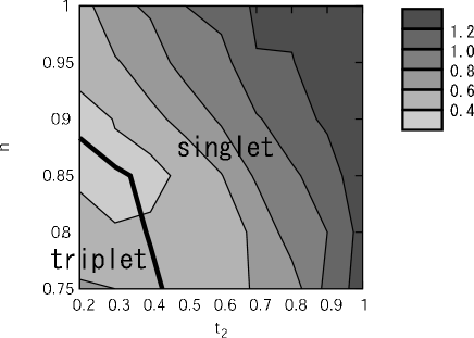
Figure 7: A contour plot of $\lambda_{\rm max}$ as a function of $t_{2}$ and $n$ in the case of $t_{3}=0.15$, $T=0.01$ and $U=4.0$. In the right hand side region of the thick line, a spin-singlet state is stable, and in the left hand side region of the thick line, a spin-triplet state is stable.

Fig. 7 is a contour plot of $\lambda_{\rm max}$ as a function of $t_{2}$ and $n$ in the case of $t_{3}=0.15$, $T=0.01$ and $U=4.0$. When $t_{2}$ is large, a spin-singlet state is very stable like the above case in Sec. 4.1. On the other hand, if $t_{2}$ is small and $n$ is shifted from the half-filled state, a spin-triplet state is stable. Thus, the spin-triplet state is suppressed in the vicinity of the half-filled state, and it is stable rather far from the half-filled state. This tendency is a general property. The pairing interaction important for the spin-triplet state originates from the third-order terms which vanishes in the case with the particle-hole symmetry. Therefore, $\lambda_{\rm max}$ is reduced due to approximate particle-hole symmetry near the half-filled state.

4.4 Dependence of $\lambda_{\rm max}$ on the parameters $t_{2}$ and $U$

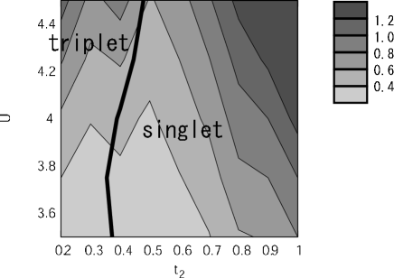
Figure 8: A contour plot of $\lambda_{\rm max}$ as a function of $t_{2}$ and $n$ in the case of $t_{3}=0.15$, $T=0.01$, and $U=4.0$. In the right hand side region of the thick line, a spin-singlet state is stable, and in the left hand side region of the thick line, a spin-triplet state is stable.

Fig. 8, is a contour plot of $\lambda_{\rm max}$ as a function of $t_{2}$ and $U$ in the case of $t_{3}=0.15$, $T=0.01$ and $n=0.80$. When $t_{2}$ is large, a spin-singlet state is very stable like the above case in Sec. 4.1. On the other hand, when $U$ becomes large, $\lambda_{\rm max}$ becomes large. But the stable symmetry does not depend on the magnitude of $U$ so much in this strongly correlated region. On the other hand, from the result of renormalization group approach [16] for $t_{3}=0$ and $U\rightarrow 0^{+}$, the spin-singlet state is stable for any values of $t_{2}$ and $n$. It does not contradict this result within the perturbation theory. When $U$ is very small, the vertex corrections are negligible which is important for the stabilization of the spin-triplet state. Therefore, when $U$ is very small, the spin-singlet state seems to be dominant from the results without the third-order terms of the pairing interaction. However, numerical calculation is difficult since the eigenvalue is very small in this case.

4.5 Momentum dependence of the anomalous self-energy

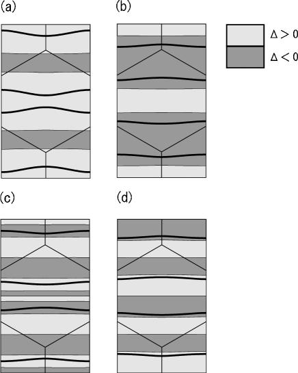
Figure 9: (a),(b) Contour plots of the anomalous self-energy $\Delta(k)=0$ for the spin-singlet state in the case of $t_{2}=1.0$, $t_{3}=0.15$, $T=0.01$, $n=0.80$ and $U=4.0$. The thick lines represent the Fermi surfaces. The spin-singlet state is a fully gapped state. (c),(d) Contour plots of the anomalous self-energy $\Delta(k)=0$ for the spin-triplet state in the case of $t_{2}=0.4$, $t_{3}=0.10$, $T=0.01$, $n=0.80$ and $U=4.0$. The thick lines represent the Fermi surfaces. The spin-triplet state is a fully gapped state.

From eq. (5), anomalous Green’s functions on the two bands are given by

$$\begin{split}&F_{+}(k)=|G_{+}(k)|^{2}\Delta_{+}(k)=F_{\rm AA}(k)+F_{\rm AB}(k),\\ &F_{-}(k)=|G_{-}(k)|^{2}\Delta_{-}(k)=F_{\rm AA}(k)-F_{\rm AB}(k).\end{split}$$ (19)

Therefore, anomalous self-energies on the two bands are given by

$$\begin{split}&\Delta_{+}(k)=\Delta_{\rm AA}(k)+\Delta_{\rm AB}(k),\\ &\Delta_{-}(k)=\Delta_{\rm AA}(k)-\Delta_{\rm AB}(k).\end{split}$$ (20)

In Fig. 9, we show contour plots of the anomalous self-energy in the case of $T=0.01$, $n=0.80$ and $U=4.0$. In Fig. 9 (a) and (b), a spin-singlet case for $t_{2}=1.0$, $t_{3}=0.15$, and in Fig. 9 (c) and (d), a spin-triplet case for $t_{2}=0.40$, $t_{3}=0.10$ are shown. The thick lines represent the Fermi surfaces. For the spin-singlet state, the momentum dependence of the anomalous self-energy on the Fermi surface is a fully gapped state, and the signs of the anomalous self-energy on the Fermi surface for the two band are different. We discuss this result later in Sec. 5. For the spin-triplet state, the momentum dependence of the anomalous self-energy is also a fully gapped state.

5 Discussions

In this section we consider the physical origin of the results in Sec. 4. Hereafter, we only consider the RPA-like terms to understand the mechanism of stabilization for the spin-singlet state. Éliashberg equation is written by

$$\begin{split}\Delta_{\rm AA}(k)=-\frac{T}{N}\sum_{k^{\prime}}V_{\rm AA}(k,k^{\prime})F_{\rm AA}(k^{\prime}),\\ \Delta_{\rm AB}(k)=-\frac{T}{N}\sum_{k^{\prime}}V_{\rm AB}(k,k^{\prime})F_{\rm AB}(k^{\prime}).\end{split}$$ (21)

Here, we write $V^{\rm RPA\,Singlet}_{\rm AA,AA}(k,k^{\prime})$ and $V^{\rm RPA\,Singlet}_{\rm AB,AB}$ as $V_{\rm AA}(k,k^{\prime})$ and $V_{\rm AB}(k,k^{\prime})$, respectively. The Éliashberg equation for $\Delta_{+}(k)$ and $\Delta_{-}(k)$ are given by

$$\begin{split}&\Delta_{+}(k)=\Delta_{\rm AA}(k)+\Delta_{\rm AB}(k)\\ &=-\frac{T}{N}\sum_{k^{\prime}}\frac{1}{2}(V_{\rm AA}(k,k^{\prime})+V_{\rm AB}(k,k^{\prime}))F_{+}(k^{\prime})\\ &-\frac{T}{N}\sum_{k^{\prime}}\frac{1}{2}(V_{\rm AA}(k,k^{\prime})-V_{\rm AB}(k,k^{\prime}))F_{-}(k^{\prime})\\ &=-\frac{T}{N}\sum_{k^{\prime}}\frac{1}{2}(V_{\rm AA}(k,k^{\prime})+V_{\rm AB}(k,k^{\prime}))|G_{+}(k^{\prime})|^{2}\Delta_{+}(k^{\prime})\\ &-\frac{T}{N}\sum_{k^{\prime}}\frac{1}{2}(V_{\rm AA}(k,k^{\prime})-V_{\rm AB}(k,k^{\prime}))|G_{-}(k^{\prime})|^{2}\Delta_{-}(k^{\prime})\\ &=-\frac{T}{N}\sum_{k^{\prime}}\frac{1}{2}V_{\rm intra}(k,k^{\prime})|G_{+}(k^{\prime})|^{2}\Delta_{+}(k^{\prime})\\ &-\frac{T}{N}\sum_{k^{\prime}}\frac{1}{2}V_{\rm inter}(k,k^{\prime})|G_{-}(k^{\prime})|^{2}\Delta_{-}(k^{\prime}),\end{split}$$ (22)

$$\begin{split}&\Delta_{-}(k)=\Delta_{\rm AA}(k)-\Delta_{\rm AB}(k)\\ &=-\frac{T}{N}\sum_{k^{\prime}}\frac{1}{2}(V_{\rm AA}(k,k^{\prime})-V_{\rm AB}(k,k^{\prime}))F_{+}(k^{\prime})\\ &-\frac{T}{N}\sum_{k^{\prime}}\frac{1}{2}(V_{\rm AA}(k,k^{\prime})+V_{\rm AB}(k,k^{\prime}))F_{-}(k^{\prime})\\ &=-\frac{T}{N}\sum_{k^{\prime}}\frac{1}{2}(V_{\rm AA}(k,k^{\prime})-V_{\rm AB}(k,k^{\prime}))|G_{+}(k^{\prime})|^{2}\Delta_{+}(k^{\prime})\\ &-\frac{T}{N}\sum_{k^{\prime}}\frac{1}{2}(V_{\rm AA}(k,k^{\prime})+V_{\rm AB}(k,k^{\prime}))|G_{-}(k^{\prime})|^{2}\Delta_{-}(k^{\prime})\\ &=-\frac{T}{N}\sum_{k^{\prime}}\frac{1}{2}V_{\rm inter}(k,k^{\prime})|G_{+}(k^{\prime})|^{2}\Delta_{+}(k^{\prime})\\ &-\frac{T}{N}\sum_{k^{\prime}}\frac{1}{2}V_{\rm intra}(k,k^{\prime})|G_{-}(k^{\prime})|^{2}\Delta_{-}(k^{\prime}),\end{split}$$ (23)

where,

$$\begin{split}&V_{\rm intra}(k,k^{\prime})\equiv V_{\rm AA}(k,k^{\prime})+V_{\rm AB}(k,k^{\prime})\\ &V_{\rm inter}(k,k^{\prime})\equiv V_{\rm AA}(k,k^{\prime})-V_{\rm AB}(k,k^{\prime}).\end{split}$$ (24)

The pairing interaction which connects the anomalous self-energies on the intra band is $V_{\rm intra}(k,k^{\prime})\equiv V_{\rm AA}(k,k^{\prime})+V_{\rm AB}(k,k^{\prime})$ and that on the inter band is $V_{\rm inter}(k,k^{\prime})\equiv V_{\rm AA}(k,k^{\prime})-V_{\rm AB}(k,k^{\prime})$. Here,

$$\begin{split}&V_{\rm intra}(k,k^{\prime})=V_{\rm AA}(k;k^{\prime})+V_{\rm AB}(k;k^{\prime})\\ &=U+U^{2}(\chi^{(0)}_{\rm AA}(k-k^{\prime})+\chi^{(0)}_{\rm AB}(k-k^{\prime}))\\ &+2U^{3}(\chi^{(0)}_{\rm AA}(k-k^{\prime})+\chi^{(0)}_{\rm AB}(k-k^{\prime}))^{2}\\ &=U+U^{2}\chi^{(0)}_{\rm intra}(k-k^{\prime})+2U^{3}\chi^{(0)}_{\rm intra}(k-k^{\prime})^{2},\\ &V_{\rm inter}(k,k^{\prime})=V_{\rm AA}(k,k^{\prime})-V_{\rm AB}(k;k^{\prime})\\ &=U+U^{2}(\chi^{(0)}_{\rm AA}(k-k^{\prime})-\chi^{(0)}_{\rm AB}(k-k^{\prime}))\\ &+2U^{3}(\chi^{(0)}_{\rm AA}(k-k^{\prime})-\chi^{(0)}_{\rm AB}(k-k^{\prime}))^{2}\\ &=U+U^{2}\chi^{(0)}_{\rm inter}(k-k^{\prime})+2U^{3}\chi^{(0)}_{\rm inter}(k-k^{\prime})^{2},\end{split}$$ (25)

where,

$$\begin{split}&\chi_{\rm intra}^{(0)}(q)\equiv\chi^{(0)}_{\rm AA}(q)+\chi^{(0)}_{\rm AB}(q),\\ &\chi_{\rm inter}^{(0)}(q)\equiv\chi^{(0)}_{\rm AA}(q)-\chi^{(0)}_{\rm AB}(q).\end{split}$$ (26)

Therefore, $V_{\rm intra}(k,k^{\prime})$ and $V_{\rm inter}(k,k^{\prime})$ are composed of $\chi_{\rm intra}^{(0)}(k-k^{\prime})\equiv\chi^{(0)}_{\rm AA}(k-k^{\prime})+\chi^{(0)}_{\rm AB}(k-k^{\prime})$ and $\chi_{\rm inter}^{(0)}(k-k^{\prime})\equiv\chi^{(0)}_{\rm AA}(k-k^{\prime})-\chi^{(0)}_{\rm AB}(k-k^{\prime})$, respectively. Here,

$$\begin{split}&\chi_{\rm intra}^{(0)}(q)=\chi_{\rm AA}^{(0)}(q)+\chi_{\rm AB}^{(0)}(q)\\ &=-\frac{T}{N}\sum_{k^{\prime}}\frac{1}{2}(G_{+}^{(0)}(k^{\prime})G_{+}^{(0)}(q+k^{\prime})+G_{-}^{(0)}(k^{\prime})G_{-}^{(0)}(q+k^{\prime})),\\ &\chi_{\rm inter}^{(0)}(q)=\chi_{\rm AA}^{(0)}(q)-\chi_{\rm AB}^{(0)}(q)\\ &=-\frac{T}{N}\sum_{k^{\prime}}(G_{+}^{(0)}(k^{\prime})G_{-}^{(0)}(q+k^{\prime})).\end{split}$$ (27)

Therefore, $\chi_{\rm intra}^{(0)}(q)$ is the average of the bare susceptibility of the intra bands and $\chi_{\rm inter}^{(0)}(q)$ is the bare susceptibility of the inter bands.

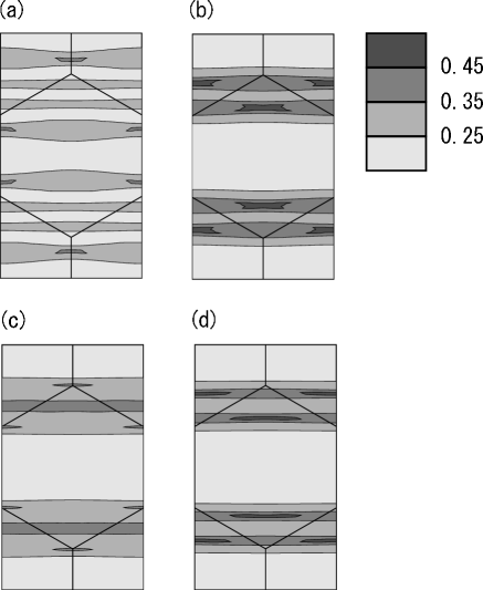
Figure 10: (a) A contour plot of $\chi_{\rm intra}^{(0)}(\mbox{\boldmath$q$},0)\equiv\chi_{\rm AA}^{(0)}(\mbox{\boldmath$q$},0)+\chi_{\rm AB}^{(0)}(\mbox{\boldmath$q$},0)$ in the case of $t_{2}=1.0$, $t_{3}=0.15$, $n=0.80$ and $T=0.01$. (b) A contour plot of $\chi_{\rm inter}^{(0)}(\mbox{\boldmath$q$},0)\equiv\chi_{\rm AA}^{(0)}(\mbox{\boldmath$q$},0)-\chi_{\rm AB}^{(0)}(\mbox{\boldmath$q$},0)$ in the case of $t_{2}=1.0$, $t_{3}=0.15$, $n=0.80$ and $T=0.01$. (c) A contour plot of $\chi_{\rm intra}^{(0)}(\mbox{\boldmath$q$},0)\equiv\chi_{\rm AA}^{(0)}(\mbox{\boldmath$q$},0)+\chi_{\rm AB}^{(0)}(\mbox{\boldmath$q$},0)$ in the case of $t_{2}=0.40$, $t_{3}=0.10$, $n=0.80$ and $T=0.01$. (d) A contour plot of $\chi_{\rm inter}^{(0)}(\mbox{\boldmath$q$},0)\equiv\chi_{\rm AA}^{(0)}(\mbox{\boldmath$q$},0)-\chi_{\rm AB}^{(0)}(\mbox{\boldmath$q$},0)$ in the case of $t_{2}=0.40$, $t_{3}=0.10$, $n=0.80$ and $T=0.01$. When the band gap between two band is large, $\chi_{\rm intra}^{(0)}(\mbox{\boldmath$q$},0)$ is small like the case (a). On the other hand, when the band gap between two band is small, $\chi_{\rm intra}^{(0)}(\mbox{\boldmath$q$},0)$ is large like the case (c). The spin-singlet state is stable in the case (a), and the spin-singlet state is unstable in the case (c).

Fig. 10 is contour plots of $\chi_{\rm intra}^{(0)}(\mbox{\boldmath$q$},0)$ and $\chi_{\rm inter}^{(0)}(\mbox{\boldmath$q$},0)$ in the cases of $t_{2}=1.0$, $t_{3}=0.15$, $n=0.80$, $T=0.01$ and for $t_{2}=0.40$, $t_{3}=0.10$, $n=0.80$, $T=0.01$, respectively. Since the Fermi surfaces have nesting property, they have quasi-one dimensional peaks. Since $\chi_{\rm intra}^{(0)}(\mbox{\boldmath$q$},0)$ is the average of the bare susceptibility of the intra bands, it is usually smaller than $\chi_{\rm inter}^{(0)}(\mbox{\boldmath$q$},0)$. But when the band gap between two bands is small, two nesting vectors of intra band become almost same. Therefore, $\chi_{\rm intra}^{(0)}(\mbox{\boldmath$q$},0)$ with small band gap is large compared with the case where the band gap between two bands is large. Actually, in Fig 10, when the band gap between two bands is large, $\chi_{\rm intra}^{(0)}(\mbox{\boldmath$q$},0)$ is small like the case (a). On the other hand, when the band gap between two bands is small, $\chi_{\rm intra}^{(0)}(\mbox{\boldmath$q$},0)$ is large like the case (c). By using the results in Fig. 10, we can understand the superconducting gap structure in Fig. 9 (a),(b) and the suppression of $\lambda_{\rm max}$ in the case where the band gap between two bands is small, as we explain in the following. From the structure in the Éliashberg equation, when $\chi_{\rm intra}^{(0)}(\mbox{\boldmath$q$},0)$ is much smaller than $\chi_{\rm inter}^{(0)}(\mbox{\boldmath$q$},0)$, in order to obtain a positive value of $\lambda_{\rm max}$, it is favorable that signs of $\Delta(k)$ on one band are different from its sign on another band. The structure of $\Delta(k)$ in Fig. 9 (a),(b) just becomes so. But, when the band gap between two bands is small, two nesting vectors of intra bands are almost same. Therefore, $\chi^{(0)}_{\rm intra}(\mbox{\boldmath$q$},0)$ becomes large and the spin-singlet state is suppressed by the conflict of the peaks of $\chi_{\rm intra}^{(0)}(\mbox{\boldmath$q$},0)$ and $\chi_{\rm inter}^{(0)}(\mbox{\boldmath$q$},0)$. Actually, in Fig. 10, when the band gap between two bands is large, $\chi_{\rm intra}^{(0)}(\mbox{\boldmath$q$},0)$ is small and the spin-singlet state is very stable like the case (a). On the other hand, when the band gap between two bands is small, $\chi_{\rm intra}^{(0)}(\mbox{\boldmath$q$},0)$ is large and the spin-singlet state is unstable like the case (c).

Finally, we discuss the pairing symmetry in Sr_14-xCa_xCu₂₄O₄₁. From this calculation, we can see that the spin-singlet and fully gapped state is very stable and is consistent with the calculation within FLEX [11]. On the other hand, when the electron number density is shifted from the half-filled state and the band gap between two bands is small, the spin-triplet and fully gapped state is stable. We cannot unfortunately determine the electronic structure under the pressure at present. In both cases, the fully gapped state is not contradict to the experiment of $1/T_{1}$. On the other hand, the Knight shift does not change above and below $T_{\mathrm{c}}$. It suggests that a spin-triplet state is realized. But, since the paramagnetic contribution of Knight shift should be small owing to the effect of spin gap conformed at rather high temperatures, it might be difficult to detect the shift at $T_{\mathrm{c}}$ within the experimental accuracy. Here, we discuss the ratio of hopping integrals. The ratio $t_{1}/t_{2}$ may be considered to be unity from almost equivalent spacings of the leg and the rung in this ladder. Experimentally, however, the ratio of the spin exchange coupling constant $J_{\rm leg}/J_{\rm rung}$ is about twice for related compounds. [17, 18] Here, $J_{\rm leg}$ and $J_{\rm rung}$ are related to $t_{1}$ and $t_{2}$, respectively. Moreover, the pressure might change the ratio $t_{1}/t_{2}$. Therefore, we can expect a flexible value for the ratio $t_{1}/t_{2}$.

6 Conclusion

In conclusion, we have investigated the pairing symmetry and the transition temperature on the basis of the trellis-lattice Hubbard model. We have solved the Éliashberg equation using the third-order perturbation theory with respect to the on-site repulsion $U$. We find that the spin-singlet state is strongly stable in a wide range of parameters. On the other hand, when the electron number density is shifted from the half-filled state and the band gap between two bands is small, the spin-triplet state is expected. Thus, we suggest the possibility of unconventional superconductivity in Sr_14-xCa_xCu₂₄O₄₁.

7 Acknowledgments

Numerical calculation in this work was carried out at the Yukawa Institute Computer Facility.

References

[1] For review, T. Ishiguro, K. Yamaji and G. Saito:
Organic Superconductors (Springer-Verlag, Heiderberg, 1998)
[2] D. Jérome and H. J. Schulz:
Adv. Phys. 31 (1982) 299.
[3] T. Yamauchi, Y. Ueda and N. Môri:
Phys. Rev. Lett. 89 (2002) 057002.
[4] M. Uehara, T. Nagata, J. Akimitsu, H. Takahashi, N. Môri and K. Kinoshita:
J. Phys. Soc. Jpn. 65 (1996) 2764
[5] T. Nagata, M. Uehara, J. Goto, J. Akimitsu, N. Motoyama, H. Eisaki, S. Uchida, H. Takahashi, T. Nakanishi, and N. Môri:
Phys. Rev. Lett. 81 (1998) 1090
[6] T. Osafune, N. Motoyama, H. Eisaki, and S. Uchida:
Phys. Rev. Lett. 78 (1997) 1980.
[7] N. Fujiwara, N. Môri, Y. Uwatoko, T. Matsumoto, N. Motoyama and S. Uchida:
Phys. Rev. Lett. 90 (2003) 137001.
[8] H. Kino and H. Kontani:
J. Phys. Soc. Jpn. 68 (1999) 1481.
[9] T. Nomura and K. Yamada:
J. Phys. Soc. Jpn. 70 (2001) 2694.
[10] S. Sasaki, H. Ikeda and K. Yamada:
J. Phys. Soc. Jpn. 73 (2004) 815.
[11] H. Kontani and K. Ueda:
Phys. Rev. Lett. 80 (1998) 5619.
[12] Y. Yanase, T. Jujo, T. Nomura, H. Ikeda, T. Hotta,
K. Yamada:
Phys. Rep. 387 (2003) 1.
[13] M. Arai, H. Tsunetsugu:
Phys. Rev. B 56 (1997) 4305
[14]
From the tight-binding model, is complex number, but phase factor can be included into the and
[15]
We assume and .
[16] L. Balents and M. P. A. Fisher:
Phys. Rev. B 53 (1996) 12133.
[17] D. C. Johnston:
Phys. Rev. B 54 (1996) 13009.
[18] T. Imai, K. R. Thurber, K. M. Shen, A. W. Hunt and
F. C. Chou:
Phys. Rev. Lett. 81 (1998) 220.