Reconstructing the Density of States by History-Dependent Metadynamics

Abstract

We present a novel method for the calculation of the energy density of states $D(E)$ for systems described by classical statistical mechanics. The method builds on an extension of a recently proposed strategy that allows the free energy profile of a canonical system to be recovered within a pre-assigned accuracy,[A. Laio and M. Parrinello, PNAS 2002]. The method allows a good control over the error on the recovered system entropy. This fact is exploited to obtain $D(E)$ more efficiently by combining measurements at different temperatures. The accuracy and efficiency of the method are tested for the two-dimensional Ising model (up to size 50x50) by comparison with both exact results and previous studies. This method is a general one and should be applicable to more realistic model systems.

It has long been recognized that all energy-related thermodynamic properties of a classical canonical system can be calculated once the energy density of states $D(E)$ is known. In fact, starting from the partition function $Z=\int dE\,D(E)e^{-\beta E}$, quantities like free energies, specific heats and phase transition temperatures can be computed in a straightforward manner. In principle, all canonical averages can be calculated through a multidimensional density of states. Due to this central role in equilibrium thermodynamics a variety of theoretical and computations studies have addressed the problem of how to obtain $D(E)$ (or, equivalently, the entropy profile $S(E)=\ln(D(E)$) in a reliable and efficient way.

In principle, $D(E)$ could be calculated from the histogram of the energies visited during a single “very long” constant-temperature simulationbennett . In practice, for any finite simulation only a limited energy windows is sampled so that the recovery of the system thermodynamics over a wide temperature range is unfeasible.

Several alternative strategies have been developed to remedy this shortcoming. For example the multiple histogram reweighting technique relies on performing several simulations at different temperatures, so as to explore different (overlapping) energy intervals multihisto . The various histograms are then optimally combined to obtain $D(E)$ over the union of the energy intervals. Another successful family of techniques aims at obtaining $D(E)$ by changing iteratively the probability with which the various energy levels are visited in stochastic dynamics until the recorded energy histogram is “flat”. Such methods include entropic sampling Lee , multicanonical and broad-histogram techniques techniques muca ; bhm and also the recent method of Wang and Landau wl01 .

These and similar techniques have proved to be very valuable in a variety of contexts hansmann ; hesse ; TROW , but there is still ample scope for alternative approaches that could provide improved efficiency and better error control. Here we propose to modify and extend the metadynamics method recently introduced by two of us hills for evaluating $D(E)$. The algorithm we introduce allows a good error control on the explored energy range. Moreover, although within our approach $D(E)$ could be reconstructed performing simulations at virtually any temperature, it is still possible to exploit the Boltzmann bias to focalize the computational effort for exploring the region of phase space of relevance for a temperature of interest (e.g. of a phase transition). In the following we will first describe this general strategy followed by its application to the typical reference case constituted by the two-dimensional Ising model.

The essence of the metadynamics approach is first to identify those relevant collective variables (CVs) that are difficult to sample. In other applicationshills a similar metodology was applied in order to observe a specific transition (e.g. a chemical reaction) in systems described by a complex atomistic Hamiltonian. At this scope CVs explicitly depending on the microscopic configuration of the system have been employed, like, e.g., coordination numbers or distances between specific atoms of the system. Here, we aim at reconstructing the canonical free-energy profile, $F(E)=E-T\,S(E)$ and the relevant variable is $E$ (which is also an explicit function of the microscopic configuration of the system). At each metadynamics step the system evolution is guided by the generalised force which combines the action of the thermodynamic force (which would trap the system in free-energy minima) $dF(E)/dE$ and a history-dependent one which disfavours system configurations already visited. The history-dependent potential, $F_{G}$, is constructed as a sum of Gaussians of width $\Delta E$ and height $w$ centred around each value of $E$ already explored during the dynamics. As shown in ref hills , $F_{G}$ fills in time the minima in the free energy surface and, in the limit of a long metadynamics $F(E)+F_{G}(E)$ tends to become flat as a function of $E$ and hence $-F_{G}(E)$ becomes an approximant of $F(E)$.

Clearly, the exact form of the metadynamics equations and the choice of the parameters $w$ and $\Delta E$ may affect significantly the accuracy of this estimate. Furthermore careful control of the error is essential for reconstructing a reliable density of states. This requires that the algorithm in ref. hills be substantially improved. The modified metadynamics equations are:

$$E_{G}^{t+1}=E^{t}+\Delta E\frac{f\left(E^{t}\right)}{\left|f\left(E^{t}\right)\right|}$$ (1)

$$E^{t+1}=E^{t}+\Delta E(1+\frac{\chi}{2})\frac{f\left(E^{t}\right)}{\left|f\left(E^{t}\right)\right|}$$ (2)

where $\chi$ is a random number between 0 and 1. The generalized force $f(E)$ is given by $f\left(E\right)=-{\partial\over\partial E}\left[F(E)+F_{G}^{t}(E)\right]$ with the history-dependent potential, $F^{t}_{G}$, defined as

$$F^{t}_{G}\left(E\right)=\sum_{u\leq t}w\,e^{-\frac{(E-E^{u}_{G})^{2}}{2\Delta E^{2}}}\ .$$ (3)

By displacing the center of the Gaussian $E_{G}^{t+1}$ with respect to the point of evaluation of the generalised force (equation 1), the added Gaussian maximally compensates $f(E^{t})$ and flattens $F+F_{G}$ around $E^{t}$. The energy step performed at every metadynamics iteration is chosen randomly in the interval between $\Delta E$ and $1.5\Delta E$ (equation 2) in order to reduce the correlation induced by the dynamics.

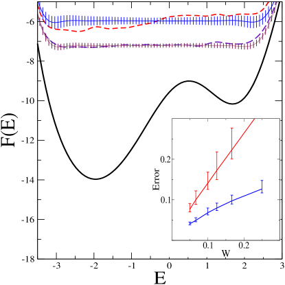
Figure 1: Example of reconstruction of a preassigned (analytic) free-energy profile (black curve), $F(E)$, by means of metadynamics runs consisting of 200 Gaussians of spread $\Delta E=0.4$ and height $w=0.16$. To mimic the uncertainty on the thermodynamic force encountered in stochastic simulations, a Gaussian noise of width 0.3 was added to $F^{\prime}(E)$. The broken red and indigo lines denote the filled profile, $\delta F(E)=F(E)-F_{R}(E)$, obtained respectively with an unsmoothed ($\tau_{c}=0$) and smoothed ($\tau_{c}=100$) metadynamics. Notice the shorter correlation lengths and smaller amplitudes of the fluctuations in the second case. The average and dispersion of $\delta F(E)$ were calculated (blue and brown lines wth error bars) for 1000 independent runs, revealing both the absence of biases in $F_{R}(E)$ and the constancy of the error except close to the boundaries. By changing $w$ and modifying the number of Gaussians so as to work at a constant filled free-energy volume, we calculated over the range $|E|<2.5$ the average, maximum and minimum values of $\delta F(E)$ measured over 1000 runs, see inset. The linear dependence of the error on $F_{R}$ is thus apparent both for the unsmoothed and smoothed metadynamics (red and blue respectively).

Finally, in order to further reduce the spatial correlations in $F_{G}$, we notice that when the metadynamics is terminated, say at position $E^{t}$, $F_{G}$ will present a bump in a region around $E^{t}$ whose spread depends on the correlation time of the metadynamics. This effect can be lessened if the contribution of the Gaussians placed at the end of the dynamics are weighted less. Therefore, after the metadynamics with constant $w$ is terminated we reconstruct the free energy from $F_{R}\left(E\right)=-\sum_{u\leq t}w\tanh\left(\frac{t-u}{\tau_{c}}\right)e^{-\frac{\left(E-E^{u}\right)^{2}}{2\Delta E^{2}}}$ where $\tau_{c}$ is taken to be larger than the typical time required to sweep the “filled” energy range. Other smoothing functions, such as $\min(1,\frac{t-u}{\tau_{c}})$ can, of course, also be chosen and have an analogous effect.

The modified metadynamics algorithm allows the efficient reconstruction of $F(E)$ in the explored energy range, within an error that is ultimately controlled only by the Gaussian’s height $w$. We demonstrate the quality of the algorithm by reconstructing an “ideal”, pre-assigned, $F\left(E\right)$ (see Fig. 1). If the method is void of systematic biases one would expect the quantity $\delta F\left(E\right)\equiv F_{R}\left(E\right)-F\left(E\right)$ to be, on average, constant throughout the filled energy range. Moreover, we would expect deviations from the constant average value to be of the order of $w$. These properties are confirmed by the results presented in the inset of Fig. 1, where the uniformity of the average value of $\delta F(E)$ is apparent, together with the constancy of its dispersion, $\sigma^{2}\left(E\right)=\langle\delta F\left(E\right)^{2}\rangle-\langle\delta F\left(E\right)\rangle^{2}$. The plots also illustrate the benefits of the “smoothing” procedure over the last part of the metadynamics trajectory, since this results in a decrease of the spread of $\delta F(E)$. As is visible in the inset of Fig. 1, the dispersion is further confirmed to be approximately proportional to $w$. An important fact is that near the boundaries of the explored energy interval $F_{R}(E)$ decays to zero and hence deviates from the true free energy. To identify the interval over which $F_{R}$ is reliable we need to ascertain if the number of Gaussians accumulated at a given energy $E$, $\approx|F_{R}(E)/w|$, is significantly larger than the minimal number of superposed Gaussians needed to produce the observed free energy derivative, $\approx F^{\prime}(E)/(w/\Delta E)$. In this work we have required that the ratio of the former to the latter be greater than 5.

We now use the algorithm described above to compute $D(E)$ for an $N$x$N$ two-dimensional Ising model with ferromagnetic nearest-neighbour interactions and periodic boundary conditions ising . In fact, exact expressions for S(E) are availablebeale and the error induced by the algorithm can be explicitly estimated and comparison with other approaches can be madewl01 .

Virtually the entire computational effort of the metadynamics is spent in estimating the thermodynamic forces $\partial F/\partial E$ at each energy value, $\bar{E}$, visited by the metadynamics. To respect the discrete nature of the system’s energy spectrum, the continuous value of $E^{t}$ produced by eq. (2) was discretized to the nearest energy level. Due to the discreteness of the energy spectrum, the thermodynamic force in $\bar{E}$ cannot be estimated by the Lagrange-multipliers technique described in Ref.hills , and is rather obtained using a centred difference approach. If $p_{1}$ and $p_{2}$ are the occupation probabilities of the two energy levels, $E_{1}$ and $E_{2}$ adjacent to $\bar{E}$ (we assume $|\bar{E}-E_{1}|=|\bar{E}-E_{2}|$), we have:

$${\partial F\over\partial E}|_{E=\bar{E}}={T\over(E_{2}-E_{1})}\,\ln{p_{1}\over p_{2}}\ .$$ (4)

$p_{1}$ and $p_{2}$ are evaluated with an umbrella-sampling strategy consisting of a Monte Carlo evolution of the system (Metropolis acceptance/rejection of single-spin flips) under the action of an effective Hamiltonian obtained by adding to the energy of a given spin configuration, $E$, the term $1/2\,K(E-\bar{E})^{2}$. A suitable choice of the parameter $K$ forces the system to explore the energy region around $\bar{E}$ thus populating appreciably both levels $E_{1}$ and $E_{2}$. The symmetry with respect to $\bar{E}$ of the added umbrella potential allows to calculate the thermodynamic force through the same eq. 4 with $p_{1}$ and $p_{2}$ being the fraction of times that the corresponding energy levels are encountered in $n$ statistically independent configurations picked with the modified canonical weight. For this purpose the Monte Carlo trajectory was sampled at intervals comparable to the autocorrelation time after having discarded a few tens of initial system sweeps. The MC sampling was stopped when the estimated uncertainty on the force note_binomial was equal to the maximum force introduced by a single Gaussian, $w\,\exp(-1/2)/\Delta E$. This choice ensures that, for large values of $t$, $f(\bar{E})$ is of the order of $w/\Delta E$. If the force is calculated with much greater accuracy the repeated superposition of the Gaussians would still lead to an uncertainty of order $w/\Delta E$ on $f(\bar{E})$.

By means of such a metadynamics it is therefore possible to reconstruct the free energy profile, $F_{R}(E,T)$. An estimator for the system entropy is given by $S_{R}(E)=[E-F_{R}(E,T)]/T$. The uncertainty over $F_{R}(E,T)$ is inherited by $S_{R}(E)$ whose a priori dispersion is thus of the order $w/T$. Thus, the expected error on the entropy profile is constant. This represents a major difference over standard reweighting techniques, where the accuracy on the calculated entropy usually deteriorates as one moves away from the free energy minima.

If the goal is to reconstruct $S(E)$ over a wide range of energy, it seems natural to combine the outcome of several meta-dynamics at various temperatures, in analogy with multiple-histogram techniquesmultihisto . In the following we shall indicate with $S_{R,i}$ the entropy reconstructed in the $i$th metadynamics carried out at temperature $T_{i}$ and with Gaussians of height $w_{i}$ and width $\delta_{i}$. Due to the temperature-dependence of the free energy, each run will typically explore a different energy range. The data obtained in the different metadynamics runs can be optimally combined to provide a single entropy estimate, $\tilde{S}$, over the union of the explored regionsmultihisto . To do so we recall that the entropy $S_{R,i}$ is known only up to an additive constant $c_{i}$ and that the uncertainty on $S_{R,i}$ is $\epsilon_{i}=w_{i}/T_{i}$ throughout the reliably-explored energy range.

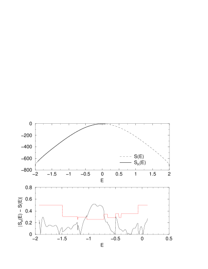
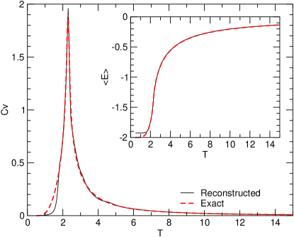
Figure 2: Results from the metadynamics runs carried out on the 32x32 Ising system. Top: the exact and reconstructed entropies. In both cases the entropy has been normalised so that $\sum_{E}\exp[S(E)]=1$. The abscissa indicates the energy per spin. Middle: Difference between the true and reconstructed entropy. The dispersion expected a priori on the reconstructed entropy is shown with a red line. Bottom: the exact and reconstructed specific heat and average energy (inset) as a function of temperature.

This leads us naturally to consider a maximum likelihood approach to obtain $\tilde{S}$ and the additive constants by minimizing the least-squares function,

$${\cal L}(\tilde{S},c_{1},...c_{n})=\sum_{i=1,n}\sum_{E}{|\tilde{S}(E)-S_{R,i}(E)-c_{i}|^{2}\over\epsilon_{i}^{2}}$$ (5)

where the first sum is carried over the various metadynamics runs and the second one runs over the system (discrete) energy levels with the proviso that $\epsilon_{i}$ is equal to infinity outside the reliable energy range. The determination of $\tilde{S}(E)$ through the minimization of ${\cal L}$ relies on the statistical independence of each term in the sum of equation (5). This is realized only approximately due to the existence of an intrinsic scale of autocorrelation for the reconstructed free-energy/entropy dictated by the correlation lenght of the metadynamics. Therefore, the minimization of (5) is meaningful provided that each energy value is covered by several metadynamics runs, each exploring an interval substantially larger than the Gaussian widths.

The requirement of stationarity for ${\cal L}$ leads to self-consistent equations which can be solved iteratively in terms of the $c_{i}$’s and $\tilde{S}(E)$. Despite the presence of the additive terms, $c_{i}$’s, which distinguish the present juxtaposition scheme from others already available, the self-consistent equations are simple both in their formulation and numerical implementation. Convergence to the solutions is typically reached in a few tens of iterations. The least-squares approach also allows the expected standard deviation of $\tilde{S}(E)$ to be calculated:

$$\sigma(\tilde{S}(E))^{-1/2}=\sum_{i=1..n}\epsilon_{i}(E)^{-2}\ .$$ (6)

The use of the reconstruction strategy is first illustrated for the 32x32 Ising model, see Fig. 2. The curve for the entropy, Fig. 2, results from the combination of runs at six temperatures, $T=$ 2, 2.6, 3.0, 3.4, 6.0 and 12.0. At each temperature 1000 Gaussians where used with $w/T\approx 0.5$, $\Delta E\approx 0.04$, $K\approx 0.4$ and $\tau_{c}=300$. The total computational effort required $7.5\,10^{5}$ MC sweeps. The comparison with the true system entropy reveals that $S(E)$ was correctly reconstructed throughout the explored energy range [-1.93; 1.93] (exploiting the ferro/antiferro symmetry) with an uncertainty that is approximately constant (its average being 0.17) and in agreement with the one expected a priori from eq. 6. The corresponding average relative error on $S(E)$ was 0.05%, similar to that obtained with a comparable number of sweeps in the recent and powerful approaches described in refs. muca ; wl01 .

Analogous runs were repeated for the 50x50 system using three temperatures, $T=2.6,4$ and $12$ and the same parameters as before. By using 2.2 $10^{6}$ Monte Carlo sweeps $S(E)$ was reconstructed over the energy range [-1.8,1.8] again with an average error of 0.24, again in agreement with the one expected a priori. This confirms that the proposed strategy allows good control over the final accuracy on $S$.

We wish to point out that, in the high-temperature limit, our approach has strong analogies with the Wang and Landau algorithm, in which $D(E)$ is also modified in a history-dependent fashionwl01 (their “pointwise” modification of the density of states can be viewed as a limiting case of our Gaussians). As in their case, with one metadynamics run at a single temperature we could explore the whole energy range. This, however, may be inefficient, especially in a realistic model since it could require an impractically large number of Gaussians. Within our approach, it is not necessary to renounce to the Boltzmann bias, and it is possible to focalize the effort for exploring the region of phase space of relevance for the temperature of interest. With this respect, our metodology can be viewed as a finite temperature extension of the Wang and Landau algorithm.

Although in its present formulation the proposed method allows an accurate and efficient recovery of a system entropy, it is certainly susceptible to further generalizations and improvements. In particular, in order to improve the resolution, the height and/or width of the Gaussians may be changed as the metadynamics progresses, in analogy with the method of ref. wl01 . The application of the method to first order phase transitions is conceptually straightforward although, in practice, the elimination of hysteretic effects in the metadynamics may prove computationally expensive. However, these effects could be eliminated by exploiting the ability of metadynamics to sample multidimensional free energy surfaceshills . Supplementing $E$ with auxiliary order parameters suitable for characterizing the transition should facilitate the overcoming of the free energy barriers associated with the nucleation of the new phase and thus eliminate/reduce the hysteresis. The progress made here constitutes a substantial improvement to the accuracy of the metadynamics approach and illustrates its relation to other very powerful methods like multiple histogram reweightingmultihisto and Wang and Landau algorithmwl01 . Given the potential range of applications of metadynamics we expect that our work will have an impact far broader than the present demonstrative calculation on the Ising model.

References

- (1) C.H. Bennett, J. Comput. Phys., 22, 245 (1976).
- (2) A.M. Ferrenberg and R.W. Swendsen, Phys. Rev. Lett., 61, 2635 (1988); R.W. Swendsen, Physica A, 184, 53 (1993).
- (3) P.M.C. de Oliveira and T.J.P. Penna and H.J. Hermann, Braz. J. Phys.,26, 677 (1996); A. R. Lima, P.M.C. de Oliveira and T.J. P. Penna, J. Stat. Phys., 99, 691 (2000).
- (4) J. Lee, Phys. Rev. Lett., 71, 211 (1993).
- (5) B.A. Berg and T. Neuhaus, Phys. Lett. B, 267, 249 (1991); Phys. Rev. Lett., 68, 9 (1992).
- (6) F. Wang and D.P. Landau, Phys. Rev. Lett, 86, 2050 (2001); Phys. Rev. E, 64, 056101, (2001).
- (7) B. Hesselbo, R.B. Stinchcombe, Phys. Rev. Lett., 74, 2151 (1996)
- (8) U.H. Hansmann and Y. Okamoto, J. Comput. Chem., 14, 1333 (1993)
- (9) Tesi, M., van Rensburg, E. J., Orlandini, E. & Whittington, S. (1996). J. Stat. Phys. 82, 155–181 (1996).
- (10) A. Laio, M. Parrinello, Proc. Natl. Acad. Sci. USA, 99, 12562 (2002); M. Iannuzzi, A. Laio & M. Parrinello Phys. Rev. Lett, 90, 238302 (2003)
- (11) A.E. Ferdinand and M.E. Fisher, Phys. Rev., 185, 832 (1969).
- (12) P.D. Beale, Phys. Rev. Lett. 76, 78 (1996).
- (13) From the binomial statistics it follows that the uncertainty on the number of hits collected in e.g. is . Therefore, as a measure of the uncertainty of the thermodynamic force we have taken