Precessional dynamics of elemental moments
in a ferromagnetic alloy

Abstract

We demonstrate an element-specific measurement of magnetization precession in a metallic ferromagnetic alloy, separating Ni and Fe moment motion in Ni₈₁Fe₁₉. Pump-probe X-ray magnetic circular dichroism (XMCD), synchronized with short magnetic field pulses, is used to measure free magnetization oscillations up to 2.6 GHz with elemental specificity and a rotational resolution of $<$ 2 ^∘. Magnetic moments residing on Ni sites and Fe sites in a Ni₈₁Fe₁₉(50nm) thin film are found to precess together at all frequencies, coupled in phase within instrumental resolution of 90 ps.

I Introduction

The precession of magnetic moments in an applied magnetic field is relevant for many classes of materials studies. Precession is usually observed through microwave absorption, as in electron spin resonance (ESR), nuclear magnetic resonance (NMR), or ferromagnetic resonance (FMR), combining the response from all species present. In complex materials and heterostructures, time-domain optical techniques have proven useful to separate precessional dynamics at different atomic sites through the photon energy dependence of the response. Site-specific measurement of ESRMalajovich et al. (2000) and NMRMarohn et al. (1995) precession has been achieved in semiconductors using visible optical pump-probe techniques. FMR precession of ferromagnetic alloys and heterostructures is technologically important since it determines data rates (switching speeds) of spin electronics devices.

The magnetic moments on $A$ and $B$ sites in a random ferromagnetic alloy $A_{1-x}B_{x}$ are usually believed to be parallel and collinear, due to strong exchange forces, either in static equilibrium or precessional motion. However, noncollinear static moments are predicted as the ground state in random Ni_1-xFe_x alloy systems, particularly near $x=0.35$.van Schilfgaarde et al. (1999) The random site disorder plays a strong role in the reduction of collinearity, evidenced in the 30% reduction of exchange stiffness for $x=0.75$ (Ni₃Fe) upon an order-disorder transformation.Mikke et al. (1977) In Ni₈₁Fe₁₉ (permalloy,) total energy calculations predict a 1-2 ^∘ average angle of moment noncollinearity at T=0.T. Schulthess

The magnetization dynamics of Ni₈₁Fe₁₉ have been studied more intensively than those of any other alloy. Given the noncollinear ground-state alignment predicted for Ni₈₁Fe₁₉, it is natural to ask whether a small net misalignment of Ni and Fe moments may also exist in a low-energy configuration accessible at short times and finite temperatures. The different moments in the alloy (2.5 vs. 1.6 $\mu_{B}$/atom)Foy et al. (2003) and different effective gyromagnetic ratios $g_{eff}$ in elemental crystals (2.20 vs. 2.11)Farle (1998) of Ni and Fe suggest different natural angular velocities for the motion of elemental moments. An element-specific measurement of magnetization precession can provide a direct test for the presence of a phase lag between $\mathbf{M}_{Ni}$ and $\mathbf{M}_{Fe}$ in coupled motion.

An element-specific measurement of ferromagnetic resonance (FMR) precession has not been available previously. An x-ray optical technique, x-ray magnetic circular dichroism (XMCD), is a well-established, quantitative, element-specific measurement of magnetic momentChen et al. (1995); however, its previously demonstrated time-domain extension shows resolution of $\sim\textrm{2ns}$. This has been sufficient to characterize 180^∘ reversal dynamics in buried magnetic layersBonfirm et al. (2001), but is insufficient to characterize FMR precession at frequencies of $f_{p}\geq\textrm{1 GHz}$.

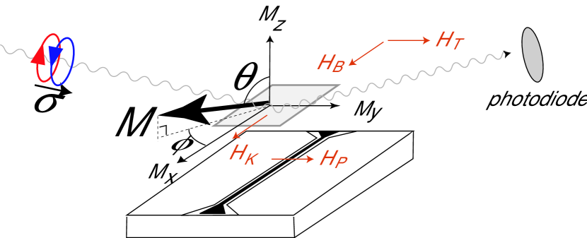
Figure 1: TR-XMCD measurement configuration. Circularly polarized photons are reflected at grazing incidence into a photodiode (right). XMCD is measured by switching photon helicity $\mathbf{\sigma}$. Relative alignment of applied fields $H_{P}$ (pulse), $H_{B}$ (longitudinal bias), $H_{K}$ (anisotropy), and $H_{T}$ (transverse bias) is shown.

We present direct experimental separation of Ni and Fe magnetic moment precession in ferromagnetic Ni₈₁Fe₁₉(50nm) through pump-probe XMCD. Improved time resolution ($\sim\textrm{90 ps}$ FWHM) has been achieved in part through the use of a fast-falltime squarewave magnetic field pulse delivered through a coplanar waveguide (CPW).Kos et al. (2002) We verify coupled precession of elemental moments within instrumental resolution.

II Experimental

Time-resolved XMCD (TR-XMCD) measurements were carried out at Beamline 4-ID-C of the Advanced Photon Source in Argonne, IL. The circular dichroism signal was obtained in reflectivity at near grazing incidence (see Fig 1), using photon helicity $\mathbf{\sigma}$ switching ($\mathbf{\sigma}\parallel\mathbf{\hat{y}}$) at the elliptical undulator for fixed applied field $\mathbf{H}$. Reflected intensity was read at a soft x-ray photodiode and normalized to an incident intensity at a reference grid. The measurement technique is photon-in/photon out and should therefore minimize artifacts from time-varying stray magnetic fields.

Time resolution was achieved through a pump-probe technique. Fast fall-time magnetic field pulses (pump) were synchronized with variable delay to x-ray photon bunches from the APS storage ring (probe.) The repetition frequencies of photon bunches and magnetic field pulses were both 88.0 MHz (11.37 ns period); therefore, source or detector gating was not required.

The magnetic field delivery configuration is similar to that used in a pulsed inductive microwave permeameter (PIMM). Kos et al. (2002); Reidy et al. (2003). Fast fall-time current pulses ($\sim$ 150ps) were delivered from a commercial pulse generator and through a CPW located under the magnetic thin film, providing pulsed transverse fields $<$ 10 Oe in amplitude. Pulses terminated into a 20 GHz sampling oscilloscope with 27 dB attenuation for pulse waveform characterization or directly into a 50$\Omega$ load during TR-XMCD measurement. The CPW center conductor was aligned along $\mathbf{\hat{x}}$, generating pulse fields $\mathbf{H_{P}}=H_{P}\>\mathbf{\hat{y}}$. Orthogonal Helmholtz coils apply longitudinal bias $\mathbf{H_{B}}=H_{B}\>\mathbf{\hat{x}}$ or transverse magnetic field bias $\mathbf{H_{T}}=H_{T}\>\mathbf{\hat{y}}$.

Experimental system time resolution can be estimated by using the finite photon bunch length $\sigma_{ph}$ and the timing jitter in the current pulse delivery electronics $\sigma_{tj}$. Separate streak camera measurements provide RMS bunch length $\sigma_{ph}=\textrm{25 ps}$A. Lumpkin and sampling oscilloscope measurements provide RMS timing jitter $\sigma_{tj}=\textrm{30 ps}$. Adding these contributions in quadrature yields a net timing resolution of $\sqrt{\sigma_{ph}^{2}+\sigma_{tj}^{2}}=\textrm{39 ps}$ RMS or 90 ps FWHM.

The Ni₈₁Fe₁₉(50nm)/Ta(2nm) thin film was deposited on the CPW using ion beam sputtering at a base pressure of 5$\times$10^-8 Torr. Magnetic anisotropy was induced using a static magnetic field applied along the center conductor, creating an effective uniaxial anisotropy field $\mathbf{H_{K}}\parallel\mathbf{\hat{x}}$. The sample normal points along $\mathbf{\hat{z}}$; the plane of incidence of the beam is $yz$, oriented roughly 5^∘ off $\mathbf{y}$. During TR-XMCD, magnetization was longitudinally biased, $\textrm{0}<H_{B}<\textrm{100 Oe}$, along the easy anisotropy axis, therefore $\mathbf{M}\bot\mathbf{\sigma}$, and magnetization was rotated over small angles by the pulsed oersted field $H_{P}\sim 7\>\mathbf{Oe}$. Measurements were carried out at room temperature (295 K).

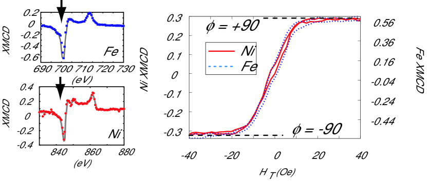
Figure 2: Left: XMCD spectra over L₃ and L₂ edges for Ni and Fe. Photon energy was set to the $L_{3}$ peak for Ni and Fe before measurement of element-specific hysteresis loops (right.). The signal provides a calibration for the elemental magnetization angles $\phi_{Ni}$ and $\phi_{Fe}$.

Element-specific XMCD hysteresis loops were taken as a function of transverse bias $H_{T}$ to obtain a calibration for rotation angle $\phi$ (Fig 2.) Photon energies were set to the L₃ peaks for Fe (701 eV) and Ni (844eV) to measure Fe and Ni XMCD signals respectively (Fig 2, left;) nominal energies were close to reported peak energies of 707 eV and 853 eV, respectively. The saturation values of XMCD signals are taken to be $\phi_{Ni}=\phi_{Fe}=\pm\textrm{90}^{\circ}$. Well-defined hard-axis loop behavior is shown with an anisotropy field $H_{K}$ of 11.8 $\pm$ 1.0 Oe (Fig 2, right); the Fe dichroism signal is roughly a factor of two larger than the Ni dichroism signal, consistent with previous workEriksson et al. (1990) and the smaller number of holes in Ni.

III Results

The measurement of magnetization precession for Ni moments alone is presented in Figure 3. XMCD signals were measured as a function of pump-probe delay and converted to time-dependent elemental Ni magnetization angles $\phi_{Ni}(t)$ according to Fig 2. Damped precessional oscillations are clearly seen, diminishing in amplitude (20^∘ to 5^∘) and increasing in frequency (1.6 to 2.6 GHz) with increasing longitudinal bias $0<H_{B}<100\>\textrm{Oe}$.

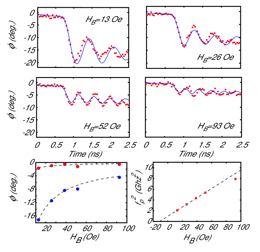
Figure 3: Time-dependence of Ni magnetization angle $\phi_{Ni}(t)$ after falling magnetic field (points), with LLG simulation (lines). Top left: H_B=13 Oe. Top right: H_B=26 Oe. Middle left: H_B=52 Oe. Middle right: H_B=93 Oe. Bottom left: equilibrium magnetization angles for high and low pulse levels; bottom right: Kittel plot of extracted precessional frequencies.

Single-domain Landau-Lifshitz-Gilbert (LLG) simulations of Ni magnetization dynamics are plotted with the experimental data. Consistent parameters are used for the fits. These are M_s=830 kA/m, measured by SQUID and $g_{eff}=2.05$, extracted from previous PIMM measurement. The anisotropy field H_K=11.4$\pm$0.5 Oe, determined according to the Kittel relationship $\omega_{p}^{2}=\gamma^{2}\mu_{0}^{2}M_{s}H_{\parallel}$ for in-plane magnetization precession and plotted in the right bottom panel of Figure 3, agrees within experimental error with that measured statically by element-resolved hysteresis loops (Fig. 2, right.) The pulse field $H_{P}(t)$ was taken to be proportional to the transmitted current waveform $i_{pulse}(t)$ at the oscilloscope; scaling for the pulse was found by fitting the steady-state pre- and post-falling edge levels of magnetization angle $\phi_{Ni}(0.5)$ and $\phi_{Ni}(\textrm{4.5ns})$, respectively, yielding maximum pulse field level $H_{P}$=7.2 Oe.

The Fe magnetization angles have been processed similarly. Differences between high and low saturation angles for Fe and Ni TR-XMCD scans ($\Delta\phi_{Ni,Fe}$) are plotted in Figure 4 as a function of longitudinal bias $H_{B}$. Agreement between experimental $\Delta\phi_{Ni}(H_{B})$, experimental $\Delta\phi_{Fe}(H_{B})$, and the single-domain model is satisfactory after application of an 11% increase in the XMCD-to-$\phi$ calibration factor found from the Fe hysteresis loop (Fig. 2). This level of adjustment is close to the level of drift measured in the saturation level of the Fe loop. High saturation levels of Fe are then offset to match those of Ni, by values varying from 0-2^∘.

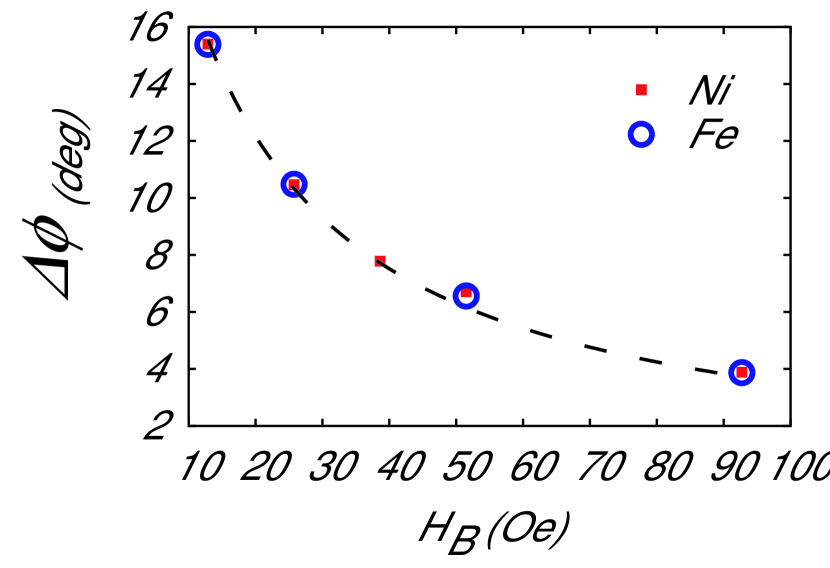
Figure 4: Differences between high and low saturation angles of the elemental Ni and Fe scans during TR-XMCD measurement, $\Delta\phi=\phi(\textrm{t=0.5ns})-\phi(\textrm{t=4.5ns})$. Measured points for Ni and Fe are shown with the single-domain model fit.

Element-specific precession is shown in Figure 5. Ni and Fe moments are shown to precess together within instrumental resolution ($\pm$45 ps). As the longitudinal bias field $H_{B}$ increases, the precessional frequency increases for both elements and there is no apparent development of a phase lag greater than experimental error.

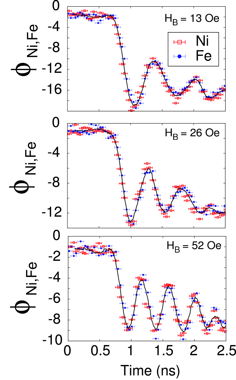
Figure 5: TR-XMCD measurement of Fe and Ni magnetization angle during free precession. Top: $H_{B}=\textrm{13 Oe}.$ Middle: $H_{B}=\textrm{26 Oe}.$ Bottom: $H_{B}=\textrm{52 Oe}.$ Lines are a polynomial smoothing function applied to both data sets; timing errors of $\pm$ 45 ps are indicated.

IV Discussion

Ni and Fe magnetic moment precession is observed to be coupled in phase, within 90 ps, during FMR precession of Ni₈₁Fe₁₉. The measurement provides direct experimental confirmation that the net Fe and Ni elemental moments are collinear during precession at time scales exceeding 90 ps. It should be noted that this result could not have been easily determined without assumption from existing measurement techniques such as PIMM or time-resolved magnetooptical Kerr effect.

The result indicates that the exchange force exceeds the tendency of moments on Ni and Fe to precess or relax at different rates. The time resolution of the experiment is on the order of the spin-lattice relaxation time $\tau_{sl}$ characterized for GdVaterlaus et al. (1991), 100 $\pm$ 80 ps, which characterizes the direct spin-to-lattice relaxation channel; these values are unknown for transition metals but can be expected to be within an order of magnitude. A tendency for Fe and Ni moments to relax at different rates is plausible based on the orbital to spin moment ratios $L/S$ of Ni and Fe characterized in Ni₈₁Fe₁₉ by XMCD, 0.12 and 0.08 respectively.Foy et al. (2003)

The prospect of partially-coupled motion is more likely in systems where exchange coupling is weaker and/or magnetic moments are more localized. Transition-metal - rare-earth alloys, featuring lower Curie temperatures and more isolated $f$-shells on the rare-earths, would be attractive systems to study using the technique. Many rare-earth dopants in Ni₈₁Fe₁₉ have been found to increase the FMR lossReidy et al. (2003), and TR-XMCD can test the possibility that some loss is carried by a phase lag between RE and TM moments.Clarke et al. (1965) Similarly, the trilayer structures used in spin electronics (e.g. NiFe/Cu/CoFe) offer the possibility of continuous adjustment of interlayer coupling through the spacer thickness.

Finally, we note the possibility of additional studies through more detailed spectroscopic information. Spin and orbital moment dynamics may be separated on individual elements through the use of sum rules. We take the point time resolution as that of the measurement; it should be noted that edge resolution, with long enough averaging and continuous monitoring for drift of the pulse amplitude $H_{P}$, could be improved. Better control over pulse delivery jitter will allow a point resolution limited only by $\sigma_{ph}$ and longer averaging could allow edge resolution better than that of the lower bound of $\tau_{sl}$.

V Conclusion

We have separated Ni and Fe moment motion in Ni₈₁Fe₁₉ by TR-XMCD, demonstrating elemental resolution in ferromagnetic resonance up to 2.6 GHz. Coupled motion of elemental moments is found to a time resolution of $\pm$ 45 ps and an angular resolution better than 2^∘.

VI Acknowledgements

We thank Gary Nitzel (NSLS) for technical support. This work was partially supported by the Army Research Office, grant ARO-43986-MS-YIP. Use of the Advanced Photon Source was supported by the U. S. Department of Energy, Office of Science, Office of Basic Energy Sciences, under Contract No. W-31-109-Eng-38. Research was carried out in part at the National Synchrotron Light Source, Brookhaven National Laboratory, which is supported by the U.S. Department of Energy, Division of Materials Sciences and Division of Chemical Sciences, under Contract No. DE-AC02-98CH10886.

References

- Malajovich et al. (2000) I. Malajovich, J. Kikkawa, D. Awschalom, J. Berry, and N. Samarth, Physical Review Letters 84, 1015 (2000).
- Marohn et al. (1995) J. Marohn, P. Carson, J. Hwang, M. Miller, D. Shykind, and D. Weitekamp, Physical Review Letters 75, 1364 (1995).
- van Schilfgaarde et al. (1999) M. van Schilfgaarde, I. Abrikosov, and B. Johansson, Nature 400, 46 (1999).
- Mikke et al. (1977) K. Mikke, J. Jakowska, Z. Osetek, and A. Modrzejewski, J. Phys. F.: Metal Phys. 7, L211 (1977).
- (5) private communication, T. Schulthess.
- Foy et al. (2003) E. Foy, S. Andrieu, M. Finazzi, R. Poinsot, C. Teodorescu, F. Chevrier, and G. Krill, Physical Review B (Condensed Matter and Materials Physics) 68, 94414 (2003).
- Farle (1998) M. Farle, Reports on Progress in Physics 61, 755 (1998).
- Chen et al. (1995) C. Chen, Y. Idzerda, H.-J. Lin, N. Smith, G. Meigs, E. Chaban, G. Ho, E. Pellegrin, and F. Sette, Physical Review Letters 75, 152 (1995).
- Bonfirm et al. (2001) M. Bonfirm, G. Ghiringhelli, F. Montaigne, S. Pizzini, N. Brookes, F. Petroff, J. Vogel, J. Camarero, and A. Fontaine, Physical Review Letters 86, 3646 (2001).
- Kos et al. (2002) A. Kos, T. Silva, and P. Kabos, Review of Scientific Instruments 73, 3563 (2002).
- Reidy et al. (2003) S. Reidy, L. Cheng, and W. Bailey, Applied Physics Letters 82, 1254 (2003).
- (12) private communication, A. Lumpkin, Advanced Photon Source,Feb. 2004,.
- Eriksson et al. (1990) O. Eriksson, B. Johansson, R. Albers, A. Boring, and M. Brooks, Physical Review B (Condensed Matter) 42, 2707 (1990).
- Vaterlaus et al. (1991) A. Vaterlaus, T. Beutler, and F. Meier, Physical Review Letters 67, 3314 (1991).
- Clarke et al. (1965) B. Clarke, K. Tweedale, and R. Teale, Physical Review 139, A1933 (1965).