Thermopower in Andreev Interferometers

Abstract

We examine the thermopower $Q$ of a mesoscopic normal-metal (N) wire in contact to superconducting (S) segments and show that even with electron-hole symmetry, $Q$ may become finite due to the presence of supercurrents. Moreover, we show how the dominant part of $Q$ can be directly related to the equilibrium supercurrents in the structure. We also discuss the thermopower arising due to an anomalous kinetic coefficient which is finite in the presence of supercurrent and in some situations gives the dominant contribution. In general, a finite thermopower appears both between the N reservoirs and the superconductors, and between the N reservoirs themselves. The latter, however, strongly depends on the geometrical symmetry of the structure. The paper includes a detailed analytical derivation of the results and an exact numerical solution of the quasiclassical equations in a few sample geometries.

PACS numbers: 74.25.Fy, 73.23.-b, 74.45.+c

1 INTRODUCTION

From time to time in the last century, the connection between the thermoelectric effects and superconductivity has attracted interest.[1] As early as 1927, Meissner found that the thermopower is absent in a steady-state superconductor. This is due to the fact that the thermoelectric current is in this case counterbalanced by the supercurrent. However, in 1944, Ginzburg [2] pointed out that there can be other types of thermoelectric effects in superconductors. Interestingly, many of them are still unobserved [1], at least partially due to the fact that they are based on the same electron-hole asymmetry that produces the thermoelectric effects in nonsuperconducting systems [3], where Mott’s law connects the thermopower to the tiny difference of the effective masses between electrons and holes (i.e., to the nonlinearity of the quasiparticle dispersion relation above and below the Fermi sea). Such effects are governed by the factor $k_{B}T/E_{F}$, and are thus very small in the low temperatures required for superconductivity. Even after six decades, the understanding of the experiments on some of these effects is still lacking.[4, 5] For example, the measured thermoelectric flux in a bimetallic superconducting ring was orders of magnitude larger than predicted by the conventional theories.

Another effect of thermoelectric type, finite even in the presence of complete electron-hole symmetry, was observed and successfully explained in the turn of 1980’s:[6, 7, 8, 9] it was found that the combination of a temperature gradient and supercurrent could make rise to a charge (branch) imbalance, i.e., a difference in the electrochemical potentials of the normal and superconducting components. The origin of this effect is similar to that considered in this paper, but it manifests itself in quite a different form in the systems studied here.

In the 1990’s, many groups started to investigate the superconducting effects induced in normal-metal (N) wires from nearby superconductors (for review, see Refs. raimondilambert,courtoispannetier,belzig99). For example, if the N metal is connected to two superconducting segments, one can drive a supercurrent through it [13]. It was found that this superconducting proximity effect influences both the electrical [14, 15] and thermal [16] conductances of the N wire, in general breaking the Wiedemann-Franz relation between the two.[17] In most cases, these effects account for some tens of percent changes in the conductances.

In proportion, a much greater effect was experimentally observed in the thermopower [18, 19, 20, 21, 22] of "Andreev interferometers", structures where the normal-metal wire was connected to two ends of a broken superconducting loop. The observed thermopower was found to be orders of magnitude larger with the proximity effect (below the superconducting critical temperature $T_{C}$) than without it ($T>T_{C}$). A thermally induced voltage was found both between the ends of the normal metal [18, 19, 20, 22] ("N-N thermopower" $Q_{NN}$) as also between one end of the normal metal and the superconducting contacts ("N-S thermopower" $Q_{NS}$).[21, 22] Moreover, it was found that this induced thermopower oscillates with the flux applied through the superconducting loop.

It was shown in Ref. heikkila00, including one of the present authors, that Mott’s law is not in general valid in the presence of the proximity effect, indicating that the reason underlying the observations is not necessarily dependent on electron-hole symmetry. Indeed, the experimental observations were partially explained, without invoking electron-hole asymmetry, in the linear regime for $Q_{NS}$ by Seviour and Volkov [24] and another effect was suggested for the presence of $Q_{NN}$ by Kogan, Pavlovskii and Volkov.[25] The full nonlinear regime, including important effects coming from asymmetries in the structure, and a phenomenological explanation that connects the thermopower to the temperature dependence of the supercurrent, was described by the present authors in Ref. virtanen04. This theory seems to be in quantitative and qualitative agreement with most of the observations. The aim of the present paper is to explain this theory in detail and describe a related effect, thermopower due to an anomalous kinetic coefficient, which is the main source of thermopower in certain geometries.

Further, Ref. heikkila03 shows that the presence of supercurrent can lead also to a Peltier-type effect. This effect has not yet been experimentally observed.

This paper is organized as follows. In Sect. 2, we detail the quasiclassical formalism applied in the calculation of the thermopower. This formalism assumes complete electron-hole symmetry, and the predicted effects are hence not limited by the factor $k_{B}T/E_{F}$. The analytic approximations necessary for obtaining an expression for the thermopower are presented in Sect. 3, including symmetry arguments for the full (without approximations) solutions, a phenomenological picture of the effect, and a calculation of the thermopower in the quasiequilibrium limit. The general behavior of this thermopower is detailed in Sect. 4, and effects related to the geometry of the studied structures are discussed in Sect. 5 Most of the results in these sections are obtained numerically without any approximations (beyond the quasiclassical diffusive limit). Section 6 includes a comparison of the theory to the experiments and to the other theories on the effect. The main spectral coefficients responsible for the thermopower, the spectral supercurrent and the anomalous coefficient $\mathcal{T}$, are described in Sect. 7 Finally, the results are shortly discussed in Sect. 8 An impatient reader should capture mostly the kinetic equations (7) in Sect. 2, skip the detailed analytic derivations in Subs. 3.5 and proceed with the main results in Subs. 3.6 and their characteristics in Secs. 4,5

2 FORMALISM

Many well-understood phenomena in inhomogeneous superconductivity have been explained through the use of quasiclassical Green’s functions. This is in particular the case in mesoscopic superconductivity (see the reviews in Refs. raimondilambert,belzig99). The essence of the quasiclassical theory is ignoring the short-scale oscillations in the relative coordinate, and concentrating only on the center-of-mass coordinate of the space-dependent Green’s functions. Such an approximation ignores the quantum-mechanical interference effects arising from short scales of the order of the Fermi wavelength (structural variations on this scale can be included through boundary conditions, see below and Ref. nazarov99), and the effects related to the nonlinear parts of the quasiparticle dispersion relation (the theory is based on the linearisation of the dispersion relation around the Fermi energy). Therefore, it cannot describe the normal-metal thermoelectric effects which arise from the energy dependence of the effective mass.

In this paper, we concentrate on the diffusive limit, where all the important length scales are much greater than the mean free path. This is typically the case in metallic wires. To describe nonequilibrium effects (finite voltage) in the nonlinear regime, we adopt the Keldysh formalism.[29] In the considered limit, the Keldysh–Green’s function is described by the Usadel equation.[30]

2.1 Keldysh–Usadel equations

The Keldysh–Usadel equation for the Green’s functions $\check{G}(\vec{r},E)$ in the Keldysh $\otimes$ Nambu space can be written in the static case as

$$\nabla\cdot(D\check{G}\nabla\check{G})=\left[-iE\;1\otimes\hat{\tau}_{3}+\check{\Delta}+\check{\Sigma}_{\text{in}},\check{G}\right]\,.$$ (1)

Here, $D$ is the diffusion constant of the metal, $\check{\Sigma}_{\text{in}}$ contains the inelastic scattering self-energies, and $\check{\Delta}$ is the pair potential matrix. The pair potential is self-consistently related to the solutions of Eq. (1), [12] but it vanishes in normal metals, on which we concentrate here (superconductivity is induced by a boundary condition from bulk superconductors). Moreover, $\check{G}$ has the matrix structure

$$\check{G}=\begin{pmatrix}\hat{G}^{R}&\hat{G}^{K}\\ 0&\hat{G}^{A}\end{pmatrix}\,,\;\hat{G}^{A}=-\hat{\tau}_{3}(\hat{G}^{R})^{\dagger}\hat{\tau}_{3}\,,\;\hat{G}^{K}=\hat{G}^{R}\hat{h}-\hat{h}\hat{G}^{A}\,,$$ (2)

where $\hat{G}^{R}$, $\hat{G}^{A}$ and $\hat{G}^{K}$, the retarded, advanced and Keldysh components, are $2\times 2$ matrices, and the last relation is due to the normalization $\check{G}^{2}=\check{1}$. The electron–hole distribution function matrix $\hat{h}$ introduced here has two free parameters and it can be chosen of the form $\hat{h}\equiv f_{L}\hat{1}+f_{T}\hat{\tau}_{3}$, where $f_{T}$ and $f_{L}$ are the symmetric and antisymmetric parts,

$$f_{T}(E)\equiv 1-\mathfrak{f}(\mu_{S}-E)-\mathfrak{f}(\mu_{S}+E),\;f_{L}(E)\equiv\mathfrak{f}(\mu_{S}-E)-\mathfrak{f}(\mu_{S}+E)\,$$ (3)

of the electron distribution function $\mathfrak{f}(\vec{r},E)$ and the energy $E$ is given with respect to the potential $\mu_{S}$ of the superconductors.

The Green’s function obtained from Eq. (1) may be used for evaluating the observable energy and charge current densities $j_{Q}$ and $j_{c}$:

$$j_{Q} =\frac{\sigma}{2e^{2}}\int\!Ej_{L}\,\mathrm{d}E\,, j_{c} =\frac{\sigma}{2e}\int\!j_{T}\,\mathrm{d}E\,,$$ (4a)

$$j_{L} \equiv\frac{1}{4}\text{Tr}[(\tau_{1}\otimes\hat{1})\,\check{G}\nabla\check{G}\,]\,, j_{T} \equiv\frac{1}{4}\text{Tr}[(\tau_{1}\otimes\hat{\tau}_{3})\,\check{G}\nabla\check{G}\,]\,.$$ (4b)

Here, $j_{L}$ and $j_{T}$ are the spectral current densities, and $\sigma$ is the normal-state conductivity of the metal.

It is useful to parameterize $\check{G}$ so that it automatically satisfies the normalization. Since $\check{G}^{2}=\check{1}$ implies that $(\hat{G}^{R})^{2}=\hat{1}$, one can parametrize $\hat{G}^{R}$ in terms of two complex functions $\theta$ and $\chi$ as

$$\hat{G}^{R}=\begin{pmatrix}\cosh(\theta)&e^{i\chi}\sinh(\theta)\\ -e^{-i\chi}\sinh(\theta)&-\cosh(\theta)\end{pmatrix}\,,$$ (5)

and hence $\hat{G}^{A}$ and $\hat{G}^{K}$ depend only on $\theta$, $\chi$, $f_{T}$ and $f_{L}$. To find the equations that determine $\theta$ and $\chi$, one can consider the retarded part in Eq. (1), and, neglecting inelastic effects ($\check{\Sigma}_{\text{in}}=0$), obtain the spectral Keldysh–Usadel equations in normal metals ($\check{\Delta}=0$)

$$D\nabla^{2}\theta=-2iE\sinh(\theta)+\frac{1}{2}D(\nabla\chi)^{2}\sinh(2\theta)\,,$$ (6a)

$$D\nabla\cdot j_{E}=0,\quad j_{E}\equiv-\sinh^{2}(\theta)\nabla\chi\,.$$ (6b)

These equations describe the behavior of the superconducting proximity effect: the pairing amplitude can be written as $F=\sinh(\theta)\exp(i\chi)$, which shows that $\theta$ is related to the strength of the proximity effect and $\chi$ to the phase of the superconducting order parameter.

Using the same assumptions as above and taking the traces $\text{Tr}[(\tau_{1}\otimes\hat{1})\;\cdot\;]$ and $\text{Tr}[(\tau_{1}\otimes\hat{\tau}_{3})\;\cdot\;]$ of Eq. (1), one obtains the kinetic equations for the spectral energy and charge current densities

$$D\nabla\cdot j_{L} =0, j_{L}=\mathcal{D}_{L}\nabla f_{L}-\mathcal{T}\nabla f_{T}+j_{S}f_{T}\,,$$ (7a)

$$D\nabla\cdot j_{T} =0, j_{T}=\mathcal{D}_{T}\nabla f_{T}+\mathcal{T}\nabla f_{L}+j_{S}f_{L}\,.$$ (7b)

These describe the kinetics of electrons and holes in the presence of the proximity effect, and, moreover, imply that $j_{L}$ and $j_{T}$ are conserved. The spectral coefficients in Eqs. (7) are determined from the solutions to Eqs. (6):

$$\mathcal{D}_{L} \equiv\frac{1}{4}\text{Tr}[1\!-\!\hat{G}^{R}\hat{G}^{A}]=\frac{1}{2}(1+|\cosh\theta|^{2}-|\sinh\theta|^{2}\cosh(2\text{Im}[\chi])),$$ (8a)

$$\mathcal{D}_{T} \equiv\frac{1}{4}\text{Tr}[1\!-\!\hat{G}^{R}\hat{\tau}_{3}\hat{G}^{A}\hat{\tau}_{3}]=\frac{1}{2}(1+|\cosh\theta|^{2}+|\sinh\theta|^{2}\cosh(2\text{Im}[\chi])),$$ (8b)

$$\mathcal{T} \equiv\frac{1}{4}\text{Tr}[\hat{G}^{A}\hat{G}^{R}\hat{\tau}_{3}]=\frac{1}{2}|\sinh\theta|^{2}\sinh(2\text{Im}[\chi])),$$ (8c)

$$j_{S} \equiv\frac{1}{4}\text{Tr}[(\hat{G}^{R}\nabla\hat{G}^{R}-\hat{G}^{A}\nabla\hat{G}^{A})\hat{\tau}_{3}]=\text{Im}[-\sinh^{2}(\theta)\nabla\chi]=\text{Im}[j_{E}].$$ (8d)

Here, $\mathcal{D}_{L}$ and $\mathcal{D}_{T}$ are the spectral energy and charge diffusion coefficients, and $j_{S}$ is the spectral density of the supercurrent-carrying states. [31] The cross-term $\mathcal{T}$ is usually small but not completely negligible.

To simplify the problem, one often assumes that wires are quasi-1D structures, i.e., much longer than wide, and translationally invariant in their latitudinal directions. Thus, one needs only to consider longitudinal variation in the quantities, and the gradients may be replaced with 1D-derivatives.

2.2 Boundary conditions

The Keldysh–Usadel equations cannot handle changes in the structure which occur in a distance short compared to the Fermi wavelength or the mean free path, so boundary conditions describing interfaces and junctions need to be derived using different techniques.

To obtain the boundary conditions at nodes of one-dimensional wires with clean metallic contacts, one may use the the matrix circuit theory. [28] It yields a Kirchhoff-like conservation law for the spectral matrix currents $A\sigma\check{G}\partial_{x}\check{G}$, where $A$ is the cross-sectional area of a wire. In the $\theta$-parameterized form, this results in

$$\sum_{i}A_{i}\sigma_{i}\nabla\theta_{i} =0, \sum_{i}A_{i}\sigma_{i}\nabla\chi_{i} =0,$$ (9a)

$$\sum_{i}A_{i}\sigma_{i}j_{L} =0, \sum_{i}A_{i}\sigma_{i}j_{T} =0,$$ (9b)

and to the continuity of $\theta$, $\chi$, $f_{L}$ and $f_{T}$. In Eqs. (9), the sums go over the wires ending in the node.

The properties of connections between wires and terminals are also described by a matrix conservation condition. [28] In the limit of a clean metallic contact, at the interface to a normal reservoir, Green’s function $\check{G}$ and thus also $\theta$, $\chi$, $f_{L}$ and $f_{T}$ get their bulk values:

$$\theta =0,\quad\chi=\textrm{arbitrary},$$ (10a)

$$f_{L/T} =\frac{1}{2}\left(\tanh\left(\frac{E+\mu}{2k_{B}T}\right)\pm\tanh\left(\frac{E-\mu}{2k_{B}T}\right)\right),$$ (10b)

where $T$ is the temperature of the reservoir and $\mu$ its potential, compared to $\mu_{S}$. Thus, near normal metal reservoirs or far from superconductors, the coefficients (8) obtain their normal-state bulk values $\mathcal{D}_{L}\rightarrow 1$, $\mathcal{D}_{T}\rightarrow 1$ and $\mathcal{T}\rightarrow 0$.

At a clean metallic contact to a superconducting reservoir, bulk values are again obtained, with the exception of $f_{L}$ for energies inside the superconducting energy gap $\Delta$:

$$\theta=\textrm{artanh}\frac{\Delta}{E},\quad\chi=\phi,\quad f_{T}=0,$$ (11a)

$$|E|>\Delta:\quad f_{L}=\tanh\left(\frac{E}{2k_{B}T}\right),$$ (11b)

$$|E|<\Delta:\quad j_{L}=0\,.$$ (11c)

Here, $\phi$ is the phase of the superconducting order parameter. We assumed here no charge imbalance, $\mu_{S}=0$, hence $f_{T}=0$. Moreover, the boundary conditions for $\theta$ and $\chi$ imply that near a superconductor interface $\mathcal{D}_{L}\rightarrow 0$ and $\mathcal{T}\rightarrow 0$ for energies $|E|<\Delta$, which in fact implies that $j_{L}=0$. Thus no contribution to the energy current density $j_{Q}$ through the interface comes from inside the energy gap — this is a known property of the Andreev reflection.

With these boundary conditions, the spectral equations (6) depend only on the phase differences and the geometry of the system, while kinetic equations (7) depend also on the temperatures and the potentials of the reservoirs. The system is, however, fully decoupled from the temperatures of the superconductors for the energies $|E|<\Delta$.

Note that in wires connected to a normal reservoir, the spectral supercurrent $j_{E}\equiv 0$, due to the boundary condition $\theta=0$. Since generally $\sinh(\theta)\not\equiv 0$ in these wires, the conservation of spectral supercurrent $j_{S}$ implies the conservation of the phase, thus $\chi=\textrm{const}(x)$. Similarly, in wires connected to a superconducting reservoir, there is the boundary condition $j_{L}\equiv 0$ for $|E|<\Delta$, and one can eliminate $f_{L}$ from the kinetic equations.

2.3 Energy and length scales

Scaling the spatial dimensions in the spectral equations (6) by the length $L$ (where $L$ can be one of the wire lengths, or most naturally for the supercurrent, the distance between the superconductors), one finds a natural energy scale: the Thouless energy

$$E_{T}\equiv\frac{\hbar D}{L^{2}}\approx\left\{\begin{array}[]{cc}13\leavevmode\nobreak\ \mu\text{V}&\;e\\ 0.15\leavevmode\nobreak\ \text{K}&\;k_{B}\end{array}\right\}\;\frac{D/(200\leavevmode\nobreak\ \mathrm{\frac{cm^{2}}{s}})}{(L/\mathrm{\mu{}m})^{2}}\,,$$ (12)

This energy is the inverse time of flight through a diffusive wire of length $L$.

In practice, there are two different types of energy scales describing the behavior of the spectral functions: $E_{T}$ and the superconducting energy gap $\Delta$ of the electrodes connected to the normal-metal wire. [31] The previous is important in the case of long junctions $L\gg\xi_{0}$ (i.e., $E_{T}\ll\Delta$) and the latter for $L\lesssim\xi_{0}$ ($E_{T}\gtrsim\Delta$). Here $\xi_{0}=\sqrt{\hbar D/2\Delta}$ is the superconducting coherence length. For example, for $T\ll T_{C}$, in Al $\xi_{0}\approx 200$ nm, and in Nb $\xi_{0}\approx 30$ nm.

In the long-junction limit $\Delta\gg E_{T}$, the energy scale for the solution to (6,7) with the boundary conditions (9-11) depends only on $E_{T}$. Thus, by changing $E_{T}$, the results may be scaled to fit all systems with similar ratios of wire lengths, cross sectional areas and conductivities.

3 THERMOPOWER IN ANDREEV INTERFEROMETERS

A temperature difference $\Delta T$ between two points in a metal may induce a charge current $I_{c}$. Disconnecting the system from its surroundings makes the current vanish, and a potential difference $\Delta V$ arises instead. The thermopower $Q$ is the ratio of this potential difference to the temperature difference, $Q\equiv\left(\Delta\!V/\Delta\!T\right)_{I_{c}=0}$. In this section, we show how the supercurrent flowing in Andreev interferometers connects the temperatures and potentials, inducing a finite thermopower.

3.1 Thermopower without superconductivity

An estimate for the thermopower in the absence of superconductivity can be found using the semiclassical Boltzmann equation as, for example, in Ref. ashcroft. Such a description can be obtained from the microscopic theory presented above, provided that the length scales important for the problem are much greater than the Fermi wavelength.[29] This analysis leads to the Mott relation for the thermopower

$$Q=-\frac{\pi^{2}}{3}\,\frac{k_{B}^{2}T}{e}\,\left.\frac{\mathrm{d}\ln{\sigma(E)}}{\mathrm{d}E}\right|_{E=E_{F}}\,.$$ (13)

Here, $\sigma(E)$ describes a generalized conductivity — $\sigma(E_{F})$ gives the actual conductivity in the linear-response regime — and the logarithmic derivative depends on the energy dependence of the elastic relaxation time and the exact structure of the Fermi surface. The previous can typically be neglected, and the latter is due to the small asymmetry between the dispersion relations for electrons and holes. Both of these effects are neglected in the quasiclassical theory. There are also other major contributions to the thermopower, e.g. the phonon drag, but for simple metals, they should vanish at high and very low temperatures. [32]

We can use the temperature dependence in Eq. (13) for an extrapolation from the room-temperature values of $Q$ to its value at subkelvin temperatures. Usual magnitudes for the thermopower at the room temperature are of the order $\mathrm{\frac{\mu{}V}{K}}$ for pure metals. To obtain a rough estimate at a low temperature, we extrapolate $10\leavevmode\nobreak\ \mathrm{\frac{\mu{}V}{K}}$ from room temperature to a temperature of 0.5 K (typical for the studies on the proximity effect), which yields $Q\sim 10\leavevmode\nobreak\ \mathrm{\frac{nV}{K}}$. Measurements in Ref. parsons03 gave a stricter estimate $Q\lesssim 1\leavevmode\nobreak\ \mathrm{\frac{nV}{K}}$ for their case.

However, the Keldysh–Usadel equations predict the presence of a large thermopower $Q\sim\mathrm{\frac{\mu{}V}{K}}$, even under complete electron-hole symmetry, as supercurrents couple the temperatures to the potentials (through the coefficients $j_{S}$ and $\mathcal{T}$ in the kinetic equations (7)).

3.2 Modeled structure

Figure 1: The system under examination. The terminals S are superconducting reservoirs, N normal-metal reservoirs and they are connected by normal-metal wires with lengths $L_{k}$, cross sections $A_{k}$ and normal-state conductivities $\sigma_{k}$, $k=1\ldots 5$. Temperatures $T$ and potentials $\mu=eV$ in the reservoirs are as shown. Moreover, all contacts are assumed clean metallic. Positive directions for currents are indicated with arrows.

Here we focus to study thermopower in the structure shown in Fig. 1, where two superconducting (S) reservoirs with a phase difference $\phi$ are connected through a normal-metal link to two normal metal (N) reservoirs. When measuring thermopower in this structure, no current flows in wires 1 and 2,

$$j_{c,1}=0,\quad j_{c,2}=0,$$ (14)

and definite voltages $V_{1}$ and $V_{2}$ are induced in the N reservoirs. Here we may define several thermopower-like quantities:

$$Q_{\mathrm{NN}}=\frac{V_{2}-V_{1}}{T_{2}-T_{1}}\,,\quad{Q_{\mathrm{NS,1}}}=\frac{V_{1}}{T_{2}-T_{1}}\,,\quad{Q_{\mathrm{NS,2}}}=\frac{V_{2}}{T_{2}-T_{1}}\,.$$ (15)

Clearly, their behavior with varying parameters need not be similar. That is, generally the potential induced in the colder electrode may differ from that induced to the hotter electrode.

The thermopower appearing in the structure may be estimated by applying the formalism described in Sect. 2 We have solved Eqs. (6,7) numerically, and derived analytic approximations for the solutions of the kinetic equations (7). In the following, we first discuss the analytic results, as they provide some insight to the problem, and then examine interesting features numerically (Secs. 4 and 5).

3.3 Qualitative picture

The effect of supercurrents on the thermopower can be understood phenomenologically as follows. If $T_{1}\neq T_{2}$, the temperature-dependent [13] equilibrium supercurrent $I_{S}(T_{1})$ in wire 3 is different from $I_{S}(T_{2})$ in wire 4. (For this qualitative picture, we approximate these wires to be at the temperatures $T_{1}$, $T_{2}$ of the normal reservoirs.) Conservation of currents should still be maintained, so a compensating effect must arise. Should the normal reservoirs be kept at the same potential as the superconductors, a quasiparticle current $I_{\text{qp}}\propto(I_{S}(T_{1})-I_{S}(T_{2}))$ from them to the superconductors would balance the difference. However, when no current is allowed to flow in wires 1 and 2, a compensating N–S potential difference $V_{N}-V_{S}\propto R(I_{S}(T_{1})-I_{S}(T_{2}))$ is induced instead.

The qualitative picture gives the following predictions: First, the induced potentials should oscillate with the phase difference $\phi$ between the S electrodes, similarly to the supercurrent. Moreover, the potentials induced in the N electrodes need not be the same, especially if the resistances of the wires are not symmetric at the left and at the right. Thus, the supercurrent-effect also contributes, as in Eq. (31b), to the thermopower $Q_{\mathrm{NN}}$ between the N electrodes. Such a contribution should be present even in structurally symmetric setups, as the resistances are temperature-dependent due to the proximity effect. [14]

3.4 Phase behavior

If the phase difference between the superconducting elements vanishes, the quasiclassical equations predict a vanishing thermopower $Q$ (as shown below). In the presence of a phase difference, the supercurrent and the term $\mathcal{T}$ couple the two types of distribution functions, inducing a finite $Q$. Although the solution to Eq. (1) cannot be found in closed form, we can obtain information about the exact phase behavior of the thermopower using symmetry considerations. Suppose we have the solutions $\chi$, $\theta$, $f_{L}$ and $f_{T}$ for the Keldysh–Usadel equations (6,7) in the system. Then, define

$$\tilde{\chi}\equiv-\chi\,,\quad\tilde{\theta}\equiv\theta\,,\quad\tilde{f}_{L}\equiv f_{L}\,,\quad\tilde{f}_{T}\equiv-f_{T}\,.$$ (16)

First, we see that these new variables are solutions to Eqs. (6). This implies that $\tilde{\mathcal{D}}_{T}=\mathcal{D}_{T}$, $\tilde{\mathcal{D}}_{L}=\mathcal{D}_{L}$, $\tilde{\mathcal{T}}=-\mathcal{T}$ and $\tilde{j}_{S}=-j_{S}$, so the new variables are also solutions to Eqs. (7). They also satisfy the spectral current conservation (9), with $\tilde{j}_{T}=-j_{T}$ and $\tilde{j}_{L}=j_{L}$, and the boundary conditions (10,11), but with $\tilde{\phi}=-\phi$ and $\tilde{\mu}=-\mu$. Thus, there is a solution with inverted charge currents $I_{c}$, potentials $\mu$ and phases $\phi$. For the thermopower this implies that

$$Q(\phi)=\left.\frac{\Delta V}{\Delta T}\right|_{I_{c}=0}=-\left.\frac{\Delta\tilde{V}}{\Delta\tilde{T}}\right|_{\tilde{I}_{c}=0}=-Q(-\phi)\,.$$ (17)

Moreover, $Q$ is necessarily $2\pi$-periodic in phase, so this implies that it should also be antisymmetric with respect to $\phi=n\pi$ for all $n\in\mathbb{Z}$.

The result also implies that in a system with no phase differences or no superconducting parts, the thermopower vanishes. This is in agreement with the Mott-law prediction due to the quasiclassical approximation. However, note that the reasoning above assumes that the condition (14) determines the solution uniquely and that the thermopower is well defined. This may not be the case in some pathological geometries in the presence of the proximity effect, as the condition (14) is determined only for the energy-integrated currents. In the cases studied in the present manuscript, the convergence of numerics hints that the solutions are unique.

3.5 Analytic approximations

Although we cannot solve analytically the spectral equations in the structure of Fig. 1, we can obtain useful approximations starting from the kinetic equations.

As a first step, we assume that the induced potentials are small compared to the temperature, $|\mu|\ll k_{B}T$. Since $f_{T}$ is related to the potentials, we can reason that $f_{T}$ is small, and hence neglect the terms $-\mathcal{T}\partial_{x}f_{T}$ and $j_{S}f_{T}$ in Eq. (7a). Comparison with numerics shows that this is a good approximation.

The kinetic equations, where inelastic effects are neglected, can now be integrated over a wire of length $L$. This relates the currents to the distribution functions $f_{L}$, $f_{T}$ at the ends of the wire:

$$j_{L} =\frac{f_{L}(L)-f_{L}(0)}{L\bigl{<}\mathcal{D}_{L}^{-1}\bigr{>}}\,,$$ (18a)

$$j_{T} =\frac{f_{T}(L)-f_{T}(0)}{L\bigl{<}\mathcal{D}_{T}^{-1}\bigr{>}}+j_{S}f_{L}(0)$$ (18b)

$$+\frac{f_{L}(L)-f_{L}(0)}{L^{2}\bigl{<}\mathcal{D}_{L}^{-1}\bigr{>}\bigl{<}\mathcal{D}_{T}^{-1}\bigr{>}}\!\left(\int_{{0}}^{L}\!\!\!\!\frac{\mathcal{T}}{\mathcal{D}_{L}\mathcal{D}_{T}}\,\mathrm{d}x+j_{S}\int_{0}^{L}\!\!\!\int_{0}^{x}\!\!\!\frac{\mathrm{d}x^{\prime}\mathrm{d}x}{\mathcal{D}_{L}(x^{\prime})\mathcal{D}_{T}(x)}\right)\,.$$

Here $\bigl{<}\mathcal{D}_{L/T}^{-1}\bigr{>}\equiv\frac{1}{L}\int_{0}^{L}\mathcal{D}_{L/T}^{-1}\,\mathrm{d}x$ are the dimensionless spectral energy and charge resistances. All the coefficients can be calculated numerically by solving the spectral equations. We see that Eq. (18) is linear in the distribution functions, so we can use the continuity of $f_{T}$ and $f_{L}$ at the nodes and write the Kirchhoff-like spectral current conservation equations (9b) for the structure in Fig. 1 as:

$$\sigma_{1}A_{1}\mathbf{X_{1}}\begin{pmatrix}\mathbf{f}_{5}(0)\\ \mathbf{f}_{1}^{0}\end{pmatrix}+\sigma_{3}A_{3}\mathbf{X_{3}}\begin{pmatrix}\mathbf{f}_{5}(0)\\ \mathbf{f}_{1}^{0}\end{pmatrix}+\sigma_{5}A_{5}\mathbf{X_{5}}\begin{pmatrix}\mathbf{f}_{5}(0)\\ \mathbf{f}_{5}(L)\end{pmatrix} =\mathbf{0}\,,$$ (19a)

$$\sigma_{2}A_{2}\mathbf{X_{2}}\begin{pmatrix}\mathbf{f}_{2}^{0}\\ \mathbf{f}_{5}(L)\end{pmatrix}+\sigma_{4}A_{4}\mathbf{X_{4}}\begin{pmatrix}\mathbf{f}_{4}^{0}\\ \mathbf{f}_{5}(L)\end{pmatrix}+\sigma_{5}A_{5}\mathbf{X_{5}}\begin{pmatrix}\mathbf{f}_{5}(0)\\ \mathbf{f}_{5}(L)\end{pmatrix} =\mathbf{0}\,.$$ (19b)

Here, $\mathbf{f}\equiv(f_{L},f_{T})$, and $\mathbf{f}_{k}^{0}$ contain the electron distribution function parts in the reservoir $k$, as in Eqs. (10, 11). Moreover, the matrices $\mathbf{X}_{k}$ can be obtained using Eqs. (18) — noting that the results for $|E|<\Delta$ and $|E|>\Delta$ are different due to the differing boundary conditions in the kinetic equations. Equation (19) is linear, and the unknown $\mathbf{f}_{5}(0)$ and $\mathbf{f}_{5}(L)$ may be solved in a straightforward manner. Thus, for given temperatures and potentials in the reservoirs, we obtain the spectral currents $j_{L}$ and $j_{T}$ for each wire.

To determine the thermopower, we have to find $\mu_{1}$ and $\mu_{2}$ such that the condition (14) is satisfied. These potentials are expected to be small, so we can linearize the distribution functions in the reservoirs with respect to them,

$$\mathbf{f}_{k}^{0}\simeq\begin{pmatrix}f_{L,k}^{0}\\ f_{T,k}^{0}\end{pmatrix}\equiv\begin{pmatrix}\tanh\left(\frac{E}{2k_{B}T_{k}}\right)\\ \operatorname{sech}^{2}\left(\frac{E}{2k_{B}T_{k}}\right)\frac{\mu_{k}}{2k_{B}T_{k}}\end{pmatrix}\,,\quad k=1,2\,,$$ (20)

in the expressions for $j_{c,1}$ and $j_{c,2}$ obtained from Eq. (19). Thus, we obtain a linear equation for the potentials $\mu_{1}$ and $\mu_{2}$, which can then be solved.

However, without further approximations, the final expression for the thermopower is too complicated to provide much insight. We make the following simplifications:

1. We approximate $\mathcal{D}_{L}$ with its normal-state value $\mathcal{D}_{L}=1$. This is a good approximation only away from superconductor interfaces, but numerics show that it usually has little influence on the thermopower.

2. Similarly, we approximate $\mathcal{D}_{T}\approx 1$ in the latter term in Eq. (18b), and retain it only in the first term. This is because $\mathcal{T}$ and $j_{S}$ provide more essential energy-dependent features than $\mathcal{D}_{T}$, but we still wish to retain the temperature dependence of conductance due to the coefficient in the first term. Comparing to exact numerics, we see that these approximations do not essentially affect the resulting thermopower.

Using the above and the conservation of $\sigma Aj_{S}$ we can write Eqs. (19) for the structure in Fig. 1 in a useful form at $|E|<\Delta$ — noting that $A\sigma j_{S}=A_{3}\sigma_{3}j_{S3}=-A_{5}\sigma_{5}j_{S5}$ according to the chosen directions:

$$\mathbf{M}^{-1}\equiv\begin{pmatrix}g_{1}+g_{5}&0&-g_{5}&0\\ -\frac{A\sigma j_{S}}{2}+g_{1}\bigl{<}\mathcal{T}_{1}\bigr{>}+g_{5}\bigl{<}\mathcal{T}_{5}\bigr{>}&\tilde{g}_{135}&\frac{A\sigma j_{S}}{2}-g_{5}\bigl{<}\mathcal{T}_{5}\bigr{>}&-\tilde{g}_{5}\\ -g_{5}&0&g_{2}+g_{5}&0\\ -\frac{A\sigma j_{S}}{2}-g_{5}\bigl{<}\mathcal{T}_{5}\bigr{>}&-\tilde{g}_{5}&\frac{A\sigma j_{S}}{2}+g_{2}\bigl{<}\mathcal{T}_{2}\bigr{>}+g_{5}\bigl{<}\mathcal{T}_{5}\bigr{>}&\tilde{g}_{245}\end{pmatrix}\,,$$ (21a)

$$\mathbf{M}^{-1}\underbrace{\begin{pmatrix}f_{L,5}(0)\\ f_{T,5}(0)\\ f_{L,5}(L)\\ f_{T,5}(L)\end{pmatrix}}_{\mathbf{f}}=\underbrace{\begin{pmatrix}g_{1}&0&0&0\\ g_{1}\bigl{<}\mathcal{T}_{1}\bigr{>}&\tilde{g}_{1}&0&0\\ 0&0&g_{2}&0\\ 0&0&g_{2}\bigl{<}\mathcal{T}_{2}\bigr{>}&\tilde{g}_{2}\end{pmatrix}}_{\mathbf{C}}\underbrace{\begin{pmatrix}f_{L,1}^{0}\\ f_{T,1}^{0}\\ f_{L,2}^{0}\\ f_{T,2}^{0}\end{pmatrix}}_{\mathbf{f}_{1,2}}\,,$$ (21b)

where $g_{k}=\sigma_{k}A_{k}/L_{k}$ is the conductance of wire $k$, $g_{ijk}=g_{i}+g_{j}+g_{k}$, $\tilde{g}_{k}\equiv g_{k}/\bigl{<}\mathcal{D}_{T,k}^{-1}\bigr{>}$ and $\bigl{<}\mathcal{T}_{k}\bigr{>}\equiv\frac{1}{L_{k}}\int_{{0}}^{L_{k}}\!\mathcal{T}_{k}\,\,\mathrm{d}x$. For $|E|>\Delta$, the result is

$$\mathbf{M}_{\Delta}^{-1}\equiv\begin{pmatrix}g_{135}&0&-g_{5}&0\\ g_{1}\bigl{<}\mathcal{T}_{1}\bigr{>}\!+\!g_{3}\bigl{<}\mathcal{T}_{3}\bigr{>}\!+\!g_{5}\bigl{<}\mathcal{T}_{5}\bigr{>}&\tilde{g}_{135}&\frac{A\sigma j_{S}}{2}-g_{5}\bigl{<}\mathcal{T}_{5}\bigr{>}&-\tilde{g}_{5}\\ -g_{5}&0&g_{245}&0\\ -\frac{A\sigma j_{S}}{2}-g_{5}\bigl{<}\mathcal{T}_{5}\bigr{>}&-\tilde{g}_{5}&g_{2}\bigl{<}\mathcal{T}_{2}\bigr{>}\!+\!g_{4}\bigl{<}\mathcal{T}_{4}\bigr{>}\!+\!g_{5}\bigl{<}\mathcal{T}_{5}\bigr{>}&\tilde{g}_{245}\end{pmatrix}\,,$$ (22a)

$$\mathbf{M}_{\Delta}^{-1}\mathbf{f}=\mathbf{C}\mathbf{f}_{1,2}+\underbrace{\begin{pmatrix}g_{3}&0\\ \frac{A\sigma j_{S}}{2}\!+\!g_{3}\bigl{<}\mathcal{T}_{3}\bigr{>}&0\\ 0&g_{4}\\ 0&-\frac{A\sigma j_{S}}{2}\!+\!g_{4}\bigl{<}\mathcal{T}_{4}\bigr{>}\end{pmatrix}}_{\mathbf{D}}\underbrace{\begin{pmatrix}f_{L,3}^{0}\\ f_{L,4}^{0}\end{pmatrix}}_{\mathbf{f}_{0}}\,,$$ (22b)

Note that the temperature of the superconductors enters for energies $|E|>\Delta$ in the distribution functions $f_{L,3/4}^{0}$.

Using Eq. (18) with the assumption as above, we can calculate the currents flowing in wires 1 and 2:

$$\begin{pmatrix}-A_{1}\sigma_{1}j_{L,1}\\ -A_{1}\sigma_{1}j_{T,1}\\ A_{2}\sigma_{2}j_{L,2}\\ A_{2}\sigma_{2}j_{T,2}\end{pmatrix}=\begin{cases}\mathbf{C}(\mathbf{M}\mathbf{C}-\mathbf{I})\,\mathbf{f}_{1,2}\,,&\text{for $|E|<\Delta$}\\ \mathbf{C}(\mathbf{M}_{\Delta}\mathbf{C}-\mathbf{I})\,\mathbf{f}_{1,2}+\mathbf{C}\mathbf{M}_{\Delta}\mathbf{D}\,\mathbf{f}_{0}\,,&\text{for $|E|>\Delta$}\end{cases}\,.$$ (23)

Here, the sign of $j_{L/T,1}$ is due to the choice of directions in Fig. 1. Now, we can integrate the rows 2 and 4 over the energy to obtain the observable charge currents, and linearize the distribution functions. Condition (14) then yields an expression of the form

$$\int_{{0}}^{\infty}\!\mathbf{g}\,\,\mathrm{d}E\begin{pmatrix}\mu_{1}\\ \mu_{2}\end{pmatrix}=\int_{{0}}^{\Delta}\!\mathbf{P}_{1}\begin{pmatrix}f_{L,1}^{0}\\ f_{L,2}^{0}\end{pmatrix}\,\mathrm{d}E+\int_{{\Delta}}^{\infty}\!\left[\mathbf{P}_{2}\begin{pmatrix}f_{L,1}^{0}\\ f_{L,2}^{0}\end{pmatrix}+\mathbf{P}_{3}\begin{pmatrix}f_{L,0}^{0}\\ f_{L,0}^{0}\end{pmatrix}\right]\,\mathrm{d}E\,.$$ (24)

Here, $\mathbf{g}$ is a matrix containing temperature-dependent conductance-like quantities, and the integrals with $\mathbf{P}_{k}$ yield, for example, terms proportional to the supercurrents flowing in the system at different temperatures. In the following, we simplify the expression further to obtain the dominant features. However, Eq. (24) can well be used to obtain numerical thermopower estimates for given spectral data, without further approximations.

3.6 Long-junction limit

In this section, we discuss the dominant features of the thermopower, in particular the most significant contributions. We discuss first the long-junction limit $\Delta\gg\max[E_{T},k_{B}T,\mu]$, and consider the effects of a finite $\Delta$ as corrections in the following sections.

In the limit $\Delta\gg\max[E_{T},k_{B}T,\mu]$ the induced potentials depend only on the temperatures $T_{1}$ and $T_{2}$ of the normal reservoirs. This is due to the fact that the kinetic equations for $|E|<\Delta$ are decoupled from the distribution function in the superconductors. In this limit, the spectral currents for $|E|>\Delta$ are negligible, so they do not affect the integrated currents. This is because at these energies the distribution function is nearly constant in the system ($f_{L}\approx 1$, $f_{T}\approx 0$), so there is no dissipative current. Additionally, at energies $E\gg E_{T}$, the coefficient $j_{S}\approx 0$, so there is no non-dissipative supercurrent contribution in the current densities.

If we take the limit $\Delta\rightarrow\infty$ in expression (24), approximate $\mathcal{T}\approx 0$ and neglect the energy dependence of $\mathcal{D}_{T}$ completely, we obtain the dominant term in the induced potentials

$$\begin{split}\mu_{\text{sc},1/2}&=\frac{1}{2}\frac{R_{5}(2R_{4/3}+R_{5})}{(R_{1}+R_{2}+R_{5})(R_{3}+R_{4}+R_{5})}\;R_{3/4}\;e(I_{S}(T_{1})-I_{S}(T_{2}))\,.\end{split}$$ (25)

Here, $I_{S}$ is the observable supercurrent $I_{S}(T)=A\sigma\int_{{0}}^{\infty}\!j_{S}f_{L}^{0}\,\mathrm{d}E$ flowing in the system when the normal reservoirs are all at the same temperature $T$ and there are no potential differences, and $f_{L}^{0}\equiv\tanh(E/(2k_{B}{}T))$. This expression states that a major contribution to the thermopower arises due to the temperature dependence [13] of the equilibrium supercurrent.

Estimates for the equilibrium supercurrent appearing in Eq. (25) exist for SNS junctions. One is given in Ref. wilhelm98:

$$\begin{split}e\,R_{SNS}\,I_{S}(T)&=\frac{64\pi^{3/2}}{\frac{3}{\sqrt{2}}+2}\,(k_{B}T/E_{T})^{3/2}\,e^{-\sqrt{2\pi}\sqrt{k_{B}T/E_{T}}}\,\sin(\phi)\;E_{T}\,,\end{split}$$ (26)

where $E_{T}$ and $R_{SNS}=R_{3}+R_{4}+R_{5}$ are the Thouless energy and the resistance corresponding to the link between the superconductors. Expression (26) is valid for $E_{T,SNS}\ll k_{B}T\ll\Delta$. Although the formula applies to a system where there are no extra normal-metal terminals, we can take them into account by scaling the supercurrent with the factor presented in Ref. heikkila02scdos:

$$c_{\text{scale}}\equiv\frac{A_{SNS}\sigma_{SNS}}{A_{SNS}\sigma_{SNS}+\frac{1}{2}(A_{1}\sigma_{1}+A_{2}\sigma_{2})}\,.$$ (27)

This holds for $k_{B}T\gg E_{T,SNS}$, $L_{1},L_{2}\gtrsim L_{SNS}$, and $L_{5}=0$. Obviously, in our case $L_{5}\neq 0$, but the results should still be useful, since the effect due to the central wire is small as discussed in Sect. 7 Now, using Eqs. (25,26,27), we obtain an estimate for the thermally induced potentials in the linear response limit $T_{1}=T-\Delta{}T/2$, $T_{2}=T+\Delta{}T/2$:

$$\begin{split}\mu_{\text{sc},1/2}&=32\left(\frac{3}{\sqrt{2}}-2\right)\pi^{3/2}\>c_{\text{scale}}\>\frac{R_{3/4}R_{5}(2R_{4/3}+R_{5})}{(R_{1}+R_{2}+R_{5})R_{SNS}^{2}}\>\sin(\phi)\\ &\quad\times\left(\sqrt{2\pi}-3\sqrt{E_{T}/(k_{B}T)}\right)(k_{B}{}T/E_{T})\>e^{-\sqrt{2\pi}\sqrt{k_{B}{}T/E_{T}}}\;k_{B}\Delta{}T\,.\end{split}$$ (28)

For example, in a structure where all the wires are similar, one would get for $k_{B}T=3\leavevmode\nobreak\ E_{T}$

$${Q_{\mathrm{NS}}}\approx 0.04\frac{k_{B}}{e}\approx 3\leavevmode\nobreak\ \mathrm{\frac{\mu{}V}{K}}\,.$$ (29)

Comparing to numerical results (see Fig. 5), estimate (28) is found to be useful for $k_{B}{}T\gtrsim 3\leavevmode\nobreak\ E_{T}$. However, in the following we prefer to calculate the integrals with $j_{S}$ directly from numerical data, which gives better estimates at temperatures $k_{B}T\lesssim E_{T,SNS}$.

Taking the coefficient $\mathcal{T}$ into account but still neglecting the energy dependence of $\mathcal{D}_{T}$ yields the following correction terms to the potentials:

$$\begin{split}\mu_{\mathcal{T},1/2}=&\mp\frac{R_{1/2}}{R_{1}+R_{2}+R_{5}}\,\int_{{0}}^{\infty}\!\left(f_{L,1}^{0}-f_{L,2}^{0}\right)\bigl{<}\mathcal{T}_{1/2}\bigr{>}\,\,\mathrm{d}E\\ &\mp\frac{R_{3/4}R_{5}}{(R_{1}+R_{2}+R_{5})R_{SNS}}\,\int_{{0}}^{\infty}\!\left(f_{L,1}^{0}-f_{L,2}^{0}\right)\bigl{<}\mathcal{T}_{5}\bigr{>}\,\,\mathrm{d}E\,.\end{split}$$ (30)

Here, $f_{L,k}^{0}\equiv\tanh(E/(2k_{B}{}T_{k}))$. The correction is mostly small compared to the contribution from the supercurrent, but it is significant in some cases, for example at high temperatures $k_{B}T\gtrsim 10\leavevmode\nobreak\ E_{T,SNS}$. However, $\mathcal{T}$ is not known analytically, so the integrals have to be calculated numerically.

Thus, we have the following approximations for the potentials induced by a temperature difference:

$$\mu_{1} \approx\mu_{\text{sc},1}+\mu_{\mathcal{T},1}\,,\quad\mu_{2}\approx\mu_{\text{sc},2}+\mu_{\mathcal{T},2}\,,$$ (31a)

$$\Delta\mu \equiv\mu_{2}-\mu_{1}\approx(\mu_{\text{sc},2}-\mu_{\text{sc},1})+(\mu_{\mathcal{T},2}-\mu_{\mathcal{T},1})\,.$$ (31b)

For left–right-symmetric structures, $R_{1}\!=\!R_{2}$, $R_{3}\!=\!R_{4}$, these approximations yield $\mu_{1/2}\neq 0$ and $\Delta\mu=0$, i.e. a finite N-S thermopower but a vanishing N-N thermopower. This is due to the symmetries $\mathcal{T}_{1}(x)=-\mathcal{T}_{2}(L_{1,2}-x)$ and $\bigl{<}\mathcal{T}_{5}\bigr{>}=0$, which make the correction (30) the same for both potentials $\mu_{1}$ and $\mu_{2}$

However, there is also a third contribution, which arises from the energy dependence of $\mathcal{D}_{T}$. This $\mathcal{D}_{T}$-effect has only a small impact on ${Q_{\mathrm{NS}}}$, but it is noticeable (see Fig. 4(b)) in $Q_{\mathrm{NN}}$ in a left–right-symmetric structure. A fair estimate for the effect can be obtained by evaluating the matrix $\mathbf{g}$ in Eq. (24) using numerical results for $\mathcal{D}_{T}$. For a left–right-symmetric structure, we can approximate the effect more roughly with

$$\Delta\mu\approx(\mu_{\text{sc},1}+\mu_{\mathcal{T},1})\int_{{0}}^{\infty}\!\frac{R_{1}+\frac{R_{3}R_{5}}{2R_{3}+R_{5}}}{\tilde{R}_{1}+\frac{\tilde{R}_{3}\tilde{R}_{5}}{2\tilde{R}_{3}+\tilde{R}_{5}}}\left(\frac{\operatorname{sech}^{2}(\frac{E}{2k_{B}T_{1}})}{2k_{B}T_{1}}-\frac{\operatorname{sech}^{2}(\frac{E}{2k_{B}T_{2}})}{2k_{B}T_{2}}\right)\,\mathrm{d}E\,,$$ (32)

where $\tilde{R}_{k}=\bigl{<}\mathcal{D}_{T,k}^{-1}\bigr{>}R_{k}$ are the energy-dependent spectral resistances of the wires. Generally this contribution is non-negligible only for large $|T_{2}-T_{1}|$.

3.7 Quasiequilibrium limit

In the calculation above, we neglected the inelastic scattering. However, this assumption is not too restrictive for the thermopower, as long as a supercurrent may flow through the normal metal. To see this, let us consider a “quasiequilibrium” system, where inelastic scattering has relaxed the distribution functions into Fermi functions with a local chemical potential $\mu(x)$ and temperature $T(x)$. Assuming the induced potentials are again small, approximating $\mathcal{D}_{T}\approx 1$, $\mathcal{D}_{L}\approx 1$, we can integrate the kinetic equations over the energy $E$ (after multiplying the equation for $j_{L}$ by $E$). Using the fact that for quasiequilibrium distribution functions, in the limit where the induced potential differences are small,

$$\mu(x)=\int_{{0}}^{\infty}\!f_{T}(x)\,\mathrm{d}E\,,\qquad T(x)=\frac{\sqrt{6}}{\pi k_{B}}\left(\int_{{0}}^{\infty}\!E\left(1-f_{L}(x)\right)\,\mathrm{d}E\right)^{\frac{1}{2}}\,,$$ (33)

we get the kinetic equations in wire $i$

$$\partial_{x}(L_{i}\partial_{x}\mu(x)+eR_{i}I_{S}^{i}(T(x))+L_{i}\tilde{\mathcal{T}}(x)\partial_{x}T^{2})=0\,,$$ (34a)

$$\partial_{x}^{2}T^{2}(x)=0\,.$$ (34b)

Here

$$I_{S}^{i}(T(x))=\frac{L_{i}}{2R_{i}}\int\!j_{S}^{i}(E)f_{L}(E;T(x))\,\mathrm{d}E$$ (35)

is the supercurrent flowing in wire $i$. In the studied system, for a constant temperature, $I_{S}^{4}=-I_{S}^{3}=I_{S}^{5}\equiv I_{S}(T)$ and $I_{S}^{1}=I_{S}^{2}=0$. Moreover, we may include the $\mathcal{T}$-term through

$$\tilde{\mathcal{T}}(x)=\frac{1}{2}\int\!\!\text{d}E\mathcal{T}(E,x)\partial_{T^{2}}f_{L}(E;T(x))=\int\!\!\text{d}E\frac{-E\mathcal{T}(E,x)}{8k_{B}T(x)^{3}\cosh^{2}(E/2k_{B}T(x))}\,,$$ (36)

but it does not have a direct physical interpretation. Both the spectrum $j_{S}(E)$ of supercurrent-carrying states and the anomalous coefficient $\mathcal{T}(E)$ may in principle depend on the magnitude of inelastic scattering, but our aim here is to relate the measured thermopower to the temperature dependence of the actual supercurrent flowing in the system (and to the term $\tilde{\mathcal{T}}(x)$). The supercurrent can be probed separately, and thus for this effect, we do not need to know the exact form of $j_{S}^{i}(E)$.

The boundary and nodal conditions for the solutions $\mu_{i}(x)$, $T_{i}(x)$ are analogous to the general nonequilibrium case: in the reservoirs, they get the bulk values, except at the normal-superconducting boundary, say $x=x_{\rm NS}$ we have (as long as $k_{B}T\ll\Delta$)

$$\partial_{x}T(x)|_{x=x_{\rm NS}}=0\,.$$ (37)

Moreover, at the nodes, the functions are continuous, and the charge and heat currents are conserved. These equations imply that the temperature $T(x)$ is constant in wires 3 and 4, and the heat current obeys the Wiedemann-Franz law in the rest of the wires, i.e., $T^{2}(x)$ is a linear function of position.

The solutions to these (linear) equations can easily be found. For simplicity, let us first ignore the term(s) $\tilde{\mathcal{T}}(x)$. Denote the position in each wire by $x$, ranging from $x=0$ at the reservoirs or the left-hand node in wire 5, to $L_{i}$ at the other end. In wires 1 and 2, the solutions are

$$\mu =\mu_{1}={\rm const}\,, \quad\mu =\mu_{2}={\rm const}\,,$$ (38a)

$$T^{2}(x) =T_{1}^{2}+(T_{w3}^{2}-T_{1}^{2})\frac{x}{L_{1}}\,, T^{2}(x) =T_{2}^{2}+(T_{w4}^{2}-T_{2}^{2})\frac{x}{L_{2}}\,.$$ (38b)

In wires 3 and 4, we get

$$\mu(x) =\mu_{1}\frac{x}{L_{3}}\,, \mu(x) =\mu_{2}\frac{x}{L_{4}}\,,$$ (38c)

$$T =T_{w3}\,, \quad T =T_{w4}\,,$$ (38d)

respectively. Finally, in wire 5 the solutions are

$$\mu(x) =\mu_{1}+eR_{5}c_{5}\frac{x}{L_{5}}+\frac{eR_{5}}{L_{5}}\int_{{0}}^{x}\!I_{S}(T(x^{\prime}))\,\mathrm{d}x^{\prime}\,,$$ (38e)

$$T^{2}(x) =T_{w3}^{2}+(T_{w4}^{2}-T_{w3}^{2})\frac{x}{L_{5}}\,.$$ (38f)

Here $\mu_{1}$, $\mu_{2}$, $T_{w3}$, $T_{w4}$, and $c_{5}$ are constants that may be determined by requiring continuity and current conservation at the nodes. We get

$$T_{w3}^{2} =\frac{(R_{2}+R_{5})T_{1}^{2}+R_{1}T_{2}^{2}}{R_{1}+R_{2}+R_{5}}\,,\qquad T_{w4}^{2}=\frac{(R_{1}+R_{5})T_{2}^{2}+R_{2}T_{1}^{2}}{R_{1}+R_{2}+R_{5}}\,,$$ (39a)

$$V_{1}^{\text{sc}} =\frac{R_{3}}{R_{SNS}}\left[-R_{4}I_{S}(T_{w4})+(R_{4}+R_{5})I_{S}(T_{w3})-R_{5}\int_{T_{w3}^{2}}^{T_{w4}^{2}}\frac{I_{S}(T)\,\text{d}T^{2}}{T_{w4}^{2}-T_{w3}^{2}}\right]\,,$$ (39b)

$$V_{2}^{\text{sc}} =\frac{R_{4}}{R_{SNS}}\left[-(R_{3}+R_{5})I_{S}(T_{w4})+R_{3}I_{S}(T_{w3})+R_{5}\int_{T_{w3}^{2}}^{T_{w4}^{2}}\frac{I_{S}(T)\,\text{d}T^{2}}{T_{w4}^{2}-T_{w3}^{2}}\right]\,,$$ (39c)

$$c_{5} =\frac{V_{1}^{\text{sc}}}{R_{3}}-I_{S}(T_{w3})\,,\qquad R_{SNS}\equiv R_{3}+R_{4}+R_{5}\,.$$ (39d)

Thus, the induced voltages $V_{1}^{\text{sc}}=\mu_{1}/e,V_{2}^{\text{sc}}=\mu_{2}/e$ in the normal-metal reservoirs are determined from the observable supercurrent $I_{S}(T)$ between the superconductors, in the temperature range determined by $T_{w3}$ and $T_{w4}$.

Including the term $\tilde{\mathcal{T}}(x)$ is straightforward but leads to long expressions. Therefore, we present only the resulting voltages $V_{i}$:

$$V_{1} =V_{1}^{\text{sc}}+\frac{R_{3}}{R_{SNS}}\left(T_{w4}^{2}-T_{w3}^{2}\right)\bigl{<}\tilde{\mathcal{T}}_{5}\bigr{>}+(T_{w3}^{2}-T_{1}^{2})\bigl{<}\tilde{\mathcal{T}}_{1}\bigr{>}$$ (40a)

$$V_{2} =V_{2}^{\text{sc}}+\frac{R_{4}}{R_{SNS}}\left(T_{w3}^{2}-T_{w4}^{2}\right)\bigl{<}\tilde{\mathcal{T}}_{5}\bigr{>}+(T_{w4}^{2}-T_{2}^{2})\bigl{<}\tilde{\mathcal{T}}_{2}\bigr{>},$$ (40b)

where

$$\bigl{<}\tilde{\mathcal{T}}_{i}\bigr{>}\equiv\frac{1}{L_{i}}\int_{{0}}^{L_{i}}\!\tilde{\mathcal{T}}_{i}(x)\,\mathrm{d}x$$ (41)

is the average of the coefficient $\tilde{\mathcal{T}}$ in wire $i$.

Let us now take the linear-response limit around the temperature $T_{0}$, where

$$T_{1/2}^{2}=T_{0}^{2}\pm\frac{\Delta T^{2}}{2},$$ (42)

and

$$I_{S}(T)\approx I_{S}(T_{0})+\frac{dI_{S}}{dT^{2}}\Delta T^{2}.$$ (43)

In practice, the requirement for the validity of these formulae is $\Delta T^{2}\ll\min(T_{0}^{2},E_{T}^{2}/k_{B}^{2})$. In this case, always retaining only terms up to the first order in $\Delta T^{2}$, we get for the voltage in the left reservoir

$$V_{1}^{\text{sc}}=\frac{R_{5}R_{3}(2R_{4}+R_{5})}{2(R_{3}+R_{4}+R_{5})(R_{1}+R_{2}+R_{5})}\frac{dI_{S}(T)}{dT^{2}}\Delta T^{2}.$$ (44)

This is the same as the linearized form of Eq. (25). Similarly, the linearized form of the $\mathcal{T}$-correction follows that of Eq. (30). This equivalence in the linear regime is due to the fact that the considered effect is not dependent on the exact shape of the distribution functions, and thus, in the linear regime, the relation between the thermopower and the temperature dependent equilibrium supercurrent is independent of the strength for inelastic scattering.

4 GENERAL BEHAVIOR OF THE THERMOPOWER

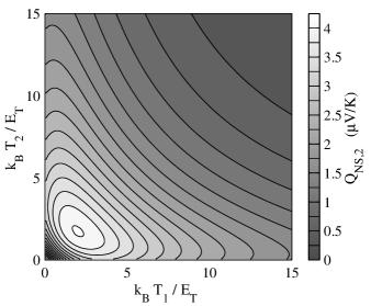
Figure 2: Temperature dependence of the N-S thermopower in a left–right-symmetric structure — $L_{j},\sigma_{j}$ and $A_{j}$ assumed equal. Phase $\phi=\pi/2$ is fixed.

The typical magnitude and form of the temperature dependence of ${Q_{\mathrm{NS}}}$ is shown in Fig. 2. The figure shows that the magnitude is ${Q_{\mathrm{NS}}}\sim\mathrm{\frac{\mu{}V}{K}}$ (often ${Q_{\mathrm{NS,1}}}\approx{Q_{\mathrm{NS,2}}}$), and that the relevant energy scale is $E_{T}$, corresponding to the link between the superconductors — which is also the energy scale of the spectral coefficients. Moreover, as shown in the preceding sections, the thermopower oscillates antisymmetrically with the phase difference (see Fig. 3).

The N-S thermopower shows re-entrant behavior: it vanishes as $T_{1},T_{2}\rightarrow 0$, peaks at an intermediate temperature, and decays as $T_{1},T_{2}\rightarrow\infty$. The peak near $T\sim 2E_{T}/k_{B}$ corresponds to the position where $I_{S}(T)$ changes rapidly as a function of the temperature, as Eqs. (25,26) indicate. Moreover, Eqs. (25,30) predict that ${Q_{\mathrm{NS}}}$ decays at least as $T^{-2}$ for $T_{1}\approx{}T_{2}$. In fact, Eq. (28) implies that the contribution from the supercurrent should decay exponentially, but the contribution from $\mathcal{T}$ has a slower speed of decay.

The most significant contribution to ${Q_{\mathrm{NS}}}$ is described by Eq. (25): it yields almost all of the effect seen in Fig. 2. The correction due to $\mathcal{T}$ accounts for the most of the deviation from the numerical result, and has an effect below 10% in relative magnitude for temperatures $T_{1},T_{2}\lesssim 10\leavevmode\nobreak\ E_{T}/k_{B}$, but the proportion becomes relatively larger at higher temperatures — see Fig. 5(a). Moreover, $\mathcal{D}_{T}$ has a negligible effect on ${Q_{\mathrm{NS}}}$, as seen in Fig. 5(a).

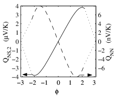
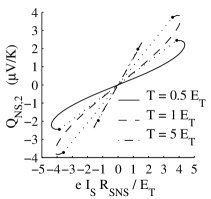
Figure 3: Oscillation of the thermopower. Left: Phase-oscillation of the thermopower at $T_{2}\approx{}T_{1}=1\leavevmode\nobreak\ E_{T}$. Right: Relation between ${Q_{\mathrm{NS}}}$ and the non-equilibrium supercurrent $I_{S}$ at different temperatures $T=T_{1}\approx{}T_{2}$. Magnitude of the supercurrent here is nearly the same as in equilibrium. Due to a numerical convergence problem, data for phases $|\phi|>2.1$ is not available, and hence substituted with straight line segments (dotted). In the right picture, the dotted part also approximately describes the accessible non-dissipative regime in the case when the supercurrent is externally driven.

The thermopower ${Q_{\mathrm{NS}}}$ with respect to the actual (non-equilibrium) supercurrent flowing in the structure is shown in Fig. 3. For a given temperature, the relation between ${Q_{\mathrm{NS}}}$ and $I_{S}$ appears to be linear, in accord with Eq. (25).

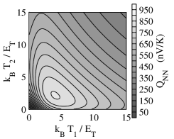
(a)

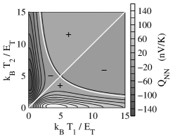
(b)

Figure 4: Temperature dependence of the N-N thermopower. Left: $Q_{\mathrm{NN}}$ in an asymmetric structure, $R_{3}/2=R_{1}=R_{2}=R_{4}=R_{5}$ with $A\sigma$ equal, at $\phi=\pi/2$. Right: $Q_{\mathrm{NN}}$ in a left–right-symmetric structure, where the $\mathcal{D}_{T}$-contribution dominates. The thick white lines indicate a change of sign for $R(T_{1})-R(T_{2})$, which occurs near the change of sign of $Q_{\mathrm{NN}}$.

The temperature dependence of $Q_{\mathrm{NN}}$ shown in Fig. 4(b) is very different from that of ${Q_{\mathrm{NS}}}$, since the structure there is assumed to be left–right symmetric, so that for $Q_{\mathrm{NN}}$ the contributions from $I_{S}$ and $\mathcal{T}$ vanish and the $\mathcal{D}_{T}$-effect dominates (see Fig. 5(b)). In this case, Eq. (32) predicts $\Delta\mu\propto(T_{1}-T_{2})^{2}$ at $T_{1}\approx{}T_{2}$ in symmetric structures, thus the thermopower appears only at large temperature differences, i.e. in the non-linear regime. For asymmetric structures, $\mathcal{D}_{T}$-effect is less important, as Eq. (31b) implies $\Delta\mu\propto(T_{1}-T_{2})$ at $T_{1}\approx{}T_{2}$, and this effect tends generally to wash out the $\mathcal{D}_{T}$-effect also at large temperature differences. This behavior can be seen in Fig. 4(a), where $Q_{\mathrm{NN}}$ has a similar temperature dependence as ${Q_{\mathrm{NS}}}$ in Fig. (2). Effects due to the sample geometry are discussed in more detail in the following section.

Note that the re-entrant temperature-dependent behavior of the conductance [14] induced by the proximity effect also arises due to the energy dependence of $\mathcal{D}_{T}$. Thus, the finite NN-thermopower in a left–right-symmetric structure may at least qualitatively be understood to be caused by an induced left–right asymmetry in the resistances, which makes the potential induced in the colder electrode different from the one in the hotter electrode. Indeed, the sign changes in Fig. 4(b) (along the diagonal and the $1/T_{1}$-like curve) occur close to the curves where the (zero-bias) conductances, [16]

$$G(T)=\int_{{0}}^{\infty}\!\tilde{R}^{-1}\;\frac{\operatorname{sech}^{2}(E/(2k_{B}{}T))}{2k_{B}T}\,\mathrm{d}E\,,\quad\tilde{R}\equiv\bigl{<}\mathcal{D}_{T}^{-1}\bigr{>}R\,,$$ (45)

of wires 1 and 2 at the temperatures $T_{1},T_{2}$ become equal. Approximately such behavior is also expected on the basis of Eq. (32).

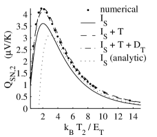
(a) ${{Q_{\mathrm{NS,2}}}}$ at $T_{1}\approx{}T_{2}$

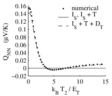
(b) $Q_{\mathrm{NN}}$ with fixed $T_{1}=3.6\leavevmode\nobreak\ E_{T}$

Figure 5: Thermopower at $\phi=\pi/2$ in a symmetric structure, $L$ and $A\sigma$ assumed equal for each wire. The numerical results and different analytic approximations from Sect. 3.6 are shown. Here, “$I_{S}$ (analytic)” is the approximation from Eq. 28.

Comparing to numerical results, we find that the approximations obtained from Eq. (24) in the long–junction limit are quantitatively accurate in a symmetric system, both for ${Q_{\mathrm{NS}}}$ and $Q_{\mathrm{NN}}$ (the relative error in ${Q_{\mathrm{NS}}}$ is less than 5% nearly everywhere in Fig. 2, although near $T_{1},T_{2}\approx 0$ it is $\sim 15\%$, at worst). In setups geometrically deformed from this, the accuracy may decrease slightly, but qualitative features are still well retained (in all cases tested). Equations  (24,25,30,32) may thus be used to provide useful approximations to the induced potentials, if the spectral coefficients are known.

5 DEPENDENCE ON SAMPLE GEOMETRY

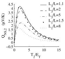
(a) ${{Q_{\mathrm{NS,2}}}}$

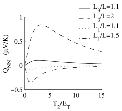
(b) $Q_{\mathrm{NN}}$

Figure 6: Thermopower in an asymmetric structure with all except one wire of length $L$, at $T_{1}\approx{}T_{2}$, $\phi=\pi/2$. $A\sigma$ assumed equal in all wires.

The thermopower induced by the proximity effect has a non-trivial dependence on the exact geometry of the structure: varying the geometry of the structure changes both the magnitudes and the temperature dependence of the induced potentials, as seen in Fig. 6. The changes arise partly in the kinetic equations, the effect of which is estimated by the prefactors in the approximations (25,30), but also the spectral equations contribute through the geometry dependence of the spectral coefficients — their behavior is discussed in Sect. 7

An effect visible in Fig. 6(a) is that compared to the symmetric structure, the induced potentials typically tend to be smaller in structures where the lengths of some of the wires are strongly different from each other. This behavior appears due to both the spectral coefficients and the kinetic equations. For example letting $L_{1,2}/L_{3,4,5}\rightarrow 0$ tends to decrease the thermopower, as then $I_{S}$ and $\bigl{<}\mathcal{T}_{\,}\bigr{>}$ are suppressed, while in the opposite limit most of the temperature drop occurs in wires 1 and 2 where there is little coupling between the charge and energy currents, leading again to a smaller thermopower (as indicated by the prefactors in Eqs. (25,30)).

The effect the geometry has on the induced potentials is more significant for $Q_{\mathrm{NN}}$ than for ${Q_{\mathrm{NS}}}$, since the contributions to $\Delta\mu$ depend strongly on the asymmetry and may also vanish due to symmetries in the structure. Generally, the approximations imply that in left–right-asymmetric structures, $Q_{\mathrm{NN}}$ should be finite and roughly resemble the N-S thermopower in temperature dependence, as in Fig. 4(a). Moreover, this thermopower should be discernible even for small amounts ($\sim 10\%$) of asymmetry in resistances, as can be seen in Fig. 6(b).

Although the temperature dependence of thermopower generally scales with $E_{T,SNS}$ similarly to the spectral coefficients, its exact form depends on the geometry of the structure. That is, the terms due to $j_{S}$ and $\bigl{<}\mathcal{T}_{\,}\bigr{>}$ appearing in the thermopower estimates vary in the geometry dependence, hence one can alter their relative weights by adjusting the structure. Moreover, they may also differ in sign and in the way they depend on the temperature, so their weighing has a direct effect on the temperature dependence of the thermopower. This is important especially for the N-N thermopower, which can be seen in Fig. 6(b) where changes in $L_{1}$ and $L_{3}$ cause qualitatively different results.

5.1 Thermopower and the central wire

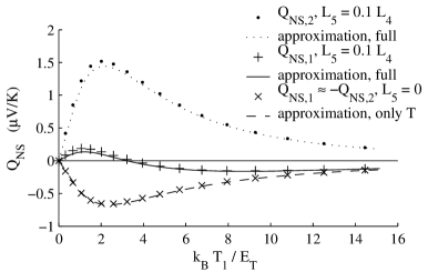
Figure 7: N-S thermopower for a structure with the central wire short or absent, $L_{1}=L_{2}=L_{4}$ and $A\sigma$ assumed equal. Moreover, $T_{1}\approx{}T_{2}$ and $\phi=\pi/2$. The “full analytic approximation” is obtained using Eq. (24) and numerical data for $\mathcal{D}_{T}$, $j_{S}$ and $\mathcal{T}$. The approximation for the contribution due to $\mathcal{T}$ obtained from Eq. (30) (dashed) is nearly the same in absolute value for all cases shown.

As found analytically in Sect. 3.6, the spectral coefficients that affect the thermopower most are $j_{S}$ and $\mathcal{T}$. In the long-junction limit, $j_{S}$ couples the energy and charge currents in the central wire, and $\bigl{<}\mathcal{T}_{1/2}\bigr{>}$ do this in the wires leading to the N-reservoirs. By changing the proportion of the lengths of these wires, using the factors in Eqs. (25,30) as a guide, the weaker effect due to $\bigl{<}\mathcal{T}_{\,}\bigr{>}$ may be brought to dominate. In the following, we consider a special case where $\mathcal{T}$ should manifest: $L_{5}\ll{}L_{SNS}$. (Another possibility suggested by Eqs. (25,30) would be $L_{1},L_{2}\gg{}L_{SNS}$, but in this case, the terms $\bigl{<}\mathcal{T}_{1/2}\bigr{>}$ become small.)

In the limit $L_{5}\,/\min[L_{1},L_{2},L_{3},L_{4}]\rightarrow 0$, the supercurrent-effect approximation (25) yields no contribution, and the second term in Eq. (30) vanishes, leaving only the contribution due to $\bigl{<}\mathcal{T}_{1/2}\bigr{>}$. If the structure is left–right-symmetric, then $\mathcal{T}_{1/2}=0$, and the thermopower also vanishes (confirmed by simulations). In fact, this can be shown exactly by noting that $f_{T}\equiv 0$ is the exact solution to the kinetic equations in this special case.

In asymmetric structures especially with $L_{3}\neq{}L_{4}$, generally $\bigl{<}\mathcal{T}_{1/2}\bigr{>}\neq 0$ and their sign is the same for both wires 1 and 2. Hence ${Q_{\mathrm{NS}}}$ becomes finite and there is a large difference between ${Q_{\mathrm{NS,1}}}$ and ${Q_{\mathrm{NS,2}}}$, as the contributions from Eq. (30) differ in sign for electrodes 1 and 2. In Fig. 7 the approximation (30) matches the numerical result well: $\bigl{<}\mathcal{T}_{1}\bigr{>}$ and $\bigl{<}\mathcal{T}_{2}\bigr{>}$ yield the dominant contribution.

As the terms (25) due to $I_{S}$ have the same sign for both electrodes and vanish as $L_{5}\rightarrow 0$, ${Q_{\mathrm{NS}}}$ may change its sign with increasing temperature for intermediate length $L_{5}$ of the central wire. This is possible because for a certain range of values for $L_{5}$, $I_{S}$ contributes the same overall amount as $\bigl{<}\mathcal{T}_{1/2}\bigr{>}$, but in the opposite direction for either ${Q_{\mathrm{NS,1}}}$ or ${Q_{\mathrm{NS,2}}}$. As the two contributions have slightly different temperature dependence, this can result in a change of sign in the thermopower, for a suitable $L_{5}$. The effect is illustrated in Fig. 7, where a change of sign occurs for $L_{5}=0.1L$. This sign change may partially explain the results in Ref. parsons03, see Subs. 6.1

5.2 Effect of decreasing $\Delta/E_{T}$

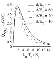
(a) ${Q_{\mathrm{NS}}}$, $T_{0}\approx{}T_{1}\approx{}T_{2}$

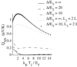
(b) $Q_{\mathrm{NN}}$, $T_{0}=T_{1}=3.6\leavevmode\nobreak\ E_{T}$

Figure 8: Thermopower for different $\Delta/E_{T}$. Left: ${Q_{\mathrm{NS}}}$ in a structure with all wires equal. Right: $Q_{\mathrm{NN}}$ in a structure with $L_{1}=L_{2}=L_{4}=L_{5}=L$ and $L_{3}=L$ or $L_{3}=2L$. In both figures, $A\sigma$ is assumed equal for all wires. The temperature dependence of $\Delta$ is neglected in the figures.

In reality, the superconducting energy gap $\Delta$ may be quite small in systems realized experimentally, and not necessarily much greater than $E_{T}$. For example, Eq. (12) shows that $\Delta=2$ K corresponds roughly to $10\leavevmode\nobreak\ E_{T}$ for $L_{SNS}=1\leavevmode\nobreak\ \mathrm{\mu{}m}$ and to $3\leavevmode\nobreak\ E_{T}$ for $L_{SNS}=0.5\leavevmode\nobreak\ \mathrm{\mu{}m}$, for a typical value $D=200\leavevmode\nobreak\ \mathrm{\frac{cm^{2}}{s}}$ of the diffusion constant.

For a finite $\Delta$, the spectral currents from the energies $E>\Delta$ contribute to the integrated currents. This in turn couples the temperature $T_{0}$ of the superconductors to the system, as seen in Eq. (24). Additionally, the spectral coefficients at energies $E<\Delta$ are modified from their long-junction limits, and hence the contribution from $E<\Delta$ is also affected.

Estimates for the effect due to the coupling of $T_{0}$ may be obtained from Eq. (24). Generally, terms proportional to $(f_{L,0}^{0}-f_{L,1}^{0})$, $(f_{L,0}^{0}-f_{L,2}^{0})$ and $(f_{L,1}^{0}-f_{L,2}^{0})$ appear for $E>\Delta$, thus any of the corresponding temperature differences induces potentials. However, these contributions tend to be smaller than those from $E<\Delta$, at least for $\Delta/E_{T}\gtrsim 10$ — supposing of course that $T_{1}-T_{2}$ is of the order $T_{1}-T_{0}$ or $T_{2}-T_{0}$, whichever is larger.

Figure 8(a) shows the effect of decreasing $\Delta/E_{T}$ on the N-S thermopower. The energy scale of the temperature dependence seems to be compressed towards $T=0$, but no significant qualitative changes occur. The result is similar if $T_{1}=T_{0}$ are kept fixed and $T_{2}$ is varied.

As $Q_{\mathrm{NN}}$ is generally smaller than ${Q_{\mathrm{NS}}}$, the relative changes tend to be larger in it. This can be seen in Fig. 8(b), where the contribution from $E>\Delta$ for $\Delta/E_{T}=10$ peaks near $T_{2}=6\leavevmode\nobreak\ E_{T}$ in the left–right-symmetric structure, and is also the dominant effect there. For the asymmetric structure, the change is relatively much less significant.

6 COMPARISON WITH RECENT WORK

In this section, we compare the theory presented in this paper and in Ref. virtanen04 to recent experiments and other theories on the thermopower in proximity effect structures.

6.1 Comparison to experiments

To our knowledge, there exist so far five published experiments from two groups probing the thermopower in Andreev interferometers [18, 19, 20, 21, 22]. One can distinguish three features of these experiments to which our theory can be compared: magnitude of the observed effect and the dependence on the temperature and magnetic flux.

In Ref. eom98, the temperature gradient produced by the heating current was not explicitly measured, but only estimated using a heating model. Such a procedure yielded too large an estimate (of the order of $\mu$V/K) for the measured NN-thermopower.[20] This observation is supported by Refs. dikin02,dikin02b, which discuss further measurements by the same group, now with the direct measurement of the temperature. Below, we concentrate on the results of Ref. dikin02 — the observations in Ref. dikin02b are quite analogous. These measurements yield a thermopower of the order of 50-60 nV/K at the temperature of the order of one Thouless temperature corresponding to the distance between the two superconductors. The measured structure slightly differed from that considered in our manuscript, as the superconductors were fabricated directly on top of the normal wires. However, we may assume the N-S contact resistances to play a similar role as the resistances of the wires 3 and 4 (see also Subs. 6.2). We also note that the magnitude of the NN thermopower greatly depends on the asymmetry in the structure. For example, taking the following estimates for the resistances of the five wires: $R_{1}=5\leavevmode\nobreak\ \Omega$, $R_{2}=5.5\leavevmode\nobreak\ \Omega$, $R_{3}=R_{4}=0.5\leavevmode\nobreak\ \Omega$, $R_{5}=5\leavevmode\nobreak\ \Omega$ (note that mostly only the ratios of the resistances are relevant) and assuming $E_{T}/k_{B}=275$ mK (corresponding to a wire of length 700 nm) we get $Q_{NN}=60$ nV/K at $T=295$ mK, $\phi=\pi/2$. This is very close to the experimental results.

Concerning a comparison to the experiments in Ref. parsons03, we obtain NS thermopower which is larger by an order of magnitude (of the order of 2 $\mu$V/K, whereas the experiments report some 70 nV/K). However, it is not totally clear to us where the normal-metal reservoirs in this experiment reside, and hence, which values should be used for the resistances $R_{1}$ and $R_{2}$.

Our theory predicts a nonmonotonic thermopower as a function of the lattice temperature, with a maximum at around $E_{T}/k_{B}$, given by the Thouless energy corresponding to the wire length between the superconductors. This is in agreement with Fig. 4 in Ref. eom98. The temperature scale of the dependence $Q(T)$ in Refs. parsons03,parsons03b is of the order of $E_{T}/k_{B}$, but these papers also report a sign reversal of the thermopower as a function of $T$. As indicated in Subs. 5.1, this may be possible in a suitable (left–right asymmetric) geometry where the overall supercurrent and $\mathcal{T}$-term contributions to the thermopower are comparable. Another possible source for the sign change is the additional term induced by the coupling of the superconductor temperature $T_{0}$ at high temperatures.

As shown in Subs. 3.4, the exact solution of our equations (within the assumption of electron-hole symmetry) is an antisymmetric function of the flux (phase) with respect to zero flux. This is in agreement with the symmetries obtained for the "Parallelogram" structure in Ref. eom98, and those measured in Refs. dikin02,dikin02b,parsons03,parsons03b. However, our results cannot explain the symmetric flux dependence seen in the "House" interferometer in Ref. eom98.

6.2 Comparison with other theories

The first theoretical discussion of thermoelectric phenomena under the superconducting proximity effect by Claughton and Lambert [17] showed how the thermoelectric coefficients can be calculated from the scattering theory. The general qualitative features one can extract from the analytic formulae are valid in any kind of structures composed of normal metals and superconductors. However, the numerical simulations of these systems (included, for example, in Refs. claughton96,heikkila00) suffer from the small size of the simulated structures which makes it difficult to differentiate between the effects related with electron-hole asymmetry (large in the small simulated structures) from the dominant effects in realistic experimental samples with thousands of channels.

In Refs. seviour00,kogan02, the thermopower of normal-superconducting structures is considered in the limit of a weak proximity effect (with large NS interface resistance) and in the linear regime. To compare our theory to those in their works, let us set $T_{2}=T_{0}+\delta T/2$, $T_{1}=T_{0}-\delta T/2$ in Eq. (25) for the S-N thermopower in a left–right symmetric structure,

$$Q_{SN}=\frac{\mu_{1,2}}{\delta T}=\frac{1}{4}\frac{R_{5}}{2R_{1,2}+R_{5}}\;\frac{1}{(k_{B}T_{0})^{2}}\;\int_{{0}}^{\infty}\!Ej_{S}^{\prime}\cosh^{-2}\left(\frac{E}{2k_{B}T_{0}}\right)\,\mathrm{d}E\,.$$ (46)

Here, $j_{S}^{\prime}=L_{3}j_{S}$. This is analogous to Eq. (7) in Ref. seviour00 and to the upper line of Eq. (8) in Ref. kogan02. The primary coefficient $g_{z+}$ in these equations is proportional to the spectral supercurrent across the normal-superconducting interface, analogous to $j_{S}^{\prime}$ in Eq. (46).

The lower line of Eq. (8) in Ref. kogan02 describes a thermopower arising between the normal-metal reservoirs. This term arises from the spectral supercurrent across the interface at the energies above the superconducting gap $\Delta$ and is thus similar to the contributions discussed in Subs. 5.2 As shown there, these contributions are mostly important only for highly left–right symmetric structures in the case when $L_{SNS}$ is not much larger than the superconducting coherence length, or when $T_{1}$ or $T_{2}$ are close to $\Delta/k_{B}$.

7 BEHAVIOR OF SPECTRAL COEFFICIENTS

Since the thermopower is induced by the spectral coefficients $j_{S}$ and $\bigl{<}\mathcal{T}\bigr{>}$, we describe here briefly their dependence on the energy and on the sample geometry.

7.1 Spectral supercurrent

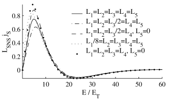
Figure 9: The spectral supercurrent $j_{S}$ for different ratios of wire lengths.

The spectral supercurrent $j_{S}$ is the better-known of the two main contributors for the thermopower. In structures such as considered here, it typically has the energy dependence shown in Fig. 9: the characteristic energy scale is $E_{T,SNS}$, and the dimensionless quantity $L_{SNS}j_{S}$ does not depend greatly on the exact geometry of the structure (supposing $L_{1},L_{2}\gtrsim{}L_{SNS}$). The behavior of $j_{S}$ is discussed in detail in Ref. heikkila02scdos, and the results are also mostly applicable to the structure considered here, as the central wire typically causes no significant qualitative changes.

7.2 Anomalous $\mathcal{T}$-term

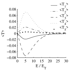
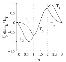
Figure 10: Behavior of $\mathcal{T}$ in a structure with $L_{1}=L_{2}=L_{3}/1.1=L_{4}=L_{5}$ and $A\sigma$ equal, at $\phi=\pi/2$. Left: The energy-dependence of the averaged dimensionless coefficient $\bigl{<}\mathcal{T}_{\,}\bigr{>}=\frac{1}{L_{k}}\int_{{0}}^{L_{k}}\!\mathcal{T}\,\mathrm{d}x$ in different wires. Right: Spatial behavior of $\int_{{0}}^{\infty}\!\mathcal{T}\,\mathrm{d}E/E_{T}$. Different branches correspond to $\mathcal{T}_{k}$ in different wires. Locations of the two nodes are indicated by the dotted lines, and reservoir interfaces are denoted by dots.

The $\mathcal{T}$-term (8d), whose effect is neglected in most previous papers, is a coefficient appearing in the non-equilibrium part of the supercurrent, and it has no clear physical interpretation. Nonetheless, it affects the potentials induced due to a temperature difference, and provides in some cases the dominant contribution which may be large by itself. Hence it is interesting to examine the energy and spatial behavior of this coefficient, which is here considered in the long-junction limit $\Delta\gg E_{T}$.

The typical energy dependence of the average $\mathcal{T}$ in different wires of the structure in Fig. 1 is shown in Fig. 10. Its magnitude is approximately less than 10% of the spectral supercurrent $L_{SNS}j_{S}$, but the energy dependence is rather similar: a single peak appears on the scale of $E_{T,SNS}$ although there is less oscillation than in $L_{SNS}j_{S}$.

The spatial dependence shown in Fig. 10 gives insight to the magnitudes of $\mathcal{T}$ in different wires. Here, $\mathcal{T}$ vanishes at the reservoirs and changes its sign near the center of the SNS link, forming peaks between the S-reservoirs and the center. This leads to $\bigl{<}\mathcal{T}_{5}\bigr{>}\approx 0$ in nearly left–right-symmetric structures, as seen in Fig. 10. Moreover, $\mathcal{T}_{3}$ and $\mathcal{T}_{4}$ are typically the largest and the two differ in sign.

In the wires 1 and 2 leading to the N-reservoirs, $\mathcal{T}$ decays monotonically to zero on the length scale of $L_{SNS}$ (according to numerical results). In fact, no sign changes are possible for $\mathcal{T}_{1/2}$, as $\chi\equiv\textrm{const}(x)$ in these wires. Moreover, note that for the quantities $\bigl{<}\mathcal{T}_{1/2}\bigr{>}$ relevant for the thermopower, this kind of a decay would imply that $\bigl{<}\mathcal{T}_{1/2}\bigr{>}$ vanish for $L_{1,2}/L_{SNS}\rightarrow\infty$.

The magnitude and the sign of $\mathcal{T}$ in the wires 1 and 2 depend on the points where the wires are connected to the SNS link, since $\mathcal{T}$ is continuous in the structure. Moreover, if the N-reservoirs are far ($L_{1},L_{2}\gtrsim{}L_{SNS}$), the choice of the connection points does not affect much the $\mathcal{T}$ in the SNS link, hence one may estimate the qualitative behavior of $\mathcal{T}$ in wires 1 and 2 by looking at Fig. 10.

Using the symmetry arguments from Subs. 3.4, one finds that $\mathcal{T}$ oscillates antisymmetrically with the phase difference. Moreover, the overall phase behavior of $\mathcal{T}$ seems to be similar to that of $j_{S}$, according to numerical results.

8 DISCUSSION

In this paper, we have shown how the presence of the supercurrent can lead to a finite thermopower in an Andreev interferometer even in the presence of complete electron-hole symmetry. Generally, the thermopower probes the temperature dependence of the supercurrent, which in the long-junction limit is determined by the Thouless energy corresponding to the distance between the superconductors. The actual magnitude of the thermopower also strongly depends on the studied geometry of the sample, which has to be taken into account when comparing to the experiments.

Another interesting result is the thermopower induced by the "anomalous" coefficient $\mathcal{T}$. This coefficient has been identified in a number of theoretical publications (for example, Refs. seviour00,kogan02,heikkila03,yip98,lee99,bezuglyi03b — it is frequently referred to as the "anomalous current" as its properties are not very well known) but typically its effect is neglected and we are not aware of any other observable whose behavior would be dictated by $\mathcal{T}$.

The theory presented in this paper and in Ref. virtanen04 seems to be in fair agreement with most of the experimental results published so far (see Subs. 6.1). However, unless device geometry (resistances of the wires) are quite well known, it is difficult to make a detailed comparison of the magnitude and temperature dependence of the measured thermopower. There exists also one experimental result (the symmetric oscillations of the thermopower in the "House" interferometer in Ref. eom98) which clearly cannot be explained with the present theory.

Confirming the theory clearly calls for more experiments on the subject. Rather than as a function of the applied flux, one could probe the thermopower by externally applying a supercurrent between the superconductors (c.f., Fig. 3). In this way, one would also be able to compare the observed thermopower to the temperature dependence of the equilibrium (critical) supercurrent, essentially with no fitting parameters — the normal-state resistances can be fairly accurately measured in the considered multiprobe structure. Further, it would be interesting to confirm the relation between the thermopower and the "anomalous" term $\mathcal{T}$, either by substracting the supercurrent part from the results or, for example, in a structure without the central wire. The effect of the additional terms, present in short wires (due to a finite $\Delta/E_{T}$) or highly symmetric structures (due to the proximity-induced temperature dependence in the resistances), would also be worth studying, but perhaps more difficult to realize in practice.

References

-
[1]
V. L. Ginzburg.
Nobel lecture (2003).
http://www.nobel.se/physics/laureates/2003/ginzburg-lecture.html. - [2] V. L. Ginzburg. Zh. Éksp. Teor. Fiz., 14, 177 (1944). [J. Phys. USSR 8, 148 (1944)].
- [3] N. W. Ashcroft and N. D. Mermin. Solid-state physics. Saunders College Publishing (1967). Chapters 12–13.
- [4] D. J. van Harlingen. Physica, 109 & 110B, 1710 (1982).
- [5] Y. M. Galperin, V. L. Gurevich, V. I. Kozub, and A. L. Shelankov. Phys. Rev. B, 65, 064531 (2002).
- [6] C. J. Pethick and H. Smith. Phys. Rev. Lett., 43, 640 (1979).
- [7] J. Clarke, B. R. Fjordbøge, and P. E. Lindelof. Phys. Rev. Lett., 43, 642 (1979).
- [8] A. Schmid and G. Schön. Phys. Rev. Lett., 43, 793 (1979).
- [9] J. Clarke and M. Tinkham. Phys. Rev. Lett., 44, 106 (1980).
- [10] C. J. Lambert and R. Raimondi. J. Phys.: Condens. Matter, 10, 901 (1998).
- [11] H. Courtois and B. Pannetier. J. Low Temp. Phys., 118, 599 (2000).
- [12] W. Belzig, F. K. Wilhelm, C. Bruder, G. Schön, and A. D. Zaikin. Superlatt. Microstruct., 25, 1251 (1999).
- [13] P. Dubos, H. Courtois, B. Pannetier, F. K. Wilhelm, A. D. Zaikin, and G. Schön. Phys. Rev. B, 63, 064502 (2001).
- [14] P. Charlat, H. Courtois, Ph. Gandit, D. Mailly, A. F. Volkov, and B. Pannetier. Phys. Rev. Lett., 77, 4950 (1996).
- [15] Yu. V. Nazarov and T. H. Stoof. Phys. Rev. Lett., 76, 823 (1996).
- [16] E. V. Bezuglyi and V. Vinokur. Phys. Rev. Lett., 91, 137002 (2003).
- [17] N. R. Claughton and C. J. Lambert. Phys. Rev. B, 53, 6605 (1996).
- [18] J. Eom, C.-J. Chien, and V. Chandrasekhar. Phys. Rev. Lett., 81, 437 (1998).
- [19] D. A. Dikin, S. Jung, and V. Chandrasekhar. Phys. Rev. B, 65, 012511 (2002).
- [20] D. A. Dikin, S. Jung, and V. Chandrasekhar. Europhys. Lett., 57, 564 (2002).
- [21] A. Parsons, I. A. Sosnin, and V. T. Petrashov. Phys. Rev. B, 67, 140502 (2003).
- [22] A. Parsons, I. A. Sosnin, and V. T. Petrashov. Physica E, 18, 316 (2003).
- [23] T. T. Heikkilä, M. P. Stenberg, M. M. Salomaa, and C. J. Lambert. Physica B, 284-8, 1862 (2000).
- [24] R. Seviour and A. F. Volkov. Phys. Rev. B, 62, 6116 (2000).
- [25] V. R. Kogan, V. V. Pavlovskii, and A. F. Volkov. Europhys. Lett., 59, 875–881 (2002).
- [26] P. Virtanen and T. T. Heikkilä. Phys. Rev. Lett. 92, 177004 (2004).
- [27] T. T. Heikkilä, T. Vänskä, and F. K. Wilhelm. Phys. Rev. B, 67, 100502(R) (2003).
- [28] Y. V. Nazarov. Superlatt. Microstruct., 25, 1221 (1999).
- [29] J. Rammer and H. Smith. Rev. Mod. Phys., 58, 323 (1986).
- [30] K. D. Usadel. Phys. Rev. Lett., 25, 507 (1970).
- [31] T. T. Heikkilä, J. Särkkä, and F. K. Wilhelm. Phys. Rev. B, 66, 184513 (2002).
- [32] W. Hänsch. Phys. Rev. B, 31, 3504 (1984).
- [33] F. K. Wilhelm, G. Schön, and A. D. Zaikin. Phys. Rev. Lett., 81, 1682 (1998).
- [34] S.-K. Yip. Phys. Rev. B, 58, 5803 (1998).
- [35] S.-W. Lee, A. V. Galaktionov, and C.-M. Ryu. J. Korean Phys. Soc., 34, S193 (1999).
- [36] E. V. Bezuglyi, V. S. Shumeiko, and G. Wendin. Phys. Rev. B, 68, 134506 (2003).