Slip behavior in liquid films on surfaces of patterned wettability:
Comparison between continuum and molecular dynamics simulations

Abstract

We investigate the behavior of the slip length in Newtonian liquids subject to planar shear bounded by substrates with mixed boundary conditions. The upper wall, consisting of a homogenous surface of finite or vanishing slip, moves at a constant speed parallel to a lower stationary wall, whose surface is patterned with an array of stripes representing alternating regions of no-shear and finite or no-slip. Velocity fields and effective slip lengths are computed both from molecular dynamics (MD) simulations and solution of the Stokes equation for flow configurations either parallel or perpendicular to the stripes. Excellent agreement between the hydrodynamic and MD results is obtained when the normalized width of the slip regions, $a/\sigma\gtrsim{\cal O}(10)$, where $\sigma$ is the (fluid) molecular diameter characterizing the Lennard-Jones interaction. In this regime, the effective slip length increases monotonically with $a/\sigma$ to a saturation value. For $a/\sigma\lesssim{\cal O}(10)$ and transverse flow configurations, the non-uniform interaction potential at the lower wall constitutes a rough surface whose molecular scale corrugations strongly reduce the effective slip length below the hydrodynamic results. The translational symmetry for longitudinal flow eliminates the influence of molecular scale roughness; however, the reduced molecular ordering above the wetting regions of finite slip for small values of $a/\sigma$ increases the value of the effective slip length far above the hydrodynamic predictions. The strong correlation between the effective slip length and the liquid structure factor representative of the first fluid layer near the patterned wall illustrates the influence of molecular ordering effects on slip in non-inertial flows.

I Introduction

The development of micro- and nanofluidic devices for the manipulation of films, drops and bubbles requires detailed knowledge of interfacial phenomena and small scale flows. These systems, which are distinguished by a large surface-to-volume ratio and flow at small Reynolds, capillary and Bond numbers, are strongly influenced by boundary effects Darhuber05 . Liquid affinity to nearby solid boundaries can be reduced through chemical treatments Schnell56 ; Baudry01 ; Meinhart02 ; Breuer03 , substrate topology Watanabe99 ; Bocquet03 ; Krupenkin or the nucleation of nanobubbles on hydrophobic glass surfaces Ishida00 ; Tyrrell01 ; Steitz03 . Weak van der Waals interactions between a polymer melt and solid wall Leger97 ; Denn01 ; Leger03 or between two immiscible polymers Wyart90 can also lead to significant slippage and reduced frictional resistance. The degree of slip is normally quantified through the slip length defined as the distance from the surface within the solid phase where the extrapolated flow velocity vanishes Navier . Numerous experimental and theoretical studies have examined how the slip length is influenced by such factors as the degree of hydrophobicity Schnell56 ; Vinogradova99 , the substrate topography and surface roughness Watanabe99 ; Bocquet03 ; Richardson73 ; Hocking76 ; Jansons88 ; Einzel90 ; Davis94 ; Barrat94 ; Cottin , the presence of interstitial lubricating layers Davis94 ; Barnes95 ; Vinogradova03 , the polymer molecular weight Migler93 ; Archer ; Denn01 and the applied shear rate Nature97 ; Priezjev04 ; Vinogradova00 ; Granick01 ; Breuer03 . In a recent development, the large values of the slip length extracted from experiments involving the pressure-driven flow of water through hydrophobically coated capillaries have been attributed Vinogradova95 ; Stone03 to the spontaneous nucleation of a dense and stable layer of nanobubbles in water films adjacent to hydrophobic glass surfaces Ishida00 ; Tyrrell01 ; Steitz03 . Of special interest is the corresponding reduction in drag achieved by proportional substitution of liquid-solid contact area with liquid-gas contact area or equivalently, substitution of regions of no-slip or finite slip by regions of essentially no-shear (i.e. infinite slip).

Interest in the hydrodynamic behavior of liquid films in the vicinity of surfaces with mixed boundary conditions dates back several decades to the work of Philip Philip1 ; Philip2 . He examined the steady flow of an incompressible and inertia-less Newtonian liquid driven either by a uniform shear stress or uniform pressure gradient and subject to mixed wall boundary conditions. These were represented by surfaces consisting of alternating striped regions of no-shear and no-slip among other geometries. Using conformal mapping, Philip Philip1 ; Philip2 derived analytic expressions for the streamfunction and volumetric flux for flow perpendicular (transverse configuration) or parallel (longitudinal configuration) to the striped array in the limit of Stokes flow. Recently, Lauga and Stone Stone03 investigated the behavior of the effective slip length for steady Poiseuille flow through a capillary of circular cross-section whose inner wall consists of periodically distributed regions of no-slip and no-shear. Philip’s earlier treatment was used to extract the slip length for longitudinal configurations; additional analysis was required for transverse configurations. Comparison of their results with available experimental measurements suggests what model parameter values would reproduce the experimental slip lengths. For slip lengths in the nanometer range, one might ask whether a hydrodynamic analysis can correctly predict these values or whether the molecular aspects of the fluid can strong influence the slip behavior causing deviations from the continuum theory.

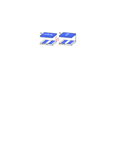
Figure 1: (Color online) (a) Transverse and (b) longitudinal flow orientations for a liquid film subject to planar shear in a cell with wall separation $d$. Darker stripes of width $a$ signify regions of finite slip or no-slip. White stripes signify regions of no-shear (or equivalently perfect slip). The upper wall moves at constant speed $U$ relative to the lower stationary surface ($z\!=\!0$). The periodicity of the lower wall pattern geometry is designed by $\lambda$.

Molecular dynamics (MD) simulations provide an ideal tool for investigating the conformation and behavior of fluid molecules adjacent to chemically or topologically textured substrates. The boundary conditions which establish the flow profile are not specified a priori, but arise naturally from the wall-fluid contrast in density and the fluid-fluid and wall-fluid interaction potentials. In recent years, many groups have examined how various molecular parameters characterizing the wall and fluid properties affect the degree of slip at liquid-solid interfaces. In particular, it has been demonstrated that the structure factor and contact density representative of the first fluid layer adjacent to a wall significantly influence the degree of slip in Newtonian and non-Newtonian fluids Thompson90 ; Thompson92 ; Thompson95 ; Barrat94 ; Nature97 ; Barrat99 ; Priezjev04 . The results of this current study confirm the importance of these molecular parameters for flow on heterogeneous substrates.

In this work, we investigate the behavior of the slip length in viscous films under planar shear bounded by substrates with mixed boundary conditions using both molecular dynamics (MD) simulations and Stokes flow computations. The upper wall, consisting of a homogenous surface of finite or no-slip, moves at a constant speed, $U$, a distance $d$ above a lower stationary wall, whose surface is patterned with an infinite array of stripes representing alternating regions of no-shear and finite or no-slip. As shown in Fig. 1, we consider transverse and longitudinal flow configurations and compute the corresponding velocity fields and effective slip lengths for a wide range of stripe widths, periods and liquid-solid affinities. Excellent agreement between the hydrodynamic and MD results is obtained when the normalized width of the slip regions, $a/\sigma\gtrsim{\cal O}(10)$, where $\sigma$ is the (fluid) molecular diameter characterizing the Lennard–Jones interaction. For surface patterns approaching molecular size, the degree of fluid ordering near the patterned wall, as quantified by the in-plane structure factor and contact density in the first liquid layer, plays a dominant role causing significant deviations from the hydrodynamic predictions. These deviations can be explained in the context of effective surface roughness and molecular ordering effects.

II Hydrodynamic Analysis

In the limit of vanishingly small Reynolds number ${\sf Re}\!=\!\rho Ud/\mu$, where $\rho$ and $\mu$ denote the (constant) liquid density and viscosity, inertial effects are negligible. The velocity profile is then governed by the Stokes equation, $\nabla^{2}{\bf u}\!=\!\nabla p/\mu$, where the velocity field, ${\bf u}$, satisfies the condition of incompressibility, $\nabla\!\cdot\!{\bf u}\!=\!0$, and $p$ denotes the pressure distribution which in this study is induced by the patterned substrates. Application of the divergence operator to the Stokes equation shows that the pressure field satisfies the equation $\nabla^{2}p\!=\!0$. It then follows that the velocity field satisfies the biharmonic equation $\nabla^{2}\nabla^{2}{\bf u}=0$ Leal92 .

In the next section, we derive the boundary conditions (BCs) corresponding to transverse [Fig. 1(a)] and longitudinal [Fig. 1(b)] flow orientations. These conditions are used to compute numerical solutions of the streamfunction, velocity field and effective slip length as a function of the dimensionless stripe width of the finite slip regions, $a/\lambda$, and the dimensionless surface period $\lambda/d$. The $\hat{y}$-axis is oriented parallel to the stripe edges for either configuration. All numerical calculations were performed with the finite element software FemLab 2.3 Femlab ; Wass04 using triangular elements with quadratic basis functions. The solutions reported converged upon mesh refinement.

II.1 Transverse configuration

The two dimensional velocity field corresponding to the transverse configuration shown in Fig. 1(a) is represented by ${\bf u}(x,z)\!=\!(u,0,w)=\!(\partial\psi/\partial z,0,-\partial\psi/\partial x)$, where $\psi(x,z)$ denotes the streamfunction, which implicitly satisfies the continuity equation $\nabla\!\cdot\!{\bf u}\!=\!0$. The vorticity vector ${\bf\Omega}\!=\!\nabla\!\times{\bf u}\!=\!(0,\omega,0)$, where $\omega=\partial u/\partial z\!-\!\partial w/\partial x$, has only one non-zero component. According to these definitions, it follows that

$$\omega=\frac{\partial^{2}\psi}{\partial z^{2}}+\frac{\partial^{2}\psi}{\partial x^{2}}={\nabla}^{2}\psi\ \ \ \ \ \mbox{and}\ \ \ \ \ {\nabla}^{2}\omega=0.$$ (1)

II.1.1 Boundary Conditions

Solutions of the equations for the vorticity and streamfunction given by Eq. (1) require the specification of eight BCs. The computational domain sketched in Fig. 2(a) is defined by the region bounded by the upper and lower walls ($0\!\leq\!z\!\leq\!d$) and the dashed lines ($0\!\leq\!x\!\leq\!\lambda/2$) corresponding to the midplanes of neighboring stripes. White surfaces designate shear-free boundaries (i.e. surfaces of perfect slip); dark surfaces designate boundaries of finite or no-slip. Throughout, partial derivatives are denoted by letter subscripts e.g. $\partial\psi/\partial x\equiv\psi_{x}$.

The top and bottom walls represent impenetrable surfaces where $w(x,z\!=\!0)=w(x,z\!=\!d)\!=\!0$, or in terms of the streamfunction, $\psi_{x}(x,z\!=\!0)\!=\!\psi_{x}(x,z\!=\!d)\!=\!0$. The tangential component of the velocity field must satisfy mixed slip and shear conditions at the upper and lower walls of the cell. The no-shear BC is given by $u_{z}(0\!\leq\!x\!\leq\!\frac{\lambda-a}{2},z\!=\!0)=0$. Slip surfaces are characterized by the Navier Navier slip condition $u\left[\frac{\lambda-a}{2}\!\leq\!x\!\leq\!\frac{\lambda}{2},z\!=\!0\right]=bu_{z}$ and $u[x,z\!=\!d]\!=\!U\!-\!bu_{z}$. The Navier slip length $b$ is assumed constant, i.e. independent of the shear rate $\dot{\gamma}$.

The lateral boundary conditions for the scalar field $u$ are derived from the following symmetry considerations. The biharmonic equation $\nabla^{2}\nabla^{2}u\!=\!0$ involves $x$-derivatives of even order only. The lower wall comprises an infinite number of mirror symmetry planes located at the at the stripe centers $x\!=\!n\lambda/2$, for all integers $n$. Since the upper surface is homogeneous and translationally invariant, the mirror symmetry imposed by the lower surface determines which symmetry applies throughout the entire Couette cell. The scalar field, $u$, therefore also assumes mirror symmetry about the stripe centers such that $u(x,z)\!=\!u(-x,z)$ and $u_{x}(x,z)\!=\!0$ for all $x\!=\!n\lambda/2$ and integers $n$. From the continuity equation, it then also follows that $w_{z}(x\!=\!n\lambda/2)=0$, i.e. $w$ is independent of the coordinate $z$ within any mirror plane. Since the upper and lowers walls are impenetrable, i.e. $w(x,z\!=\!0)=w(x,z\!=\!d)\!=\!0$, this constraint reduces to the BC $\psi_{x}(x\!=\!0)=0=\psi_{x}(x\!=\!\lambda/2)$.

The continuity equation requires $u_{x}+w_{z}=0$. Together with the condition $u(x,z)=u(-x,z)$, this implies $w(x,z)=-w(-x,z)$ such that $w(x,z)\!=\!0$ and $w_{xx}(x,z)=0$ at all $x=n\lambda/2$ where $n=0,1,2\ldots$. Substitution of this last relation and $u_{x}(x\!=\!0,z)=0$ into the expression for $\omega_{x}$ leads to $\omega_{x}(x\!=\!n\lambda/2,z)=0$. Regions of no-shear at the lower wall are represented by the condition $\omega(x,z\!=\!0)=0$.

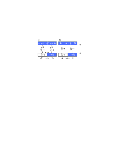
Figure 2: (Color online) Computational domain and boundary conditions used for solution of the Stokes equation corresponding to the (a) transverse and (b) longitudinal flow orientation shown in Fig. 1. The computational domain consists of the region bounded by the upper and lower walls ($z\!=\!0$ and $z\!=\!d$) and the lateral dashed lines ($x\!=\!0$ and $x\!=\!\lambda/2$), which are positioned at neighboring midplanes of the no-shear and finite-slip regions.

Along the top and bottom walls, the scalar component $w$ is independent of the coordinate $x$ and therefore $w_{x}(z\!=\!0)=w_{x}(z\!=\!d)=0$. Consequently, the vorticity at the top and bottom walls reduces to $\omega=u_{z}$ and the Navier slip conditions can be rewritten as $\psi_{z}\left(\frac{\lambda-a}{2}\!\leq\!x\!\leq\!\frac{\lambda}{2},z\!=\!0\right)=b\omega$ and $\psi_{z}(x,z\!=\!d)=U-b\omega$. The relation $w(x,z\!=\!0)=w(x,z\!=\!d)=\psi_{x}=0$ also implies that the streamfunction is constant in the planes $z\!=\!0$ and $z\!=\!d$, whose values we denote by $\psi_{\rm top}$ and $\psi_{\rm bottom}$. The difference in the streamfunction value between the top and bottom walls is equal to the volumetric flux per unit length along the $y$-axis Leal92 since

$$Q=\int\limits_{z=0}^{z=d}\!u(x,z)\,dz=\int\limits_{z=0}^{z=d}\!\psi_{z}\,dz=\psi_{\rm top}-\psi_{\rm bottom}~{}.$$ (2)

Because the streamfunction can only be determined within an arbitrary constant, we set the value of $\psi_{\rm bottom}$ in these studies to zero without loss in generality. The complete set of BCs for the vorticity and streamfunctions are therefore given by:

$$\psi(x,z\!=\!0) = 0$$ (3)

$$\psi(x,z\!=\!d) = \psi_{\rm top}$$ (4)

$$\omega(x,z\!=\!0) = 0\ \ \ \ \ \ \mbox{for $0\leq x<\frac{\lambda-a}{2}$}$$ (5)

$$\psi_{z}(x,z\!=\!0) = b\omega\ \ \ \ \mbox{for $\frac{\lambda-a}{2}\leq x\leq\frac{\lambda}{2}$}$$ (6)

$$\psi_{z}(x,z=d) = U-b\omega$$ (7)

$$\psi_{x}(x\!=\!0,z) = 0\ =\ \psi_{x}(x\!=\!\lambda/2,z)$$ (8)

$$\omega_{x}(x\!=\!0,z) = 0\ =\ \omega_{x}(x\!=\!\lambda/2,z)~{}.$$ (9)

II.1.2 Solution procedure

The value of $\psi_{\rm top}$ is determined from the pressure field as follows. The Stokes equation for the vertical component of the velocity field is given by $w_{xx}+w_{zz}\!=\!p_{z}/\mu$. As argued in a previous section, however, $w_{xx}(x\!=\!n\lambda/2,z)\!=\!0$, and since $w$ is independent of $z$ along any mirror symmetry plane, $w_{zz}(x\!=\!n\lambda/2,z)\!=\!0$. The pressure is therefore independent of the vertical coordinate $z$ in all planes $x\!=\!n\lambda/2$. Furthermore, in the absence of any externally applied pressure gradient, as is the case here, and because of the flow periodicity, $p(x\!=\!0)=p(x\!=\!\lambda)$. Since it was previously argued that $u$ exhibits mirror symmetry about the planes $x\!=\!n\lambda/2$, it must also be true of $p_{x}$ since $u_{xx}+u_{zz}\!=\!p_{x}/\mu$. Consequently, the pressure is equal at the lateral boundaries of the computational cell, i.e. $p(x\!=\!0)=p(x\!=\!\lambda/2)$. For convenience we set $p(x\!=\!0)\!=\!0$. This constraint, coupled with the relation $p_{x}/\mu\!=\!-(\nabla\times{\bf\Omega})\cdot\hat{e}_{x}=\omega_{z}$, was used to adjust the numerical value of $\psi_{\rm top}$ by requiring that the following integral vanish identically:

$$\int_{0}^{\lambda/2}\!\!p_{x}\,dx=\mu\int_{0}^{\lambda/2}\!\omega_{z}\,dx\ =0~{}.$$ (10)

The value of the effective slip length, $L_{s}$, corresponding to the overall flow within a patterned cell was obtained from linear extrapolation of the averaged velocity profile $\langle u\rangle\!=\!(2/\lambda)\int_{0}^{\lambda/2}u(x,z)\,dx$ to zero. Since at planes of mirror symmetry, $u_{x}\!=\!0$ and $p(x\!=\!0)=p(x\!=\!\lambda/2)$, the integral $\mu\int_{0}^{\lambda/2}\nabla^{2}u(x,z)dx=\int_{0}^{\lambda/2}p_{x}dx\!=\!0$, reduces to $\langle u\rangle_{zz}\!=\!0$. The averaged velocity field, $\langle u\rangle$, is therefore a linear function of $z$ and geometric similarity establishes the relation for the effective slip length, namely

$$\frac{L_{s}}{d}=\frac{\langle u(z\!=\!0)\rangle}{\langle u(z\!=\!d)\rangle-\langle u(z\!=\!0)\rangle}~{}~{}.$$ (11)

For the numerical analysis, the equations for the vorticity and streamfunction given by Eq. (1) and the BCs given by Eqs. (3-9) were non-dimensionalized according to the rescaled variables

$$\widetilde{x} = x/\lambda\ \ \ \ \ \ \ \ \ \ \ \ \ \ \widetilde{z}=z/d$$ (12)

$$\widetilde{u} = u/U\ \ \ \ \ \ \ \ \ \ \ \ \ \widetilde{w}=w\left/\left(U\frac{d}{\lambda}\right)\right.$$ (13)

$$\widetilde{\psi} = \psi\left/\left(\frac{Ud}{2}\right)\right.\ \ \ \widetilde{\omega}=\omega\left/\left(\frac{U}{d}\right)\right.~{},$$ (14)

leading to

$$\frac{d^{2}}{\lambda^{2}}\frac{\partial^{2}\widetilde{\psi}}{\partial\widetilde{x}^{2}}+\frac{\partial^{2}\widetilde{\psi}}{\partial\widetilde{z}^{2}}=2\widetilde{\omega}\ \ \ \ \ \mbox{and}\ \ \ \ \ \frac{d^{2}}{\lambda^{2}}\frac{\partial^{2}\widetilde{\omega}}{\partial\widetilde{x}^{2}}+\frac{\partial^{2}\widetilde{\omega}}{\partial\widetilde{z}^{2}}=0~{}.$$ (15)

In Section II.1.4 we present numerical solutions to Eqs. (15) and the extracted values of $L_{s}$ as a function of the local slip length $b$ and pattern geometry. Analytic expressions are derived in the limits $\lambda/d\rightarrow 0$ and $\lambda/d\rightarrow\infty$.

II.1.3 Perturbative analysis for $b=0$

In order to enhance the numerical precision of solutions corresponding to small values of $L_{s}$, the velocity and pressure fields were decomposed into two contributions, ${\bf u}\!=\!{\bf u}_{0}+{\bf u}_{1}$ and $p\!=\!p_{0}+p_{1}$. Here, ${\bf u}_{0}\!=\!(Uz/d,0,0)$ and $p_{0}\!=\!0$ correspond to the velocity and pressure fields for planar shear flow subject to no-slip at both solid boundaries. The Stokes equation then reduces to the form $\mu\nabla^{2}{\bf u}_{1}\!=\!\nabla p_{1}$, where the perturbed velocity field satisfies the continuity equation $\nabla\!\cdot\!{\bf u}_{1}\!=\!0$. The following BCs for the perturbed streamfunction and vorticity fields were determined in similar fashion as those in Section II.1.1:

$$\psi_{1}(x,z\!=\!0) = 0$$ (16)

$$\psi_{1}(x,z\!=\!d) = \psi_{1,{\rm top}}$$ (17)

$$\psi_{1,z}(x,z=d) = U$$ (18)

$$\omega_{1}\left(\mbox{$0\!\leq\!x\!<\!\frac{\lambda-a}{2}$},z\!=\!0\right) = -U/d$$ (19)

$$\psi_{1,z}\left(\mbox{$\frac{\lambda-a}{2}\!\leq\!x\!\leq\!\frac{\lambda}{2}$},z\!=\!0\right) = 0$$ (20)

$$\psi_{1,x}(x\!=\!0,z) = 0\ =\ \psi_{1,x}\left(\mbox{$x\!=\!\frac{\lambda}{2}$},z\right)$$ (21)

$$\omega_{1,x}(x\!=\!0,z) = 0\ =\ \omega_{1,x}\left(\mbox{$x\!=\!\frac{\lambda}{2}$},z\right)$$ (22)

where $\psi_{1,z}\!=\!u_{1}$, $\psi_{1,x}\!=\!-w_{1}$ and $\omega_{1}\!=\!u_{1,z}-w_{1,x}$. Non-dimensionalization of the vorticity and streamfunction perturbations $\omega_{1}$ and $\psi_{1}$ as in Section II.1.2 leads to:

$$\frac{d^{2}}{\lambda^{2}}\frac{\partial^{2}\widetilde{\psi}_{1}}{\partial\widetilde{x}^{2}}+\frac{\partial^{2}\widetilde{\psi}_{1}}{\partial\widetilde{z}^{2}} = 2\widetilde{\omega}_{1}$$ (23)

$$\frac{d^{2}}{\lambda^{2}}\frac{\partial^{2}\widetilde{\omega}_{1}}{\partial\widetilde{x}^{2}}+\frac{\partial^{2}\widetilde{\omega}_{1}}{\partial\widetilde{z}^{2}} = 0~{}.$$ (24)

II.1.4 Numerical results and limiting cases

In Fig. 3(a) is plotted the numerical results for the normalized effective slip length, $L_{s}/d$, as a function of the aspect ratio, $\lambda/d$, for the transverse configuration. Over the range shown, $L_{s}/d$ increases monotonically with $\lambda/d$, saturating at a constant value beyond $\lambda/d\sim{\cal O}(10)$. When $\lambda/d\!\rightarrow\!\infty$, any significant variation in the velocity and pressure fields will be localized near the plane $x=(\lambda\!-\!a)/2$, where the BCs change from no-shear to finite slip. Since $p(x\!=\!0)=p(x\!=\!\lambda/2)$, the longitudinal average of the lateral pressure gradient within the cell must vanish (i.e. $\langle p_{x}\rangle\!=\!0$) and any pressure gradient above the surface of no-shear will be canceled by an opposing gradient above the surface of finite slip. Since the transition region in the vicinity of the the plane $x=(\lambda\!-\!a)/2$ does not contribute significantly in the limit $\lambda/d\!\rightarrow\!\infty$, the condition $\langle p_{x}\rangle\!=\!0$ is equivalent to the condition

$$\frac{\lambda-a}{2}(p_{x})_{1}=-\frac{a}{2}(p_{x})_{2}~{},$$ (25)

where the subscripts 1 and 2 refer to the regions above the surface of no-shear (1) and finite slip (2).

Now we first consider the case $b/d\!=\!0$. Since the flux must remain constant,

$$\int_{0}^{d}u_{1}dz=\int_{0}^{d}u_{2}dz~{},$$ (26)

where

$$u_{1} = U+\frac{(p_{x})_{1}}{2\mu}~{}(z^{2}-d^{2})\ \ \ \ \ \ \mbox{and}$$ (27)

$$u_{2} = U\frac{z}{d}+\frac{(p_{x})_{2}}{2\mu}~{}z(z-d)~{}.$$ (28)

It follows that $(p_{x})_{2}=4(p_{x})_{1}-6\mu U/d^{2}$, which when coupled with Eqs. (11) and (25), yields the limiting value

$$\lim_{\begin{subarray}{c}b/d=0\\ \lambda/d\!\rightarrow\!\infty\end{subarray}}\frac{L_{s}}{d}=\frac{\left\langle u(z\!=\!0)\right\rangle}{U-\left\langle u(z\!=\!0)\right\rangle}=\frac{\lambda-a}{4a}\ .$$ (29)

The same analysis can be extended to the case $b/d\!\neq\!0$ with the general result:

$$\lim_{\lambda/d\!\rightarrow\!\infty}\frac{L_{s}}{d}=\frac{\lambda d^{2}+8\lambda bd+12\lambda b^{2}-ad^{2}-4abd}{4ad(d+3b)}~{}.$$ (30)

The horizontal asymptotes (dotted lines) shown in Fig. 3(a) for $\lambda/d\!>\!10$ represent solutions to Eq. (30) for the designated values of $b/d$ and $a/\lambda$.

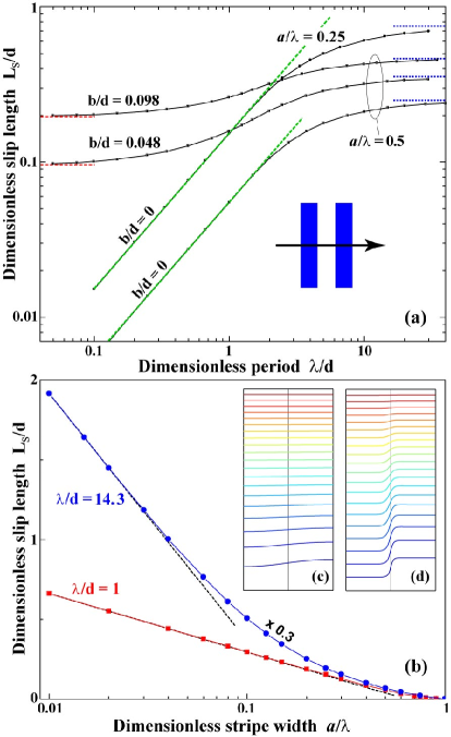
Figure 3: (Color online) (a) Normalized slip length, $L_{s}/d$, versus normalized pattern period, $\lambda/d$, derived from the Stokes solutions for the transverse flow orientation. The parameters values shown are $b/d\!=\!0$, 0.048 and 0.098 and $a/\lambda\!=\!0.25$ and 0.50. The straight lines superimposed on the numerical solutions for $b/d\!=\!0$ correspond to the analytic limit $L_{s}/d\sim\lambda/d$. (b) Normalized slip length $L_{s}/d$ versus normalized stripe width $a/\lambda$ for $\lambda/d\!=\!1$ and 14.3 in the limit $b/d\!=\!0$. The dashed lines correspond to the function $L_{s}/d=A\ln[a/\lambda]+B$, with fitting parameters $A$ and $B$. The data points for the case $\lambda/d\!=\!14.3$ ($A\!=\!-2.245$, $B\!=\!-3.952$) are scaled by a factor 0.3 for convenience. (c-d) Streamlines corresponding to the transverse Stokes flow solutions for (c) $\lambda/d\!=\!1$ and (d) $\lambda/d\!=\!20$ where $b/d\!=\!0.048$ and $a/\lambda\!=\!0.5$. The cell domain size is $\lambda/2\times d$; the thin vertical lines designate the boundary between surfaces of no-shear (left) and finite slip (right).

In the opposite limit $\lambda/d\!\rightarrow\!0$, i.e. where the upper and lower walls are essentially infinitely far apart, the deviation of the flow field from pure shear flow over a homogeneous surface with slip length $L_{s}$ is limited to a thin layer whose thickness scales with $\lambda$. As a consequence, the effective slip length should be independent of the cell depth $d$ and independent of the particular mechanism used to generate the flow, i.e. the same slip length should result for pressure-driven or shear-driven flow. Lauga and Stone Stone03 determined the asymptotic behavior of the effective slip length for pressure-driven flow in a cylindrical tube of radius $R$ with periodically distributed (transverse) rings denoting alternating surfaces of no-shear or no-slip ($b=0$):

$$\lim_{\begin{subarray}{c}b/R=0\\ \lambda/d\rightarrow 0\end{subarray}}\frac{L_{s}}{R}=\frac{\lambda}{2\pi R}\,\ln\!\left(\frac{1}{\cos\left(\frac{\pi}{2}\frac{\lambda-a}{\lambda}\right)}\right)~{}.$$ (31)

The solutions to Eq. (31), obtained by replacing the capillary radius $R$ with the cell depth $d$, superimpose perfectly (sloped dashed lines) onto the full numerical solutions shown in Fig. 3(a). In this limit, the slip length increases linearly with $\lambda/d$ up to a limit $\lambda/d\approx 1$.

The effective slip length in the limit $\lambda/d\!\rightarrow\!0$ for the case $b\!\neq\!0$ can be derived as follows. When the array period $\lambda$ is much smaller than the local slip length $b$, the slip velocity $u(x,z\!=\!0)$ should saturate towards a constant value, $u_{s0}$, over the entire interval $0\leq x\leq\lambda/2$. Since $u(z\!=\!0)\!=\!bu_{z}(z\!=\!0)$, it is also expected that the velocity gradient, $u_{z}(z\!=\!0)$, will assume a constant value in the region $[\lambda-a)/2\leq x\leq\lambda/2,z=0]$. Consequently,

$$\frac{\partial\langle u\rangle}{\partial z}(0)=\frac{u_{s0}}{L_{s}}=\frac{\lambda\!-\!a}{\lambda}\,0\,+\frac{a}{\lambda}\frac{u_{s0}}{b}\ \ \ \Rightarrow\ \ \ \frac{L_{s}}{d}=\frac{\lambda}{a}\frac{b}{d}\,,$$ (32)

i.e. the effective slip length becomes independent of $\lambda/d$ for fixed $a/\lambda$. The term proportional to $(\lambda\!-\!a)/\lambda$ accounts for the vanishing contribution of the no-shear regions to $\partial\langle u\rangle/\partial z(z\!=\!0)$. The horizontal dashed lines shown in Fig. 3(a) for $\lambda/d\!<\!0.1$ represent solutions to Eq. (32) for the designated values of $b/d$ and $a/\lambda$.

In Fig. 3(b) is plotted the effective slip length, $L_{s}/d$, versus $a/\lambda$ for $b/d\!=\!0$ and $\lambda/d\!=\!1.0$ and $14.3$. The data points for $\lambda/d\!=\!14.3$ are scaled by a factor 0.3 for convenience. The effective slip vanishes as $a/\lambda\!\rightarrow\!1$ since the surface coverage by regions of perfect slip decreases to zero. The numerical results were compared to a Taylor expansion of Eq. (31) in the limit of $a/\lambda\!\rightarrow\!0$

$$\frac{L_{s}}{d}=-\frac{\lambda}{2\pi d}\left[\ln\!\left(\frac{a}{\lambda}\right)+\ln\!\left(\frac{\pi}{2}\right)\right].$$ (33)

The dashed line shown in Fig. 3(b) for $\lambda/d\!=\!1.0$ perfectly superimposes on the results of the full numerical solutions. The numerical solution for $\lambda/d\!=\!14.3$ can also be approximated by a fit-function $A\log[a/\lambda]+B$ for $a/\lambda\ll 1$, as shown by the dashed line; however, Eq. (33) no longer holds because $\lambda/d\nleq 1$.

Streamlines of the flow field, corresponding to the contour lines (i.e. constant values) of the streamfunction, are shown in Figs. 3(c,d). The left and right panels represent the solutions for $b/d\!=\!0.048$ and $a/\lambda\!=\!0.5$ for (c) $\lambda/d\!=\!1$ and (d) 20. The vertical line denotes the transition in boundary condition at the lower wall from no-shear (left) to finite slip (right). For small values of $\lambda/d\!\leq\!1.0$, the streamlines are essentially horizontal in the larger portion of the cell and the deviation of the streamfunction from pure Couette flow over a homogeneous surface is confined to a small distance from the patterned wall. As $\lambda/d$ increases, the perturbation extends further away from the lower boundary. For large $\lambda/d$ the streamlines are horizontal above the individual stripes except for a step-like vertical displacement in the vicinity of the transition point $x=(\lambda\!-\!a)/2$.

II.2 Longitudinal configuration

The velocity field corresponding to the longitudinal configuration shown in Fig. 1(b) is unidirectional and given by ${\bf u}(x,z)\!=\!(0,v,0)$. There is no pressure gradient in this configuration and the numerical solutions are derived directly from the Stokes equation $\nabla^{2}v\!=\!0$. The computational cell is shown in Fig. 2(b), where the direction of motion of the upper wall is indicated by the white concentric circles. Only four BCs are required for solution of the velocity field $v$. Aside from the obvious constraints of finite slip, $v_{x}$ must vanish at $x\!=\!0$ and $x\!=\!\lambda/2$ because these are planes of mirror symmetry. The complete set of BCs is given by:

$$v\left(\mbox{$0\!\leq\!x\!\leq\!\frac{\lambda}{2}$},z\!=\!d\right) = U\!-\!bv_{z}(x,z\!=\!d)$$ (34)

$$v_{z}\left(\mbox{$0\!\leq\!x\!\leq\!\frac{\lambda-a}{2}$},z\!=\!0\right) = 0$$ (35)

$$v\left(\mbox{$\frac{\lambda-a}{2}\!\leq\!x\!\leq\!\frac{\lambda}{2}$},z\!=\!0\right) = bv_{z}(x,z\!=\!0)$$ (36)

$$v_{x}(x\!=\!0,z) = 0\ =\ v_{x}\left(\mbox{$\frac{\lambda}{2}$},z\right)~{}.$$ (37)

Eq. (37) and a lateral average of the Stokes equation across the computational cell i.e. $\langle v(z)\rangle=(2/\lambda)\int_{0}^{\lambda/2}v(x,z)\,dx$, leads to $\langle v\rangle_{zz}\!=\!0$. As in the transverse case, the averaged velocity profile, $\langle v\rangle$, is therefore a linear function of $z$. Geometric similarity determines the equation for the effective slip length, namely

$$\frac{L_{s}}{d}=\frac{\langle v(z\!=\!0)\rangle}{\langle v(z\!=\!d)\rangle-\langle v(z\!=\!0)\rangle}~{}.$$ (38)

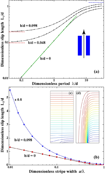
Figure 4: (Color online) (a) Normalized slip length $L_{s}/d$ versus normalized pattern period $\lambda/d$ derived from the Stokes solutions for the longitudinal flow orientation. The parameter values shown are $b/d\!=\!0$, 0.048 and 0.098 and $a/\lambda\!=\!0.5$. The straight line superimposed on the data for $b/d\!=\!0$ corresponds to Eq. (39) where $L_{s}/d\!\sim\!\lambda/d$. (b) Normalized slip length $L_{s}/d$ versus normalized stripe width $a/\lambda$ for $\lambda/d\!=\!1$ and $b/d\!=\!0$ and 0.098. The straight line superimposed on the numerical solutions corresponds to Eq. (41). The data points for $b/d\!=\!0.098$ are scaled by a factor 0.5 for convenience. (c-d) Velocity contours corresponding to the longitudinal Stokes flow solutions for (c) $\lambda/d\!=\!0.35$ and (d) 10, where $b/d\!=\!0.048$ and $a/\lambda\!=\!0.5$. The domain size is $\lambda/2\times d$; the thin vertical lines designate the boundary between surfaces of no-shear (left) and finite slip (right).

Figure 4(a) represents numerical results for the normalized effective slip length, $L_{s}/d$, as a function of $\lambda/d$. Over the range shown, $L_{s}/d$ increases monotonically with $\lambda/d$. As with the transverse geometry, there is no significant increase in slip length beyond $\lambda/d\sim{\cal O}(10)$. The absolute values of $L_{s}/d$ are larger than in the transverse case. This is due to the fact that for unidirectional flow, the liquid above the region of no-shear always remains in line with the frictionless stripes and is never subject to any deceleration caused by the regions of finite slip. The functional dependence of $L_{s}/d$ on $\lambda/d$, however, is identical to the transverse orientation. As $\lambda/d\!\rightarrow\!0$, the slip length should be independent of the cell depth, $d$, and independent of the type of flow (whether pressure- or shear-driven). Using the analytical solutions of Philip Philip1 ; Philip2 for the longitudinal configuration, Lauga and Stone Stone03 extracted the effective slip length for pressure driven flow in a cylindrical tube of radius $R$ in the presence of alternating stripes of no-shear and no-slip ($b\!=\!0$):

$$\lim_{\begin{subarray}{c}b/R=0\\ \lambda/R\rightarrow 0\end{subarray}}\frac{L_{s}}{R}=\frac{\lambda}{\pi R}\ln\!\left(\frac{1}{\cos\left(\frac{\lambda-a}{\lambda}\frac{\pi}{2}\right)}\right)~{}.$$ (39)

The solutions to Eq. (39), obtained by replacing the capillary radius, $R$, with the planar cell depth, $d$, are almost indistinguishable from the results of the full numerical solutions in Fig. 4(a). In this limit, the slip length $L_{s}/d$ is exactly twice that of the transverse configuration [see Eq. (31)] and scales linearly with $\lambda/d$.

An analytic expression for the effective slip, $L_{s}/d$, can be derived in the limit $\lambda/d\!\rightarrow\!\infty$, by examining the flow field above the patterned substrates. The velocity profile above the no-shear surface (1) is plug-like and given by $v_{1}(z)=U$. Above the surface of finite slip, $v_{2}(z)=U(z+b)/(2b+d)$. The latter result is obtained by noting that the shear rate, $u_{z}$, is constant throughout the gap depth and equal to $U/(2b+d)$. Calculating the average flow speed, $\langle v\rangle$, at the upper and lower boundaries and substituting these into Eq. (38) leads to the expression:

$$\lim_{\lambda/d\rightarrow\infty}\frac{L_{s}}{d}=\frac{\lambda-a}{a}+\frac{2\lambda-a}{a}\,\frac{b}{d}~{}.$$ (40)

The horizontal dashed line for $b/d=0.098$ and $\lambda/d\gtrsim 10$ corresponds to Eq. (40).

In Fig. 4(b) is plotted the numerical solutions for $L_{s}/d$ versus $a/\lambda$ for $\lambda/d\!=\!1$ and $b/d=0~{}\mbox{and}~{}0.098$. The data points for $b/d=0.098$ have been scaled by 0.5 for convenience. For $b/d\!=\!0$ and small values $a/\lambda$, a Taylor expansion of Eq. (39) gives

$$\lim_{\begin{subarray}{c}b/d=0\\ \lambda/d\rightarrow 0\end{subarray}}\frac{L_{s}}{d}=-\frac{\lambda}{\pi d}\left[\ln\!\left(\frac{a}{\lambda}\right)+\ln\!\left(\frac{\pi}{2}\right)\right].$$ (41)

The straight line superimposed on the data in Fig. 4(b) represents the asymptotic values given by Eq. (41). The agreement with the analytical limit for $a/\lambda\!\lesssim\!0.3$ is very good.

Velocity contours, corresponding to constant values of $v$, are shown in Figs. 4(c,d). The left and right panels represent solutions for (c) $\lambda/d\!=\!0.35$ and (d) $\lambda/d\!=\!10$ where $b/d\!=\!0.048$ and $a/\lambda\!=\!0.5$. The vertical line denotes the position corresponding to the change in boundary condition at the lower wall from no-shear (left) to finite slip (right). For $\lambda/d\!\leq\!0.35$, the velocity contours are horizontal throughout almost the entire cell and the deviations from pure shear flow over a homogeneous surface are confined to a small distance from the patterned wall. For $\lambda/d\!=\!10$, the perturbation extends vertically across the cell. For large $\lambda/d$, the velocity distribution varies from plug–like above the region of perfect slip to Couette–like above the region of finite slip, as assumed in the derivation leading to Eq. (40) for $\lambda/d\rightarrow\infty$.

III MD simulations and parameter values

We have previously used MD simulations to investigate what equilibrium parameters control the degree of slip in simple and polymeric fluids and how the slip length depends on shear rate Nature97 ; Priezjev04 . In these previous studies, the wall–fluid potential was spatially homogeneous. In this current work, we examine the behavior of the effective slip length for a fluid subject to planar shear in the presence of a heterogeneous bottom wall for the two flow configurations shown in Fig. 1. The wall–fluid interactions are adjusted to mimic alternating stripes of finite slip and no–shear by adjusting the attractive part of the potential to simulate more attractive and less attractive regions. The MD simulations described next were conducted with the LAMMPS numerical code Lammps . In what follows, we refer to the more attractive surface as wetting and the less attractive surface as non–wetting.

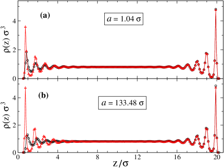
Figure 5: (Color online) Average normalized fluid density, $\rho(z)\sigma^{3}$, above the wetting ($\delta_{\rm wf}\!\!=\!1.0$: triangles) and non–wetting stripes ($\delta_{\rm wf}\!\!=\!0.1$: circles). The parameter values shown are (a) $a\!=\!1.04\,\sigma$ and (b) $a\!=\!133.48\,\sigma$ for $\varepsilon_{\rm wf}/\varepsilon\!=\!0.8$.

The simulation cell consisted of $30720$ fluid molecules interacting through a Lennard–Jones (LJ) potential,

$$V_{LJ}(r)=4\varepsilon\bigg{[}\bigg{(}\frac{\sigma}{r}\bigg{)}^{12}-\delta~{}\bigg{(}\frac{\sigma}{r}\bigg{)}^{6}~{}\bigg{]}~{},$$ (42)

where $\varepsilon$ and $\sigma$ represent the energy and length scales characteristic of the fluid phase. The cut-off radius was set to $r_{c}\!=\!2.5\,\sigma$. The parameter $\delta$, which controls the attractive part of the potential for fluid–fluid interactions, was held fixed at $\delta\!=\!1$. The wall–fluid (wf) parameters were chosen to be $\sigma_{\rm wf}\!=\!0.75\,\sigma$ and $\varepsilon_{\rm wf}/\varepsilon\!=\!0.8$, 0.9 or 1.0. Surfaces of finite slip in the hydrodynamic analysis corresponded to the parameter value $\delta_{\rm wf}\!=\!1.0$ (i.e. wetting); surfaces of no-shear (or likewise perfect slip) corresponded to the value $\delta_{\rm wf}\!=\!0.1$ (i.e. non-wetting). For the MD simulations, we restricted our study to the case $a/\lambda\!=\!1/2$ such that the wetting and non-wetting portions of the substrate occupy equal areas.

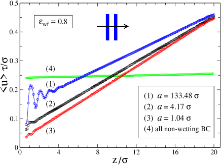
Figure 6: (Color online) Average normalized velocity profile, $\langle u\rangle\,\tau/\sigma$ corresponding to the transverse flow configuration for $\varepsilon_{\rm wf}/\varepsilon\!=\!0.8$ and $a/\sigma=1.04$, 4.17 and 133.48. The nearly horizontal profile shown in (4), which designates a plug-like profile representative of surfaces with large slip lengths, was obtained by setting the wall-fluid potential parameter to $\delta_{\rm wf}=0.1$ along both walls. This choice effectively reproduces non-wetting bounding walls.

The upper and lower walls of the simulation cell each consisted of $12288$ molecules distributed between two (111) planes of an FCC lattice with density $\rho_{w}\!=\!4\rho$, where $\rho\!=\!0.81\,\sigma^{-3}$ is the density of the fluid phase. The fluid was confined to a fixed height $d=20.15\,\sigma$; the cell volume was $266.96\,\sigma\times 7.22\,\sigma\times d$ for the transverse geometry. To eliminate any finite size effects for the longitudinal geometry, the system size along the $\hat{y}$-axis was doubled in length to $14.45\,\sigma$, requiring simulations with $61440$ fluid molecules. For either configuration, periodic BCs were enforced along the $\hat{x}$ and $\hat{y}$ axes. The fluid was held at a constant temperature $T\!=\!1.1\,\varepsilon/k_{B}$ by means of a Langevin thermostat Grest86 with a friction coefficient $\tau^{-1}$. Here, $k_{B}$ is the Boltzmann constant. This damping term is only applied to the coordinate equation perpendicular to the direction of flow Thompson90 ; Nature97 . The equations of motion were integrated using the Verlet algorithm Allen87 with a time step $\triangle t\!=\!0.005\,\tau$, where $\tau\!=\!\sqrt{m\sigma^{2}/\varepsilon}$ represents the characteristic time set by the LJ potential and $m$ is the monomer mass. The fluid was subject to steady planar shear by translating the upper wall at a constant speed $U$; the lower, patterned wall remained stationary. In all the simulations, the speed of the upper wall was held fixed at $U=0.5\,\sigma/\tau$. After an equilibration period exceeding $10^{4}\tau$, the fluid velocity profile was obtained by averaging the instantaneous monomer speeds in slices $\Delta z=0.1\,\sigma$ for a time interval $\Delta t\approx 3\cdot 10^{4}\tau$. The Reynolds number, based on the upper wall speed $U$, the wall separation $d$ and the fluid shear viscosity (determined previously Nature97 ; Priezjev04 to be $\mu=2.2\pm 0.2\epsilon\tau/\sigma^{3}$ for comparable shear rates) was estimated to range from $2\!-\!5$, indicative of negligible inertial effects and laminar flow conditions. In fact, this estimate provides only an upper bound on the Reynolds number, since the actual fluid velocity for surfaces comprising regions of finite and infinite slip is significantly smaller than the upper wall speed. In our studies, use of the fluid flow speed further reduces ${\sf Re}$ by a factor of up to 2. We conclude that the small Reynolds numbers characterizing the MD simulations are consistent with the theoretical restriction for the Stokes flow solutions obtained in the limit ${\sf Re}\!=\!0$. We also note that the numerical solutions to the Stokes equation for the longitudinal geometry are valid irrespective of the value of the Reynolds number because the unidirectional flow causes the inertial term in the Navier-Stokes equation to vanish identically.

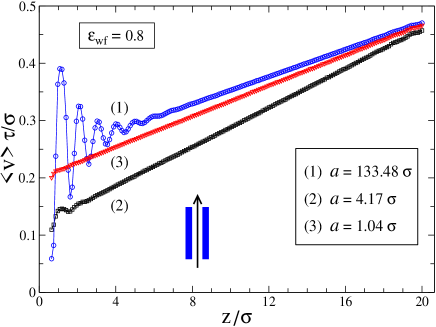
Figure 7: (Color online) Average normalized velocity profile, $\langle v\rangle\,\tau/\sigma$, corresponding to the longitudinal flow configuration for $\varepsilon_{\rm wf}/\varepsilon\!=\!0.8$ and $a/\sigma=1.04$, 4.17 and 133.48.

IV Results of MD simulations for Transverse and Longitudinal Flow

The two sets of curves in Fig. 5 show the average normalized fluid density, $\rho(z)\sigma^{3}$, for the transverse flow configuration in the region above the wetting and non–wetting stripes for $\varepsilon_{\rm wf}/\varepsilon\!=\!0.8$ and $a/\sigma=1.04~{}\mbox{and}~{}133.48$. The choice $a\!=\!133.48\,\sigma$ represents the accommodation of only two stripes at the lower wall within the Couette cell. The oscillations near the upper and lower boundaries reflect the molecular layering caused by the presence of dense walls  Thompson90 . Increasing the attractive part of the LJ potential generates larger peak maxima and more oscillations. Above either type surface, the density oscillations persist for about $4-6$ molecular diameters from the wall. Decreasing the strength of the attractive interaction shifts the first peak maximum away from the lower wall. Also, the fluid density above the wetting stripes is found to increase with $a/\sigma$. The density profiles corresponding to longitudinal flow configurations are quite similar to the ones shown here.

Figure 6 shows representative velocity profiles across the cell depth for transverse flow with $\varepsilon_{\rm wf}/\varepsilon\!=\!0.8$ and $a/\sigma=1.04,~{}4.17~{}\mbox{and}~{}133.48$. Shown for comparison is the velocity profile corresponding to the case of uniformly non-wetting walls where $\delta_{\rm wf}=0.1$ holds for both surfaces. Decreasing the wall–fluid interaction leads to a high degree of slip and a plug–like velocity field. The remaining three profiles increase linearly with $z/\sigma$, as expected for a fluid subject to planar shear, except in the vicinity of the lower wall. Significant deviations from linearity occur for large stripe widths. These oscillations are caused by the difference in the positions of the fluid density maxima above the wetting and non–wetting regions [see Fig. 5(b)]. As evident from the velocity profile, the degree of slip increases with increasing values of $a$.

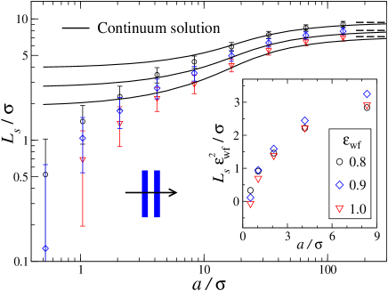
Figure 8: (Color online) Comparison of the effective slip length, $L_{s}$, as extracted from the MD simulations (symbols), with numerical solutions of the Stokes equation (continuous lines) for transverse flow. The local slip length, $b$, as extracted from the MD simulations, decreases with increasing wall–fluid attraction energy, namely $b/\sigma\!=\!1.97$, 1.36 and 0.95 for $\varepsilon_{\rm wf}/\varepsilon\!=\!0.8$ ($\circ$), 0.9 ($\diamond$) and 1.0 ($\triangledown$), respectively. The dashed horizontal lines for $a/\sigma\gtrsim 100$ correspond to Eq. (30). Inset: MD results showing collapse of the effective slip length $L_{s}/\sigma$ when rescaled by the quantity ${\varepsilon}^{2}_{\rm wf}$, versus $a/\sigma$.

Figure 7 shows the computed velocity profiles for longitudinal configurations. The behavior is similar to that shown in Fig. 6 for the transverse orientation, but the amplitude of the oscillations near the lower wall is significantly larger. In this case, the degree of slip does not increase monotonically with $a$. The smallest stripe width generates the second largest slip velocity in Fig. 7. As the stripe width increases, it is found that the wetting regions induce stronger molecular ordering in the first fluid layer adjacent to the wall, causing a reduction in the slip length, as noted in Fig. 10.

For direct comparison to the hydrodynamic predictions, it was necessary to extract the actual values of the local slip length, $b$, representative of the surfaces characterized by $\delta_{\rm wf}=1.0$, for input values to the boundary conditions used in computing the solutions to the Stokes equation. This was accomplished in the MD simulations by extrapolating the average velocity profile at the top wall to a speed $U$ for different values of $a$ imposed on the lower wall. The extrapolated distance $b$ was found to depend on the wall–fluid interaction energy but not the shear rate in the fluid nor the flow orientation. As expected, the values of $b$ decreased with increasing value of the wall–fluid interaction energy, namely $b/\sigma\!=\!1.97$, 1.36 and 0.95 for $\varepsilon_{\rm wf}/\varepsilon\!=\!0.8$, 0.9 and 1.0, respectively. By contrast, the local slip length for the flat velocity profile shown in Fig. 6 for uniformly non-wetting walls was found to be $(362\pm 10)\,\sigma$. Given that this slip length significantly exceeds the wall separation, the choice $\delta_{\rm wf}\!=\!0.1$ approximates very well the behavior of surfaces of perfect slip (i.e. no–shear) assumed in the continuum calculations.

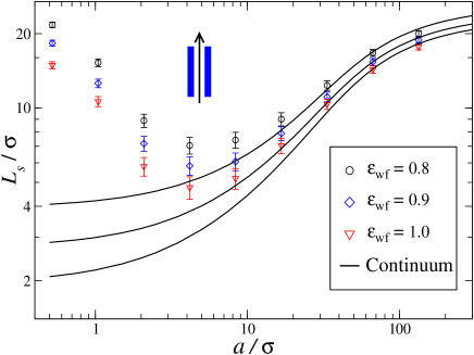
Figure 9: (Color online) Direct comparison of the effective slip length extracted from the MD simulations (symbols) with the numerical solutions of the Stokes equation (continuous lines) for longitudinal flow. The local slip length, $b$, as extracted from the MD simulations, varies with the LJ wall–fluid interaction energy, $\varepsilon_{\rm wf}$ as $b/\sigma\!=\!1.97$, 1.36 and 0.95 for $\varepsilon_{\rm wf}/\varepsilon\!=\!0.8$ ($\circ$), 0.9 ($\diamond$) and 1.0 ($\triangledown$), respectively. The local slip lengths are observed to be independent of the flow orientation.

The composite or effective slip length, $L_{s}$, was determined in the MD simulations by linear extrapolation below the stationary lower surface of the velocity profile to the value zero. Figure 8 represents a plot of $L_{s}/\sigma$ with increasing normalized stripe width, $a/\sigma$, and increasing wall–fluid interaction strength, $\varepsilon_{\rm wf}$, for transverse flow configurations. The MD results (symbols) show a sharp increase in slip length for $a/\sigma\lesssim 10$ and saturation to a constant value beyond $a/\sigma\gtrsim 100$.

V Discussion

As described in Section II.1 and for fixed values of $a/\lambda$, the effective slip length derived from hydrodynamic considerations depends only on the ratios $\lambda/d$ and $b/d$. The molecular length scale, $\sigma$, plays no part in the analysis. For direct comparison to the MD results, it was therefore necessary to multiply the numerical values of $L_{s}/d$, $\lambda/d$ and $b/d$ from the Stokes solutions with the value of the wall separation, $d\!=\!20.15\,\sigma$, used in the MD simulations. The largest ratio, $a/d\!=\!6.62$, accessible to the MD simulations was only limited by computational resources. The solid lines shown in Fig. 8 represent solutions of the Stokes flow equation for transverse flow, as discussed in Section II.1. The agreement between the continuum predictions and the MD simulations is excellent for $a/\sigma\gtrsim{\cal O}(10)$; significant deviations occur for $a/\sigma\lesssim{\cal O}(1)$. The asymptotic predictions given by Eq. (30) for $\lambda/d\!=\!2a/d\!\rightarrow\!\infty$ are designated by the dashed horizontal lines in Fig. 8.

The Green-Kubo type analysis of Barrat and Bocquet Barrat94 ; Barrat99 for homogeneous surfaces characterized by a single wall–fluid interaction energy predicts that the slip length scales as $\varepsilon_{\rm wf}^{-2}$ provided the in–plane structure factor, fluid contact density, and in–plane diffusion coefficient characteristic of the first fluid layer remain relatively constant. The results shown in the inset of Fig. 8 for the transverse geometry confirm this prediction for the range $a\lesssim 10\,\sigma$, even for the case of a composite potential where the wall–fluid interaction alternates between two values of $\delta_{\rm wf}$. This collapse fails above $a\!\gtrsim\!10\,\sigma$ where the continuum solutions show excellent agreement with the molecular simulations. This behavior suggests that for $a/\sigma\!\lesssim\!{\cal O}(10)$, the effective slip length is mostly determined by the molecular scale frictional properties between the first fluid layer and the lower wall. For $a/\sigma\!\gtrsim\!{\cal O}(10)$, however, the effective slip length is set by the wall separation $d$, the pattern lengthscales $a$ and $\lambda$ and the local slip length $b$. The transition region $8\lesssim a/\sigma\lesssim 30$ therefore contains mesoscopic information from both the molecular and hydrodynamic descriptions.

The deviation between the MD simulations and the Stokes solutions below $a/\sigma\!\lesssim\!{\cal O}(10)$ can be understood as follows. The lower wall is comprised of a potential whose interaction strength alternates between wetting and non–wetting values with a periodicity set by the stripe width $a$, which approaches the molecular scale. The fluid molecules no longer experience uninterrupted stretches of wetting and non-wetting regions; instead, the fluid molecules are exposed to an effectively roughened surface with molecular scale corrugations. These corrugations trap the fluid molecules, thereby suppressing slip at the wall–fluid interface. The commensurability between the fluid molecular size and the wall corrugation size can in fact lead to a no-slip condition for slightly larger values of $\varepsilon_{\rm wf}$ Priezjev05 . It is therefore not surprising that the effective slip length for the transverse configuration, as shown in Fig. 8, decreases sharply with decreasing values of $a$. This effect also explains why for the smallest values of $a$ the slip length $L_{s}$ is even smaller smaller than the local slip length obtained for a fluid confined between two identical walls both characterized by the same value $\delta_{\rm wf}=1.0$. For example, for $\varepsilon_{\rm wf}/\varepsilon=0.8$ and $a/\sigma\!=\!1.04$, we find that $b/\sigma\!=\!1.97$ but $L_{s}/\sigma\!=\!0.5$!

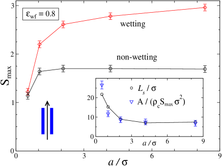
Figure 10: (Color online) The dominant peak in the in–plane fluid structure factor evaluated separately above the wetting ($\diamond$) and non–wetting ($\circ$) regions for longitudinal flow and $\varepsilon_{\rm wf}/\varepsilon\!=\!0.8$. Inset: MD results showing the strong correlation between the effective slip length $L_{s}/\sigma$ (circles: data from Fig. 9) and the quantity $A(S_{\max}\rho_{c}\sigma^{2})^{-1}$ (triangles), which characterizes the degree of molecular ordering within the first fluid layer above the wetting stripes. The value of the fitting parameter $A$ is 92.4.

Figure 9 shows the behavior of $L_{s}/\sigma$ as a function of stripe width, $a/\sigma$, and increasing interaction strength, $\varepsilon_{\rm wf}$, for longitudinal flow configurations. The results of the MD simulations (symbols) show a sharp decrease in slip length below $a/\sigma\!\sim\!10$ followed by a rapid rise. The effective slip lengths have similar magnitudes for very small and very large values of $a$. Once again, there is excellent agreement between the Stokes flow solutions and the MD simulations for $a/\sigma\!\gtrsim\!{\cal O}(10)$ but strong deviations below this value. In contrast to the transverse configuration, however, the MD results predict much larger effective slips than the continuum solutions for $a/\sigma\lesssim{\cal O}(10)$. Because of the translational invariance of the flow inherent in this case, the molecular scale roughness set by the composite potential at the bottom wall cannot diminish the slip length. The reduction in molecular ordering above the wetting regions with decreasing stripe width, however, leads to an increase in the slip length which exceeds the slip lengths obtained for the transverse configuration as well as the continuum predictions.

Previous MD simulations of Newtonian and non-Newtonian fluids have demonstrated that the slip length for surfaces characterized by a single wall–fluid potential correlates strongly with the degree of molecular ordering in the first fluid layer adjacent to the wall Thompson90 ; Thompson92 ; Thompson95 ; Barrat94 ; Nature97 ; Barrat99 ; Priezjev04 . The more orderly the molecular organization, as reflected by the maximum value of the in-plane structure function, $S_{\max}$, the smaller the slip length. To test these predictions for the case of patterned walls in a longitudinal orientation, we computed the maximum value of the in-plane structure function within the first fluid layer above the wetting and non-wetting regions separately. The thickness of the first fluid layer was estimated from the position of the first minimum in the density profile above a wetting stripe. The contact density $\rho_{c}$ was identified with the maximum of the fluid density within the first fluid layer. The structure function was computed according to $S(q)\!\!=\!|\sum_{1}^{N_{\ell}}e^{iqy}|^{2}/N_{\ell}$, where $N_{\ell}$ is the number of molecules in the first fluid layer adjacent to either a wetting or non–wetting surface. As shown in Fig. 10, the molecular ordering adjacent to a wetting region is far stronger and increases with increasing stripe width, $a$. By contrast, the molecular ordering adjacent to the non–wetting region is unaffected by the stripe width, $a$, except for the smallest value shown. The inset in Fig. 10 demonstrates the correlation between the effective length and the parameter $(S_{\max}\rho_{c}\sigma^{2})^{-1}$ as estimated above the wetting regions. Here, the values of $L_{s}/\sigma$ versus $a/\sigma$ from Fig. 9 are plotted alongside the quantity $A\,(S_{\max}\rho_{c}\sigma^{2})^{-1}$, where $A\!=\!92.4$ is a fitting parameter. In the limit $a/\sigma\!\lesssim\!{\cal O}(10)$, the strong correlation between $L_{s}$ and $A\,(S_{\max}\rho_{c}\sigma^{2})^{-1}$ establishes that the increase in effective slip length for narrow stripe widths is mainly caused by the reduction in molecular ordering within the first fluid layer above the wetting zones.

The BCs used in the continuum analysis correspond to stripes of finite (or no) slip and no shear (i.e. $b=\infty$). We repeated the analysis in Section II by replacing the no-shear BC with a second slip BC to define surfaces comprising alternating stripes of small ($b/\sigma=1.97$) and large slip ($b/\sigma=362$, as extracted from case (4) shown in Fig. 6). For the transverse configuration, the curve corresponding to $b/\sigma=1.97$ in Fig. 8 showed a slight decrease in $L_{s}$ of about 3% for $a/\sigma>30$, whereas the longitudinal configuration generated a decrease of up to 9% with respect to the values shown in Fig. 9.

VI Summary

We have investigated the behavior of the slip length in Newtonian liquids subject to planar shear in a Couette cell with mixed surface boundary conditions. The upper wall is modelled as a homogenous surface with finite or no-slip moving at a constant speed above a lower stationary wall patterned with alternating stripes representing regions of no-shear and finite or no-slip. The velocity fields and effective slip lengths are computed both from molecular dynamics (MD) simulations and solution of the Stokes equation for flow parallel (longitudinal case) or perpendicular (transverse case) to the stripe pattern. Detailed comparison between the results of the hydrodynamic calculations and MD simulations shows excellent agreement when the length scale of the substrate pattern geometry is larger than ${\cal O}(10\,\sigma)$, where $\sigma$ denotes the fluid molecular diameter as set by the Lennard-Jones interaction. The effective slip length then increases monotonically with $a/\sigma$ to a saturation value. For the transverse case, the Stokes flow solutions predict an effective slip larger than the MD results when $a/\sigma\sim{\cal O}(10)$. This discrepancy is understood from a molecular point of view since a narrowing of the regions subject either to no-shear or no-slip essentially establishes a roughened surface. The molecular scale corrugation created by the composite wall potential strongly reduces the effective slip length below the hydrodynamic results. This surface roughening effect is not present for the longitudinal flow configuration since the fluid molecules are transported along homogeneous stripes representing regions of either no-shear or finite slip. In this case, however, the 2D fluid structure factor above the non-wetting stripes (regions of perfect slip or equivalently no-shear) decreases for $a/\sigma\lesssim{\cal O}(10)$, which enhances the effective slip lengths above the values predicted by the hydrodynamic solutions. On the molecular level, the strong correlation observed between the effective slip length and the product $(\rho_{c}S_{\rm max})^{-1}$ confirms that a reduction in molecular ordering within the first fluid layer generates an increase in the effective slip length.

Detailed comparison between continuum computations and molecular dynamics simulations is of increasing importance to the development of hybrid computational schemes Thompson ; Hadjiconstantinou ; Feder ; Nie04 . These algorithms are designed to stitch together hydrodynamic solutions obtained from continuum equations with the molecular scale solutions obtained from MD simulations or other microscopic solvers. It has been demonstrated that the spatial coupling across this wide range in length scales can be achieved by implementation of constraint dynamics within an overlap region. We hope that our studies of shear driven flow along surfaces with mixed boundary conditions will complement ongoing efforts using hybrid codes. The system and results described here offer an interesting test case for better understanding of the intermediate region bridging the behavior of fluids from the nanoscale to microscale dimensions.

- (1) A. A. Darhuber and S. M. Troian, Annu. Rev. Fluid Mech. 37, 425 (2005).
- (2) E. Schnell, J. Appl. Phys. 27, 1149 (1956).
- (3) J. Baudry, É. Charlaix, A. Tonck and D. Mazuyer, Langmuir 17, 5232 (2001).
- (4) D. C. Tretheway and C. D. Meinhart, Phys. Fluids 14, L9 (2002).
- (5) C. H. Choi, K. J. A. Westin, and K. S. Breuer, Phys. Fluids 15, 2897 (2003).
- (6) K. Watanabe, Y. Udagawa, and H. Udagawa, J. Fluid Mech. 381, 225 (1999).
- (7) C. Cottin-Bizonne, J.-L. Barrat, L. Bocquet, and É. Charlaix, Nature Mater. 2, 237 (2003).
- (8) T. N. Krupenkin, J. A. Taylor, T. M. Schneider, and S. Yang, Langmuir 20, 3824 (2004).
- (9) N. Ishida, T. Inoue, M. Miyahara, and K. Higashitani, Langmuir 16, 6377 (2000).
- (10) J. W. G. Tyrrell and P. Attard, Phys. Rev. Lett. 87, 176104 (2001).
- (11) R. Steitz, T. Gutberlet, T. Hauss, B. Klösgen, R. Krastev, S. Schemmel, A. C. Simonsen, and G. H. Findenegg, Langmuir 19, 2409 (2003).
- (12) L. Léger, H. Hervet, G. Massey, and E. Durliat, J. Phys.: Condens. Matter 9, 7719 (1997).
- (13) H. Hervet and L. Léger, C. R. Physique 4, 241 (2003).
- (14) M. M. Denn, Annu. Rev. Fluid Mech. 33, 265 (2001).
- (15) F. Brochard-Wyart, P. G. de Gennes, and S. M. Troian, C. R. Acad. Sci. Paris, 310, Serie II, 1169 (1990).
- (16) C. L. M. H. Navier, Mem. Acad. Roy. Sci. Inst. France 6, 839 (1827).
- (17) O. I. Vinogradova, Int. J. Miner. Process. 56, 31 (1999).
- (18) S. Richardson, J. Fluid Mech. 59, 707 (1973).
- (19) L. M. Hocking, J. Fluid Mech. 76, 801 (1976).
- (20) K. M. Jansons, Phys. Fluids 31, 15 (1988).
- (21) D. Einzel, P. Panzer, and M. Liu, Phys. Rev. Lett. 64, 2269 (1990).
- (22) M. J. Miksis and S. H. Davis, J. Fluid Mech. 273, 125 (1994).
- (23) L. Bocquet and J.-L. Barrat, Phys. Rev. E 49, 3079 (1994).
- (24) H. A. Barnes, J. Non-Newtonian Fluid Mech. 56, 221 (1995).
- (25) D. Andrienko B. Dünweg, and O. I. Vinogradova, J. Chem. Phys. 119, 13106 (2003).
- (26) K. B. Migler, H. Hervet, and L. Leger, Phys. Rev. Lett. 70, 287 (1993).
- (27) V. Mhetar and L. A. Archer, Macromol. 31, 8607 (1998); 31, 8617 (1998).
- (28) P. A. Thompson and S. M. Troian, Nature (London) 389, 360 (1997).
- (29) N. V. Priezjev and S. M. Troian, Phys. Rev. Lett. 92, 018302 (2004).
- (30) R. G. Horn, O. I. Vinogradova, M. E. Mackay, and N. Phan-Thien, J. Chem. Phys. 112, 6424 (2000).
- (31) Y. Zhu and S. Granick, Phys. Rev. Lett. 87, 096105 (2001).
- (32) O. I. Vinogradova, N. F. Bunkin, N. V. Churaev, O. A. Kiseleva, A. V. Lobeyev, and B. W. Ninham, J. Colloid Interface Sci. 173, 443 (1995).
- (33) E. Lauga and H. A. Stone, J. Fluid Mech. 489, 55 (2003).
- (34) J. R. Philip, J. Appl. Math. Phys. 23, 353 (1972).
- (35) J. R. Philip, J. Appl. Math. Phys. 23, 960 (1972).
- (36) P. A. Thompson and M. O. Robbins, Phys. Rev. A 41, 6830 (1990).
- (37) P. A. Thompson, G. S. Grest, and M. O. Robbins, Phys. Rev. Lett. 68, 3448 (1992).
- (38) P. A. Thompson, M. O. Robbins, and G. S. Grest, Israel J. Chem. 35, 93 (1995).
- (39) J.-L. Barrat and L. Bocquet, Phys. Rev. Lett. 82, 4671 (1999); Faraday Discuss. 112, 119 (1999).
- (40) L. G. Leal, Laminar Flow and Convective Transport Processes, (Butterworth-Heinemann, Boston, 1992).
- (41) FemLab Multiphysics Modeling Software, COMSOL, Inc., Burlington, MA.
- (42) J. A. Wass, Sci. Comp. Instr. 21 (10), 34 (2004).
- (43) S. J. Plimpton, J. Comp. Phys. 117, 1 (1995); see also URL http://www.cs.sandia.gov/sjplimp/lammps.html.
- (44) G. S. Grest and K. Kremer, Phys. Rev. A 33, R3628 (1986).
- (45) M. P. Allen and D. J. Tildesley, Computer Simulation of Liquids (Clarendon, Oxford, 1987).
- (46) N. V. Priezjev and S. M. Troian, submitted to J. Fluid Mech. (2005).
- (47) S. T. O’Connell and P. A. Thompson, Phys. Rev. E 52, R5792 (1995).
- (48) N. G. Hadjiconstantinou, J. Comput. Phys. 154, 245 (1999).
- (49) E. G. Flekkøy, G. Wagner, and J. Feder, Europhys. Lett. 52, 271 (2000).
- (50) X. B. Nie, S. Y. Chen, W. E, and M. O. Robbins, J. Fluid Mech. 500, 55 (2004).
- (51) C. Cottin-Bizonne, C. Barentin, É. Charlaix, L. Bocquet and J.-L. Barrat, Eur. Phys. J. E 20, 427 (2004).