Geometric nature of the environment-induced Berry phase and geometric dephasing

Abstract

We investigate the geometric phase or Berry phase (BP) acquired by a spin-half which is both subject to a slowly varying magnetic field and weakly-coupled to a dissipative environment (either quantum or classical). We study how this phase is modified by the environment and find that the modification is of a geometric nature. While the original BP (for an isolated system) is the flux of a monopole-field through the loop traversed by the magnetic field, the environment-induced modification of the BP is the flux of a quadrupole-like field. We find that the environment-induced phase is complex, and its imaginary part is a geometric contribution to dephasing. Its sign depends on the direction of the loop. Unlike the BP, this geometric dephasing is gauge invariant for open paths of the magnetic field.

Introduction. The Berry phase (BP) is a fundamental quantum-mechanical phenomenon related to the adiabatic theorem. Berry Berry (1984) showed that the phase acquired by an eigenstate of a slowly varying Hamiltonian $H(t)$ is related to the geometric properties of the loop traversed by $H(t)$. In the presence of dissipation the condition of adiabaticity and the existence of the Berry phase require careful analysis. The widespread criterion of adiabaticity, based on a comparison of the rate of change of the Hamiltonian with the gap in the spectrum should be modified to involve the matrix elements of the system-environment coupling, cf. Whitney and Gefen (2003). Here we study the interplay of the varying field and the dissipation, analyzing the BP in the limiting case of weak system-environment coupling. This analysis is relevant to the recent and proposed experiments to manipulate quantum two-level systems (qubits). Our findings could be tested in solid-state qubits, such as superconducting nanocircuits Nakamura et al. (1999); Vion et al. (2002); Chiorescu et al. (2002); Falci et al. (2000).

Berry Berry (1984) considers a two-level spin-half system in a magnetic field footnote:units , which is varied slowly along a closed path: $H_{\rm spin}=-{\textstyle\frac{1}{2}}{\bf{B}}(t){\bm{\sigma}}$. The rate of the field’s change is characterized by the time to complete the loop, $t_{\rm P}$. In the adiabatic limit, $Bt_{\rm P}\gg 1$, the relative phase acquired by the eigenstates is a sum $\Phi=\oint|{\bf{B}}(t)|dt+\Phi_{\rm BP}$ of the dynamical and Berry phases. The latter is geometric, it depends on the geometry of the loop but not on the details of its traversal (for an isolated spin-half it is given by the solid angle subtended by the loop ${\bf{B}}(t)$). In the spin language, the evolution is a rotation of the spin by an angle $\Phi$ about ${\bf{B}}$.

If the spin is not isolated, the dynamics are more complicated. For a static field, ${\bf{B}}$, dissipation induces energy and phase relaxation processes (with the time-scales $T_{1}$, $T_{2}$ respectively) and a Lamb-like shift of the level splitting, $\delta B_{\rm Lamb}$, which modifies the dynamical phase. Strong dephasing masks the BP, however it can be observed if $B\gg T_{2}^{-1}$ Whitney and Gefen (2003). In this weak-coupling limit one can carry out a BP experiment slowly enough for non-adiabatic effects to be ignored ($t_{\rm P}\gg B^{-1}$) while ensuring it is fast enough that dephasing has not destroyed all phase information ($t_{\rm P}\lesssim T_{2}$).

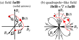
Figure 1: (a) The field $\delta{\bf a}(B)$, see eq. (13), in the vicinity of an open path of ${\bf B}(t)$ (the dotted line). The environment-induced modification of the Berry phase, $\delta\Phi_{\rm BP}$, is the integral of $\delta{\bf a}(B)$ along this path. For such open-paths, the geometric dephasing is gauge-invariant (unlike the phase). (b) The quadrupole-like field $\delta{\bf b}(B)$, see eqs. (14-15), ($\delta{\bf b}(B)$ is cylindrically symmetric about the $B_{z}$-axis). For a closed path of ${\bf B}(t)$, $\delta\Phi_{\rm BP}$ is given by the flux of $\delta{\bf b}(B)$ through the path.

In this letter we show that the coupling to the environment modifies the BP when the magnetic field is slowly varied. In the adiabatic limit this modification, $\delta\Phi_{\rm BP}$, is geometric (see Fig. 1) and complex Garrison and Wright (1988). Its real part is an environment-induced BP, thus the total BP is $\Phi_{\rm BP}^{(0)}+{\rm Re}[\delta\Phi_{\rm BP}]$ (where $\Phi_{\rm BP}^{(0)}$ is the BP for an isolated spin-half). Its imaginary part, ${\rm Im}[\delta\Phi_{\rm BP}]$, is a geometric correction to dephasing, whose sign depends on the direction of the loop. The magnitude of coherency will thus depend on the sign of the loop’s winding number. Notably ${\rm Im}[\delta\Phi_{\rm BP}]$ is gauge-invariant for open as well as closed paths of the $B$-field.

Specifically we study the environment-induced BP for an arbitrary path ${\bf{B}}(t)$, allowing us to analyze its geometric nature. For an isolated spin-half the Berry phase is given by the flux through the closed loop ${\bf{B}}(t)$ of the field ${\bf{b}}_{\rm m}({\bf{B}})$ of a charge-one monopole at the origin in ${\bf{B}}$-space Berry (1984): we show that the environment-induced modification may be interpreted similarly and find the corresponding field distribution $\delta{\bf{b}}({\bf{B}})$ in the ${\bf{B}}$-space. This field (and thus $\delta\Phi_{\rm BP}$) scales quadratically with the spin-environment coupling, similarly to the dissipative rates, $T_{1}^{-1}$, $T_{2}^{-1}$. If the environment-induced field fluctuates along a single direction, $z$, the field $\delta{\bf{b}}({\bf{B}})$ is axially symmetric, has no axial component, $\delta b_{\varphi}=0$, and the angular distribution of a quadrupole. The field $\delta{\bf{b}}({\bf{B}})$ is given by a sum over frequencies of the environment modes (for the lowest non-trivial order in the strength of the spin-environment coupling). The contribution of low frequencies $\Omega\ll B$ to $\delta{\bf{b}}$ is exactly the field of a quadrupole, while high-frequency modes have the angular dependence of a quadrupole but a different radial dependence.

Let us emphasize the novel points of our analysis in comparison to earlier work on BP in systems coupled to quantum or classical environments Whitney and Gefen (2003); see e.g. D. Ellinas et al. (1989); Gaitan (1998); DeChiaraPalma . Some of these works have focused on the visibility of BP in spite of the dephasing, they did not find the modification of the BP. In see e.g. D. Ellinas et al. (1989) it is absent because the Master equation used there neglects the effect of $\dot{\bf B}\neq 0$ on the dissipative rates. A modification of the BP was found in Whitney and Gefen (2003), however the time-dependence of ${\bf{B}}(t)$ used there was too specific to see the geometric nature of this modification. Here we are able to consider a totally arbitrary (slowly varying) $B(t)$ and show, for the first time, that the modification to the BP is geometric. We also observe that the effect of the BP on the dephasing rate is geometric.

To find the BP we analyze the (directly observable) phase factor in the evolution operator for a given field dynamics ${\bf{B}}(t)$. In this phase we attribute to BP the contributions independent of $t_{\rm P}$ footnote2 (those $\propto t_{\rm P}$ are part of the dynamical phase, and the terms ${\cal O}(1/t_{\rm P})$ are non-adiabatic corrections footnote3 ).

For open paths the BP is gauge-dependent Wilczek and Zee (1984), we show that this is not the case for the geometric dephasing, ${\rm Im}[\delta\Phi_{\rm BP}]$ . The gauge-dependence of the BP is a consequence of ambiguity in the choice of instantaneous basis for a given ${\bf B}(t)$; ${\bf B}(t)$ defines the instantaneous $\tilde{z}$-axis but the $\tilde{x}$-axis may lie anywhere in the plane perpendicular to ${\bf B}(t)$. Gauge transformations rotate the $\tilde{x}$-axis in this plane. The ambiguity is absent for closed loops, where the final basis must coincide with the initial one. In addition one can monitor the magnitude of the transverse spin component (dephasing); this magnitude is independent of the choice of $\tilde{x}$-axis, i.e. the dephasing (and corrections to it) is gauge-invariant even for open paths.

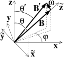
Figure 2: The laboratory $(x,y,z)$ and rotating $(\tilde{x},\tilde{y},\tilde{z})$ frames.

Berry phase for an isolated spin. We evaluate the BP for an isolated spin-half Berry (1984) using a rotating frame (RF)Berry87 , the one we choose (see Fig. 2) has its $\tilde{z}$-axis along the field ${\bf{B}}(t)$ and $\bm{e}_{\tilde{y}}\perp\bm{e}_{z}$ (then $\bm{e}_{\tilde{x}}(t_{\rm P})=\bm{e}_{\tilde{x}}(0)$). In this frame the magnetic field is ${\bf{B}}^{\prime}={\bf{B}}+{\bm{\omega}}$, where the angular velocity of the RF is

$${\bm{\omega}}=\dot{\theta}\,\bm{e}_{\tilde{y}}+\dot{\varphi}\,\bm{e}_{z}\ .$$ (1)

Transforming to the RF gives the Hamiltonian, $\tilde{H}=UH_{\rm spin}U^{-1}+i\dot{U}U^{-1}=-{\textstyle\frac{1}{2}}(\tilde{\bf{B}}+\tilde{\bm{\omega}})\hat{\mbox{\boldmath${\sigma}$}}$, where the transformation $U=\exp(i\theta\hat{\sigma}_{y}/2)\,\exp(i\varphi\hat{\sigma}_{z}/2)$ (with $B$, $\theta$, $\varphi$ being spherical coordinates of ${\bf{B}}(t)$)footnote:Pauli-matrices ; $\tilde{\bf{B}}=(0,0,B)$ and $\tilde{\bm{\omega}}=(\omega_{\tilde{x}},\omega_{\tilde{y}},\omega_{\tilde{z}})=(-\sin\theta\,\dot{\varphi},\dot{\theta},\cos\theta\,\dot{\varphi})$ are coordinates in the RF. The evolution in the RF is a rotation of the spin about the $\tilde{z}$-axis by the angle $\oint dt|{\bf{B}}^{\prime}(t)|$. To lowest order in $\omega$ the accumulated phase is $\int dt(B(t)+\omega_{\tilde{z}})$ footnote:RF . Subtracting the dynamical phase, we find the BP;

$$\Phi_{\rm BP}=\int dt\,\omega_{\tilde{z}}(t)\ =\oint d\varphi\,\cos\theta=\oint\!d{\bf{B}}\,{\bf{a}}({\bf{B}})\,.$$ (2)

In the chosen frame (gauge) the ‘vector potential’ ${\bf{a}}$ has only one non-zero spherical component $a_{\varphi}=1/(B\tan\theta)$. Stokes’ theorem is used to writing eq (2) as

$$\Phi_{\rm BP}=\int{d{\bf{S}}}\,{\bf{b}}({\bf{B}}),\ \ {\bf{b}}({\bf{B}})\equiv{\bf\nabla}_{\bf{B}}\times{\bf{a}}({\bf{B}})\,,$$ (3)

where ${\bf\nabla}_{{\bf{B}}}$ denotes derivatives w.r.t. the components of ${\bf{B}}$, and the field ${\bf{b}}({\bf{B}})$ is that of a charge-one monopole, $b_{B}=1/B^{2}$.

Environmental contribution to BP. Adding a noisy environment-induced field $\hat{{\bf{X}}}(t)\equiv\hat{X}(t)\bm{e}_{z}$, the Hamiltonian reads (in the lab frame)footnote:units

$$\hat{H}=-{\textstyle\frac{1}{2}}{\bf B}(t)\hat{\mbox{\boldmath${\sigma}$}}-{\textstyle\frac{1}{2}}\hat{X}\hat{\sigma}_{z}+\hat{H}_{\rm env}(\hat{X})\ .$$ (4)

This Hamiltonian models a situation in which the spin-environment coupling is strongly anisotropic. This is often true for solid-state qubits, where various ‘spin’ components couple to entirely different environmental degrees of freedom Nakamura et al. (1999); Vion et al. (2002); Chiorescu et al. (2002). Our analysis is easily generalized for multi-directional couplingfootnote4 . Below we express our results in terms of the statistical properties (correlators) of the environment’s noise, $\hat{X}(t)$. We consider any environment which gives rise to Markovian evolution, i.e. $\langle\hat{X}(t)\hat{X}(0)\rangle$ decays on a timescale $\tau\ll t_{\rm P},T_{\rm diss}\equiv{\rm min}(T_{1},T_{2},\delta B_{\rm Lamb}^{-1})$ however we do not assume $\tau\ll B^{-1}$. We further consider weak dissipation such that $BT_{\rm diss}\gg 1$. In the RF the Hamiltonian reads:

$$\tilde{H}=-{\textstyle\frac{1}{2}}B(t)\hat{\sigma}_{z}-\,{\textstyle\frac{1}{2}}\tilde{\bm{\omega}}(t)\hat{{\bm{\sigma}}}-{\textstyle\frac{1}{2}}\hat{X}(\cos\theta\hat{\sigma}_{z}-\sin\theta\hat{\sigma}_{x})+\hat{H}_{\rm env}\,.$$ (5)

We analyze this system in the eigen-basis of $B(t)\hat{\sigma}_{z}+\tilde{\bm{\omega}}(t)\hat{{\bm{\sigma}}}$, with the total field $B^{\prime}(t)\approx B(t)+\omega_{\tilde{z}}$ and the new angle $\theta^{\prime}$ as defined in Fig. 2.

The small terms $\propto\omega,\langle\hat{X}^{2}\rangle$ induce corrections to the evolution. As discussed above, the correction $\propto\omega$ to the rate of phase accumulation yields the BP, while the correction $\propto\langle\hat{X}^{2}\rangle$ gives $T_{1}^{-1},T_{2}^{-1},\delta B_{\rm Lamb}$. Here we evaluate the environment-induced BP $\propto\langle\hat{X}^{2}\rangle\omega$. To this end, we reduced the problem with a time-dependent field to a problem with a stationary field (to leading order footnote:RF ) by going to the RF and then use the standard formalism for evaluation of dissipative effects.

Consider the kinetic equation for the reduced density matrix of the spin $\rho$. Iteration of the Liouville equation Bloch (1957); Redfield (1957); textbooks ; Schoeller and Schön (1994); MSS-review leads to a Dyson-type master equation:

$$\dot{\rho}_{ij}(t)=\frac{{\rm i}}{2}\left[B^{\prime}\sigma_{z},\rho(t)\right]_{ij}\!+\!\int_{0}^{t}\!\!\!dt_{1}\Sigma_{ij,i^{\prime}j^{\prime}}(t,t_{1})\rho_{i^{\prime}j^{\prime}}(t_{1})\ .$$ (6)

The ‘self-energy’ $\Sigma(t,t_{1})$ can be evaluated perturbatively in $\hat{X}$; diagrammatically it is the sum of irreducible diagrams Schoeller and Schön (1994); MSS-review . For short-correlated noise $\tau\ll T_{\rm diss}$, one can make a Bloch-Redfield approximation Bloch (1957); Redfield (1957) giving Markovian evolution. We need only consider the off-diagonal density matrix element, $\rho_{12}(t)$, as it contains all phases (and dephasing) . After a secular approximation (for $\Gamma\ll B^{\prime}$) Landau and Lifshitz (1974), it is given by footnote-limit-on-integral

$$\dot{\rho}_{12}(t)=\left[{\rm i}B^{\prime}(t)+\Gamma(t)\right]\,\rho_{12}(t)\,,$$ (7)

$$\Gamma(t)\equiv\int\nolimits_{-\infty}^{t}dt_{1}\;\Sigma_{12,12}(t,t_{1})\;\exp\left(-{\rm i}\int\nolimits_{t_{1}}^{t}B^{\prime}(\tau)d\tau\right)\,.$$ (8)

We follow Bloch (1957); Redfield (1957); Schoeller and Schön (1994); MSS-review evaluating $\Sigma_{12,12}$ to lowest order ($2^{\rm nd}$-order) in $\hat{X}$. This “golden-rule” calculation yields

$$\Gamma(t) = -\int\nolimits_{-\infty}^{t}dt_{1}S(t-t_{1})\Big{[}\cos\theta^{\prime}(t)\cos\theta^{\prime}(t_{1})$$ (9)

$$+{\textstyle\frac{1}{2}}\sin\theta^{\prime}(t)\sin\theta^{\prime}(t_{1})\exp\left({-{\rm i}{\textstyle\int_{t_{1}}^{t}}B^{\prime}(\tau)d\tau}\right)\Big{]}\ ,\qquad$$

where $S(t-t_{1})\equiv(1/2)\left\{\langle\hat{X}(t)\hat{X}(t_{1})\rangle+\langle\hat{X}(t_{1})\hat{X}(t)\rangle\right\}$ is the symmetrized environment correlator Whitney et al. (2004). If we neglect all order-$\omega$ effects, we obtain

$$\Gamma_{0}(t)=-\frac{{\rm i}}{2}\int\!\frac{d\Omega}{2\pi}\,S(\Omega)\left[\frac{\sin^{2}\theta(t)}{\Omega-B+{\rm i}0^{+}}+\frac{2\cos^{2}\theta(t)}{\Omega+{\rm i}0^{+}}\right]\quad$$ (10)

where the integral is along the real axis and the function $S(\Omega)$ is the Fourier transform of $S(\tau)$, it is real and even. The real part of $\Gamma_{0}$ is the dephasing rate, which is given by the residue of the poles at $\Omega=0,B$. The imaginary part of $\Gamma_{0}$ is the Lamb shift, coming from the principal value of the integral (only the $\sin^{2}\theta$ term contributes).

Now we take into account the order-$\omega$ term in ${\bf{B}}^{\prime}(t)$ and the time-dependence of ${\bf{B}}^{\prime}(t)$; variations of the angle between ${\bf{B}}$ and ${\bf{X}}$ and of $B=|{\bf{B}}|$ [i.e. $\theta(t_{1})\neq\theta(t)$ and $B(\tau)\neq B(t)$ in (9)]. To lowest order in $\omega$ the modification of the rate (10) are:

$$\delta_{\varphi}\Gamma(t) = {\rm i}\dot{\varphi}\,\sin^{2}\theta(t)\cos\theta(t)\times F(B)\,,$$ (11)

$$\delta_{\theta}\Gamma(t) = {\rm i}\dot{\theta}\,\sin\theta(t)\cos\theta(t)\times G(B)\,,$$

$$\delta_{B}\Gamma(t) = {\rm i}\dot{B}\,\sin^{2}\theta(t)\times{\textstyle\frac{1}{2}}G^{\prime}(B)\,,$$

the dot indicates $({\rm d}/{\rm d}t)$, the prime indicates $({\rm d}/{\rm d}B)$, and

$$F(B) \equiv {\rm i}\frac{S(0)}{B}-\frac{1}{2}\int\frac{d\Omega}{2\pi}\,\frac{S(\Omega)\left(3B-2\Omega\right)}{B(\Omega-B+{\rm i}0^{+})^{2}}\,,$$ (12)

$$G(B) \equiv \frac{{\rm i}}{2}\int\frac{d\Omega}{2\pi}\left[\frac{S(\Omega)}{(\Omega-B+i0^{+})^{2}}-\frac{2S(\Omega)}{(\Omega+{\rm i}0^{+})^{2}}\right]\,.$$

From Eq. (7) one sees that these ${\cal O}[\omega]$-terms in $\Gamma(t)$ generate ${\cal O}[\omega^{0}]$-terms in the total phase acquired by $\rho_{12}$: $\delta\Phi_{\rm BP}=\int[F(B)\sin^{2}\theta\cos\theta\,d\varphi+G(B)\sin\theta\cos\theta\,d\theta$ $+\frac{1}{2}G^{\prime}(B)\sin^{2}\theta\,dB]$. This is geometric, and corresponds to $\delta\Phi_{\rm BP}=\int{\rm d}{\bf{B}}\,\delta{\bf{a}}({\bf{B}})$ (cf. eq. (2)) with the complex ‘vector potential’

$$\delta a_{\varphi}=B^{-1}F(B)\sin\theta\cos\theta\,,$$ (13)

$$\delta a_{\theta}=B^{-1}G(B)\sin\theta\cos\theta\,,\quad\delta a_{B}={\textstyle\frac{1}{2}}G^{\prime}(B)\sin^{2}\theta\,,$$

For open-paths of ${\bf B}(t)$ this is our main result, the imaginary part of this field (which gives geometric dephasing) is gauge-independent, while the real part is not. For closed paths of ${\bf B}(t)$ we use Stokes’ theorem to write $\delta\Phi_{\rm BP}=\int{d{\bf{S}}}\,\delta{\bf{b}}({\bf{B}})$ (cf. eq. (3)), finding that $\delta{\bf{b}}({\bf{B}})\equiv{\bf\nabla}_{{\bf{B}}}\times{\delta{\bf{a}}}$ has two non-zero components;

$$\delta b_{B} = B^{-2}F(B)(3\cos^{2}\theta-1)\,,$$ (14)

$$\delta b_{\theta} = -B^{-1}F^{\prime}(B)\sin\theta\cos\theta\,.$$ (15)

Thus it is independent of $\delta a_{\theta}$ and $\delta a_{B}$, their only role (for closed paths of ${\bf{B}}(t)$) is to form a ‘pure gauge’; this is related to a symmetry discussed below. The angular dependence of $\delta{\bf{b}}$ resembles that of a quadrupole. For slow environment modes ($\Omega\ll B$), ${\rm Re}[F(B)]\propto B^{-2}$ and hence $\delta{\bf{b}}({\bf{B}})$ is a quadrupole field. For other environment modes, $\delta{\bf{b}}({\bf{B}})$ has non-zero curl and zero divergence. Thus it is not a sum multipoles, it is the field generated by a pseudo-current, ${\bf{j}}({\bf{B}})\equiv{\bf\nabla}_{{\bf{B}}}\times{\bf{b}}({\bf{B}})$, with one non-zero component

$$j_{\varphi}(B)=B^{-3}\big{(}6F(B)-B^{2}F^{\prime\prime}(B)\big{)}\sin\theta\cos\theta\,.$$ (16)

Since we can ignore $\delta a_{\theta}$ and $\delta a_{B}$ for closed paths, eq. (13) leads to the following pretty result: the total (complex) BP for a closed path is

$$\Phi_{\rm BP}=\oint{\rm d}\varphi\ \frac{{\rm d}}{{\rm d}{B_{z}}}(B+\delta B_{\rm Lamb}+{\rm i}T_{2}^{-1})\ .$$ (17)

This result can be understood as follows. For a time-independent ${\bf{B}}$ the acquired phase is $\int dt\,{\cal E}$, where ${\cal E}$ is the term in parentheses in Eq. (17). When ${\bf{B}}$ is time-dependent, ${\bf{B}}\rightarrow{\bf{B}}+{\bm{\omega}}$ in the RF changing the phase by $\int dt\,{\bm{\omega}}{\bf\nabla_{B}}{\cal E}$; with Eq. (1) this gives Eq. (17).

Symmetry considerations. We now show that the vanishing of $b_{\varphi}$ follows from the symmetries of the problem. Firstly, under time-reversal ${\bf{B}}(t),{\bf{X}}(t)\to-{\bf{B}}(-t),-{\bf{X}}(-t)$ the BP between the excited and ground states is invariant, while in eq. (3) $d{\bf{S}}\to-d{\bf{S}}$. This implies that ${\bf b}(-{\bf{B}},-X)=-{\bf{b}}({\bf{B}},X)$. Secondly, if we instead rotate all spins and fields by angle $\pi$ about the axis $\hat{\varphi}$ perpendicular to both ${\bf{B}}$ and $X$ (e.g. ${\bf{B}}\to-{\bf{B}}$), the field ${\bf{b}}$ would also rotate. Thus, ${\bf{b}}(-{\bf{B}},-X)=R^{\pi}_{\varphi}{\bf{b}}({\bf{B}},X)$. To satisfy both equalities, $b_{\varphi}\equiv 0$.

For isotropic coupling, the Hamiltonian’s rotational symmetry guarantees that $b_{\varphi}=b_{\theta}=0$. The monopole (cf. eq. (3)) is quantized so $\delta b_{B}=0$; hence $\delta\Phi_{\rm BP}=0$ to all orders in the coupling to the environment.

Contribution of the slow modes ($\Omega\ll B$). Here $F(B)\propto B^{-2}$, so $\delta{\bf b}$ is a quadrupole field. This effect of (for instance, classical) slow modes can be understood by noting that $({\bf{B}}(t)+{\bf{X}}(t))$ varies adiabatically, hence

$$\Phi_{\rm BP}=\oint d({\bf{B}}+{\bf{X}}){{\bf{a}}_{\rm m}}({\bf{B}}+{\bf{X}})=\oint d{\bf{B}}{{\bf{a}}_{\rm m}}({\bf{B}}+{\bf{X}})\,,$$ (18)

where ${{\bf{a}}_{\rm m}}$ is the field of a charge-one monopole at the origin. We disregard boundary corrections due to ${\bf{X}}(t_{\rm P})\neq{\bf{X}}(0)$ and drop the term $\oint d{\bf{X}}\,{{\bf{a}}_{\rm m}}({\bf{B}}+{\bf{X}})$ footnote5 . The remaining term is the field of a monopole at the point $-{\bf{X}}$. In the multipole expansion, ${{\bf{a}}_{\rm m}}({\bf{B}}+{\bf{X}})={{\bf{a}}_{\rm m}}({\bf{B}})+X_{\alpha}\nabla_{\alpha}{{\bf{a}}_{\rm m}}({\bf{B}})+{\textstyle\frac{1}{2}}X_{\alpha}X_{\beta}\nabla_{\alpha}\nabla_{\beta}{{\bf{a}}_{\rm m}}({\bf{B}})+\cdots$. The first term produces the unperturbed BP, the second (dipole) term vanishes after averaging over the fluctuations DeChiaraPalma . Thus the quadrupole term gives the leading environment-induced modification of the BP. For noise along the $z$-axis this term reads $D_{\alpha\beta}\nabla_{\alpha}\nabla_{\beta}{{\bf{a}}_{\rm m}}/6$, with the quadrupole moment $D_{\alpha\beta}=\langle X^{2}\rangle\mathop{\rm diag}(-1,-1,2)$.

Concerning experiments. Our results imply that the traversal of the same loop ${\bf{B}}(t)$ in opposite directions would yield, apart from different BP’s, different dephasing. We further note that a noise spectrum suppressed at $\Omega=0$, $B$ will increase $T_{2}$ while having little effect on $\delta\Phi_{\rm BP}$, thus aiding the observation of $\delta\Phi_{\rm BP}$.

This work is part of CFN (DFG), supported in part by the Minerva (DFG) Foundation, the EC-RTN Spintronics, and ISF of IAS. RW, YM and YG were supported by the EPSRC, the Dynasty Foundation and the AvH Foundation (Max-Planck award) respectively. The Transnational Access prog. supported the WIS visit of YM,AS.

References

- Berry (1984) M. V. Berry, Proc. R. Soc. Lond. 392, 45 (1984).
- Whitney and Gefen (2003) R.S. Whitney and Y. Gefen, Phys. Rev. Lett. 90, 190402 (2003).
- Nakamura et al. (1999) Y. Nakamura, Yu. A. Pashkin, and J. S. Tsai, Nature 398, 786 (1999).
- Vion et al. (2002) D. Vion, A. Aassime, A. Cottet, P. Joyez, H. Pothier, C. Urbina, D. Esteve, and M. H. Devoret, Science 296, 886 (2002).
- Chiorescu et al. (2002) I. Chiorescu, Y. Nakamura, C. J. P. M. Harmans, and J. E. Mooij, Science 299, 1869 (2002).
- Falci et al. (2000) G. Falci, R. Fazio, G. H. Palma, J. Siewert, and V. Vedral, Nature 407, 355 (2000).
- (7) All energies and magnetic fields are in units of inverse time ().
- Garrison and Wright (1988) J. C. Garrison and E. M. Wright, Phys. Lett. A 128, 177 (1988).
- see e.g. D. Ellinas et al. (1989) see e.g. D. Ellinas, S. M. Barnett, and M. A. Dupertuis, Phys. Rev. A 39, 3228 (1989), D. Gamliel, J. H. Freed, Phys. Rev. A 39, 3238 (1989); A. Carollo, I. Fuentes-Guridi, M.F. Santos, and V. Vedral, Phys. Rev. Lett. 90, 160402 (2003).
- Gaitan (1998) F. Gaitan, Phys. Rev. A 58, 1665 (1998), J.E. Avron, A. Elgart, Phys. Rev. A 58, 4300 (1998).
- (11) G. De Chiara and G. M. Palma, Phys. Rev. Lett. 91, 090404 (2003) consider only the dipole slow-noise term and thus do not find , cf. below our eq. (18).
- (12) Here we ignore the boundary terms, ; cf. Whitney and Gefen (2003).
- (13) If traverses a loop times in a time , the leading non-adiabatic correction , while . We can separate the two by varying (keeping ) or . Alternatively the environment’s spectrum may make non-adiabatic effects , because comes from the whole spectrum while is dominated by frequencies (see below eq. (10)).
- Wilczek and Zee (1984) F. Wilczek and A. Zee, Phys. Rev. Lett. 52, 2111 (1984).
- (15) M.V. Berry, Proc. R. Soc. Lond. A, 414, 31 (1987).
- (16) To avoid confusion we define as the same Pauli matrices, e. g. , in all frames.
- (17) Typically in the RF is non-stationary and is not quite parallel to the -axis. This only gives non-adiabatic corrections, ; cf. Berry87 .
- (18) For multi-directional coupling is the sum of the s calculated separately for each coupling axis to . We find for isotropic coupling.
- (19) see e.g. U. Weiss, Quantum dissipative systems (World Scientific, Singapore, 1999). C. Cohen-Tannoudji, J. Dupont-Roc and G. Grynberg, Atom-photon interactions (Wiley, New York, 1992).
- Bloch (1957) F. Bloch, Phys. Rev. 105, 1206 (1957).
- Redfield (1957) A. G. Redfield, IBM J. Res. Dev. 1, 19 (1957).
- Schoeller and Schön (1994) H. Schoeller and G. Schön, Phys. Rev. B 50, 18436 (1994).
- (23) For an introduction see Yu. Makhlin, G. Schön, and A. Shnirman in New Directions in Mesoscopic Physics Edited by V.F. Gantmakher, R. Fazio, and Y. Imry (Kluwer Academic, Dordrecht, 2003) p. 197.
- Landau and Lifshitz (1974) L. D. Landau and E. M. Lifshitz, Quantum Mechanics (Pergamon, Oxford, 1974), chap. VI.
- (25) The above integral is dominated by close to thus we can take the lower bound of integration to with little effect (except at small where it causes a small “preparation” correction).
- Whitney et al. (2004) R. S. Whitney, Yu. Makhlin, A. Shnirman, and Y. Gefen, in cond-mat/0401376 (2004).
- (27) Since for in the chosen gauge ; this also holds for general as long as and have equal weights since their contributions cancel.