The in-plane electrodynamics of the superconductivity in Bi₂Sr₂CaCu₂O_8+δ: energy scales and spectral weight distribution

Abstract

The in-plane infrared and visible (3 meV–3 eV) reflectivity of Bi₂Sr₂CaCu₂O_8+δ (Bi-2212) thin films is measured between 300 K and 10 K for different doping levels with unprecedented accuracy. The optical conductivity is derived through an accurate fitting procedure. We study the transfer of spectral weight from finite energy into the superfluid as the system becomes superconducting. In the over-doped regime, the superfluid develops at the expense of states lying below 60 meV, a conventional energy of the order of a few times the superconducting gap. In the underdoped regime, spectral weight is removed from up to 2 eV, far beyond any conventional scale. The intraband spectral weight change between the normal and superconducting state, if analyzed in terms of a change of kinetic energy is $\sim 1$ meV. Compared to the condensation energy, this figure addresses the issue of a kinetic energy driven mechanism.

I INTRODUCTION

Cuprate superconductors, where the electronic correlations are important, deviate in many fundamental aspects from conventional superconductors. The electronic structure of these materials presents a strong momentum dependence, as demonstrated from, e.g., angle-resolved photoemission spectroscopy (ARPES) experiments.Olson-FS ; FSinBSCCO ; Campuzano-FSinYBCO ; Dessau-FS ; Campuzano-NoBilayer ; Campuzano-FSinBSCO This plays a definite role in the optical and transport phenomena of these high-$T_{c}$ materials,BasovVDM ; Orenstein-NodalTau and has noticeable consequences in the pseudogap regime Andres-PRL-PSG (for an experimental review of the pseudogap, see the reference TimuskStattPG ).

In the superconducting state, the binding of quasi-particles (QP) into Cooper pairs and the concomitant onset of phase coherence between the pair states are well understood in the case of conventional metals. The pairing mechanism and the formation of a coherent state remains a central problem in high-$T_{c}$ superconductivity. Various unanswered and possibly contradictory issues are being debated concerning the nature of the pseudogap state (PGS) and its temperature onset.Puchkov-PropOpt

In this paper, we focus on a quantitative analysis in the superconducting state (SCS). More precisely, we investigate the spectral weight $W$, i.e. the area under the real part of the optical conductivity, defined as:

$$W=\int_{0^{+}}^{\omega_{c}}\sigma_{1}(\omega,T)d\omega,$$ (1)

where $\sigma_{1}(\omega,T)$ is the frequency ($\omega$) and temperature ($T$) dependent conductivity, and $\omega_{c}$ is a cut-off frequency. The optical conductivity being related to the absorption, the spectral weight calculated up to $\omega_{c}$ reflects the number of states available for an optical transition up to this energy. It has been known for a long time that there is a noticeable loss of spectral weight in the optical conductivity when high $T_{c}$ materials enter the SCS. One key issue is the energy scale over which this loss of spectral weight occurs. It is indeed related to the excitations responsible for pairing. This loss of spectral weight occurs because as superconductivity sets in, single QP states are suppressed and the associated weight is transferred into the zero frequency peak associated with the superfluid condensate.

More precisely, the Ferrell-Glover-Tinkham (FGT) sum rule FGT-1 ; FGT-2 requires that the spectral weight $\Delta W$ lost when decreasing the temperature from the normal state into the superconducting state, must be retrieved in the spectral weight $W_{s}$ of the $\delta(\omega)$ function centered at zero frequency. The sum rule is exact if integrating up to infinity, and results merely from charge conservation. Actually, the sum rule is satisfied ($\Delta W\simeq W_{s}$) provided the integration is performed up to a large enough value $\hbar\Omega_{M}$. In conventional superconductors, $\hbar\Omega_{M}$ is typically $16k_{B}T_{c}$, or about $4\Delta$ ($\Delta$ is the superconducting gap).FGT-1 ; FGT-2 $\hbar\Omega_{M}$ is considered to be a characteristic energy of the boson spectrum responsible for the pairing mechanism. Would cuprates display this conventional behavior, then taking a typical maximum gap magnitude (in a d-wave superconductor) $\Delta_{M}$ of 25 meV yields $\hbar\Omega_{M}\sim 0.1$ eV.GapHTc-1 ; GapHTc-2 Indeed, from conventional BCS theory, including strong electron-phonon coupling, the amount of violation of the FGT sum rule is of the order of $(\Delta/\omega)^{2}$ for $\omega\gg 2\Delta$, hence negligible.Maksimov-SumRule

An apparent violation of the sum rule, i.e. $\Delta W<W_{s}$ when integrating up to 0.1 eV was observed from interlayer conductivity data: exhausting the sum rule could then require an anomalously large energy scale, which was suggested to be related to a change of interlayer kinetic energy when the superfluid builds up.Basov ; KatzBasov ; BasovVDM Although early measurements yielded conventional in-plane energy scales Basov , the decrease of the in-plane kinetic energy, suggested long ago as a possible pairing mechanism in the framework of the hole undressing scenario,Hirsch1-1 ; Hirsch1-2 was given renewed interest.Hirsch3-1 ; Hirsch3-2 ; Hirsch2 Indeed, later ellipsometric measurements and IR reflectivity experimentsRubhausen-100Delta ; vdmScience ; Boris showed that in-plane spectral weight was lost up to the visible range. The key issue which has to be addressed experimentally is whether this spectral weight is transferred into the condensate.Andres-EPL

The data presented in this paper report the investigation of the FGT sum rule in three carefully selected thin films from the Bi-2212 family, probing three typical locations in the phase diagram: the underdoped (UND), the optimally doped (OPT) and the overdoped (OVR) regime. A detailed study allows to work out with well controlled error bars the FGT sum rule and the spectral weight changes. We find that within these error bars, retrieving the condensate spectral weight in the OVR and OPT samples requires integrating up to an energy of the order of 0.1 eV (800 cm^-1), i.e. a conventional energy scale. In the UND sample, about 20% of the FGT sum rule is still missing at 1 eV, and the integration must be performed up to at least 16000 ${\rm cm}^{-1}$ (2 eV), an energy scale much larger than typical boson energies in a solid, and $\sim 100$ times larger than the maximum gap. We derive the associated change of the in-plane kinetic energy, which turns out to agree with some theoretical calculations.Hirsch3-1 ; Hirsch3-2 ; NormanPepin-QPFormation This paper supplements our previous report on the FGT sum rule,Andres-EPL by developing in detail the investigation on the spectral weight distribution in the superconducting state, and by presenting the details of the analysis of the thin-film reflectivity and of the uncertainties.

The paper is divided as follows: after a presentation of the experimental results, we will perform the analysis of the data in terms of the partial spectral weight and the FGT sum rule as a function of the cut-off frequency. We will give an interpretation of the results in terms of a change of the in-plane kinetic energy. In the appendix, we describe the sample fabrication, characterization and selection, and the experimental set-up. Then, we discuss the procedure to derive the optical functions from the reflectivity of a film deposited onto a substrate, giving a detailed account of the experimental uncertainties arising from this procedure, and explaining how we incorporated the uncertainties associated with the low temperature extrapolation of the normal-state spectral weight (which is required to compute correctly the FGT sum rule) into the total error bars.

II EXPERIMENTAL RESULTS

II.1 Samples and measurements

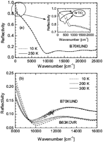
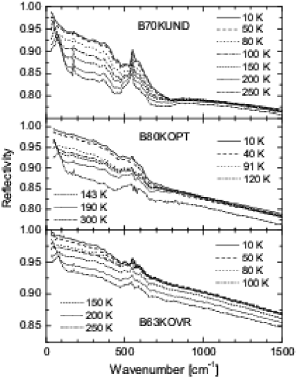
Figure 1: (a) Reflectivity of the B70KUND sample in the whole experimental range, at high (250 K) and low (10 K) temperatures. The inset shows the variation of the reflectivity in the far-infrared, and the phonon peaks from the substrate. (b) Temperature changes of reflectivity in the visible range for the B70KUND and B63KOVR samples. Right panels: reflectivity of the three samples, for a restricted set of temperatures, up to 1500 cm^-1.

The thin films studied in this work were epitaxially grown by r.f. magnetron sputtering on (100) SrTiO₃ substrates heated at temperatures $\gtrsim 700^{\circ}$C.Li-Films ; Zorica-Films X-ray analyses confirmed that the films are single phase, with the c-axis perpendicular to the substrate, and a cation ratio (in particular a Bi$/$Sr ratio) corresponding to the stoichiometric one.Zorica-Thesis Their maximum critical temperature (defined at zero resistance) obtained in these conditions is $\sim 84$ K. The $\mathbf{a}$ and $\mathbf{b}$ axes show a single orientation (45^∘ with respect to the substrate axes), with possible exchanges between $\mathbf{a}$ and $\mathbf{b}$ from one grain to another. The directions -Cu-O-Cu- are parallel to the (100) and (010) axes of the substrate. Films prepared by the above procedure are usually in a nearly optimally doped state. The various doping levels (UND and OVR) were obtained by post-annealing the films in a controlled atmosphere.Zorica-Films In total, thirteen samples of Bi-2212 thin films were investigated. All the films were first characterized by electrical resistance measurements, and a first estimate of their thicknesses was obtained by Rutherford Back-Scattering (RBS) on samples prepared under exactly the same conditions as the ones used in this work, on MgO substrates. Absolute resistivities were not measured, as this would have required a lithographic etching of the samples, which is incompatible with the optical measurements. As a next step, their optical homogeneity in the mid-infrared was characterized by infrared microscopy ($\mu$IR), as will be described in the appendix. The surface quality in the visible was characterized by optical microscopy.

Another Bi-2212 film on (100) LaAlO₃ single crystal substrate, prepared by a high-pressure dc sputtering technique, was also studied. Prieto In this case, pure oxygen at a 3.5 mbar pressure was used as sputtering gas, with a 880^∘C deposition temperature. Typical deposition rates being 1000 Å/h, the thickness of Bi-2212 films lies around 4000 Å. Films were post-annealed for 45 min at 0.01 mbar oxygen pressure, yielding films with an optimal oxygen content (maximum critical temperature $T_{c}$=90 K). Such fabricated films are single phase and c-axis oriented, as confirmed by different techniques. In $\theta-2\theta$ scan X-ray measurements, only (001) peaks were observed. The spread of the distribution of c-axis oriented grains tilted away from the surface was obtained from the rocking curves. Such rocking curves around the (001̆0) diffraction peak display a width at half-maximum $0.2-0.3^{\circ}$, indicating good crystalline quality of the samples. RBS combined with channeling measurements allowed to verify the composition and epitaxial quality of the layers. A mean roughness of around 4.5 nm in the surface of the films was found by atomic force microscopy (AFM). Because of their large thickness, the substrate contribution in such samples is almost negligible, providing us with a valuable test of the comparison between Kramers-Kronig data processing and our customized fitting procedure, as explained below. Finally a similar YBa₂Cu₃O₇ (YBCO) film at optimal doping, deposited onto LaAlO₃ was also studied for comparison (see appendix).

The full infrared-visible reflectivities, taken at typically 15 temperatures between 10 K and 300 K and at quasi-normal incidence ($\sim 8^{\circ}$), were measured for all the films in the spectral range $[30-7000]$ cm^-1 with a Bruker IFS 66v Fourier Transform spectrometer, supplemented with standard grating spectroscopy in the range $[4000-28000]$ cm^-1 (Cary-5).

To determine the absolute value of the reflectivity, we used as unity reflectivity references a gold mirror in the $30-7000$ cm^-1 spectral range, and a silver mirror in the remaining spectral range. To ensure accuracy in this absolute measurement, the sample holder was designed to allow to commute between the reference and the sample, placing one or the other at the same place, within an angular accuracy better than $10^{-3}$ rad, on the optical path, independently of the optical (light-entrance windows) or thermal (temperature) set-up of the cryostat. The latter is a home-built helium-flow cryostat, with the sample holder immersed in the helium flow, so that both sample and reference mirror are cooled simultaneously. The temperature in our set-up can be stabilized within 0.2 K. A circular aperture placed in front of the sample/reference position guarantees that the same flux is irradiating the sample and the reference. The temperature of the sample/reference block is measured independently of that of the helium flow. Once thermal equilibrium has been achieved in the entire cryogenic set-up, consecutive measurements of the sample and reference spectra can be done, under exactly the same conditions. Our accuracy in the determination of the absolute reflectivity is 1%.

In order to extract the optical functions from our raw measurements, we need to know the film thicknesses (as explained below). After the infrared measurements, the film thicknesses were directly determined by RBS for the OPT and OVR samples, yielding 395 nm and 270 nm respectively (The uncertainty in the thickness given by RBS on films grown on SrTiO₃ is 300 Å). A lower bound for the UND sample was estimated by RBS in a sample grown on MgO simultaneously to ours, yielding 220 nm. (The UND sample itself was destroyed in an unsuccessful attempt to measure its thickness by transmission electron microscopy).

It is known that temperature changes of the optical response of cuprates in the mid-infrared and the visible ranges are small, but, as discussed further, cannot be neglected.Maksimov Yet, as remarked by van der Marel and coworkers,vdMTrieste most studies rely on a single spectrum at one temperature in the visible. Moreover, few temperatures are measured, due to the lack of resolution when the temperature-induced reflectivity changes are small. Using thin films rather than single crystals allowed us to measure relative variations in the reflectivity within less than 0.2%, even in the visible range, due to their large surface (typically $6\times 6$ mm²). We were thus able to monitor the temperature evolution of the reflectivity spectra in the full available range (30-28000 cm^-1). This is obviously important if one is looking for a spectral weight transfer originating from (or going to) any part of the whole frequency range.

II.2 Raw data

Our films critical temperatures are 70 K (B70KUND), 80 K (B80KOPT) and 63 K (B63KOVD). Figure 1(a) shows two reflectivity curves (at $T=250$ K and $T=10$ K) of the B70KUND sample. This is an example of the typical spectra we have measured. The signal-to-noise ratio is unprecedented, and relative variations of the reflectivity of the order of 0.2% can be measured. In the far-infrared (see the inset), the three phonon peaks coming from the underlying substrate are clearly visible, specially at high temperatures (or low doping), when the system is less metallic. The lowest-energy peak is the soft mode of SrTiO₃. We experimentally determined the optical constants of the SrTiO₃ at each temperature, so as to take into account the changes in reflectivity due to changes in the substrate optical properties alone. This is important when extracting the intrinsic optical constants of the Bi-2212 (the procedure will be described below).

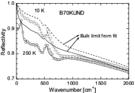
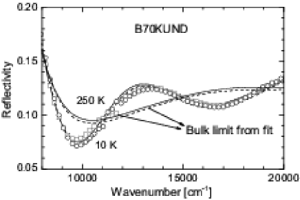
Figure 2: Measured reflectivity spectra of the B70KUND sample at 250 K and 10 K (open symbols) and fitted spectra (lines) at far-infrared (left panel) and visible (right panel) frequencies. The fits lie within $\pm 0.1$% of the raw data in the full spectral range (up to 25000 cm^-1). The bulk reflectivities obtained from the fits are also shown. Note that the contribution from the substrate to the raw data is effectively suppressed in the bulk reflectivities.

While the major temperature changes in the reflectivity occur at low frequency, where reflectivity increases with increasing doping or decreasing $T$, changes up to the visible range (up to $\sim 12000-14000$ cm^-1) are important as well. This is illustrated for the B70KUND and B63KOVR samples in Fig. 1(b). This figure shows indeed that, in the visible range, a decrease in doping has the same qualitative effect that increasing the temperature: in both cases, the reflectivity in the visible range increases. This effect disappears below temperatures close to $T_{c}$: there is no measurable change in the visible reflectivity below $\sim 100$ K. These opposite temperature behaviors of the infrared and visible reflectivities have been observed as well by temperature-modulated differential spectroscopy measurements.Holcomb ; Little The oscillations in the reflectivity in the visible range come from both interband transitions and interferences of the light bouncing back and forth inside the film. The period of these oscillations, and the shape of the reflectivity in the vicinity of the plasma edge, depend on the sample thickness.

The right panels of Fig. 1 show the reflectivities of the three samples, for a restricted set of temperatures, up to 1500 cm^-1. Note that, upon increasing doping, the reflectivity increases for a given temperature in this spectral range, as a consequence of the material becoming more metallic.

II.3 Extraction of the optical functions

The contributions of the substrate to the measured reflectivities preclude the Kramers-Kronig (KK) analysis on thin films. In order to extract the optical functions intrinsic to Bi-2212, we simulated its dielectric function at each temperature and doping levels using Drude-Lorentz oscillators (thus warranting causality). In the superconducting state, where a superfluid exists, we used a London oscillator as well. The London oscillator is indeed necessary to simulate properly the change in slope in the reflectivity observed at low frequencies and low temperatures (Fig. 1, right panels). We then modelled the reflectance of the film on top of a substrate, using the optical constants of SrTiO₃ that, as already stated, were experimentally determined for each temperature. We found that the best description of our data was obtained by assuming an infinitely thick substrate (i.e., no backward reflection from the rear of the substrate; see the Appendix for details). Finally, we adjusted the attempt dielectric function of the Bi-2212 in order to fit accurately the raw reflectivity spectra. Examples of such fits, for the B70KUND sample, are shown in Fig. 2 at far-infrared (left panel) and visible (right panel) frequencies. Once the dielectric function is known, we can generate any other optical function, in particular the optical conductivity.

We have verified that, in average over the whole experimental range, a relative error $\Delta R/R$ in the fit yields a relative error magnified by at most a factor 10 in the real part of the optical conductivity, provided that $\Delta R/R\ll 1$. These relative errors spread over $2-3$ times the range where the deviation to the raw data occurs (see the Appendix, in particular Fig. 9, for details). The thicknesses of the films are also determined by the fit. Fits are accurate within less than 0.5% taking 241, 434 and 297 nm for the B70KUND, B80KOPT and B63KOVR samples respectively. These values differ by less than 10% from the RBS measurements. We checked that the associate error in the conductivity, within the experimentally measured range, is less than 10%. The fit yields a valuable extrapolation of the conductivity in the low-energy range ($\hbar\omega<30$ cm^-1, not available experimentally),Quijada which is important in the evaluation of the spectral weight. In this range, however, the relative error in the conductivity was calculated and reaches 20%.Andres-PRL-PSG

We have used the thick optimally doped film ($T_{c}$=90 K) as a further check of the validity of the fitting procedure. We have compared the conductivities extracted by the fitting procedure (after full characterization of the LaAlO₃ substrate) to the ones obtained by performing a Kramers-Kronig transform of the raw reflectivity data. The reason for this attempt is that the fits show a reconstructed bulk reflectivity for this sample differing within less than 1 % from the raw spectrum, in the whole spectral range. This turns out to have a dramatic impact on the conductivity below 100 cm^-1. However, above this frequency, the conductivities deduced from the fit and from KK transform lie within 20 % one from the other, with a systematic trend placing the KK result above the result from the fit. This observation is entirely compatible with all the estimates presented in the appendix. It shows moreover that the fitting is absolutely required for the low frequency analysis and the eventual spectral weight calculations: it is the low frequency range where the penetration length of the electromagnetic wave is large and therefore where the substrate effects are the most detrimental.

Figure 3 shows the conductivity spectra for the B70KUND, B80KOPT and B63KOVR samples, for the same temperatures and in the same spectral range as the reflectivity spectra of Fig. 1. Note that the conductivity values are larger for the overdoped sample, in agreement with a larger density of charge carriers. The low-frequency values of the conductivity are reasonable figures for Bi-2212: at 250 K, for example, our DC extrapolations give as resistivities $\rho_{ab}\approx 500$ $\mu\Omega$-cm for the underdoped sample, and $\rho_{ab}\approx 160$ $\mu\Omega$-cm for the overdoped one. Furthermore, as can be seen in Fig. 4, the temperature behavior of the DC extrapolations is in agreement with the resistance measurements. For the underdoped sample, the two data points within the resistive transition do not follow the trend of the measured resistance. Whatever the phenomenon causing the large resistive transition (a well documented feature in underdoped Bi-2212 films Eckstein-Raffy ) it is not taken into account in our analysis, which assumes an homogeneous material. In this respect, the London oscillator used for our fits was only “turned-on” at $T<T_{c}$ (defined by zero-resistance).

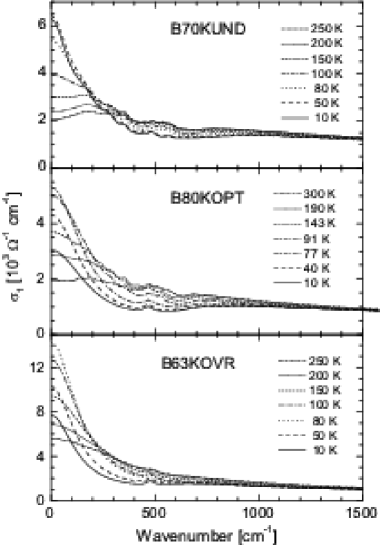
Figure 3: Selection of conductivity spectra for the B70KUND (upper), B80KOPT (middle) and B63KOVR (lower) samples. For the B70KUND sample, within the showed spectral range, the spectra at 50 K and 10 K are indistinguishable. The error bars in the conductivity spectra are $\Delta\sigma/\sigma\lesssim 10$% for $\hbar\omega>30$ cm^-1, and $\Delta\sigma/\sigma\sim 20$% for $\hbar\omega<30$ cm^-1.

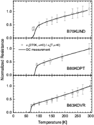
Figure 4: Measured resistance of the three selected samples (normalized to unity at high temperatures), and comparison with the DC extrapolation of the respective conductivities obtained from the reflectivity spectra.

In the normal state, the conductivity spectra of the three samples are qualitatively similar. The weak shoulder at $\sim 200$ cm^-1 visible in the UND sample down to 150 K has been observed in single crystals as well,Puchkov-PropOpt and remains unexplained so far. The low-frequency conductivity ($\hbar\omega\lesssim 200$ cm^-1) of the three samples increases when the temperature decreases (metallic behavior), while at higher frequencies, because of the conservation of the spectral weight, the conductivity decreases when the temperature drops. The conservation of the spectral weight in the normal state is retrieved upon integration up to $\sim 2$ eV. The implications of such observation on the electrodynamics of the normal state have already been analyzed.Andres-PRL-PSG

The superconducting transition is marked, for the overdoped and optimally-doped samples, by a decrease of the conductivity over the spectral range shown in Fig. 3. This effect becomes more pronounced as the temperature continues to drop, so that a clear loss of spectral weight, associated with the formation of the zero-frequency condensate, is observed in this spectral range. In contrast, the low-frequency ($\hbar\omega\lesssim 100$ cm^-1) conductivity of the underdoped sample does not decrease when temperature decreases below $T_{c}$, and a large Drude-like contribution persists in the superconducting state. Beyond this energy scale, the normal- and superconducting-state conductivities cross, and there is no clear loss of spectral weight within the spectral range shown in the figure. A deeper analysis is needed in this case, based on the FGT sum rule.

III ANALYSIS AND INTERPRETATION

III.1 In-plane FGT sum rule for Bi-2212

Be $T_{A}\geq T_{c}$, and $T_{B}<T_{c}$. From an experimental point of view, the FGT sum rule compares the change in spectral weight $\Delta W=W(T_{A})-W(T_{B})$ (Eq. 1) and the supefluid weight $W_{s}$.

Within the London approximation, at frequencies below $\Delta_{M}$, the slope of the real part of the dielectric function $\epsilon_{1}\left(\omega\right)$ plotted versus $1/\omega^{2}$ should be directly related (as was done in our previous report Andres-EPL ) to the superfluid spectral weight $W_{s}$ through the “London” frequency $\Omega_{L}=c/\lambda_{L}$, where $\lambda_{L}$ is the London penetration depth. However, for the underdoped sample, the presence of a large Drude-like contribution to the conductivity in the superconducting state yields, by this procedure, an overestimate of about $15-20$% on $\Omega_{L}^{2}$ (i.e., on the superfluid weight).MN-Private A simulation of this effect shows that, for this sample, the best estimate for the value of $\Omega_{L}$ is the input parameter of the fit, whose accuracy (within $0.1\%$) we have carefully re-worked out. For the optimally doped and overdoped samples there is no significant difference between the slope of the $\epsilon_{1}$ versus $\omega^{-2}$ plot and the superfluid input parameters of the fits, in accordance with a weaker contribution of the charge carriers to the superconducting low-frequency conductivity (Fig. 3, middle and lower panels).

In this way we find that, at 10 K, $\lambda_{L}=6250$ Å, 2900 Å and 2250 Å for the B70KUND, B80KOPT and B63KOVR samples respectively. The values for the overdoped and optimally doped samples are in fair agreement with those reported in the literature.Villard-Lambda There are no reliable data on the absolute value of the London penetration depth for underdoped samples.DiCastro-Lambda

Figure 5 shows the ratio $\Delta W/W_{s}$ for the three samples reported in this work. The changes in spectral weight are taken between 80 K–10 K, 91 K–10 K and 100 K–10 K for the OVR, OPT and UND samples respectively, so that the normal-state temperature lies slightly above the resistive transition regime. In the underdoped sample, we find that at energies as large as 1 eV (8000 cm^-1) $\Delta W/W_{s}\sim 0.8\pm 0.15$ (details about the evaluation of the error bars will be given below). It approaches 1 at $\sim 16000$ cm^-1. A Kramers-Kronig based analysis shows that, beyond this frequency range, the error in the determination of the conductivity (hence the spectral weight) rapidly increases. This is a consequence of the reflectivity for $\hbar\omega>25000$ cm^-1 not being available experimentally (see the Appendix for further details).

A large part ($\sim 20$ %) of the superfluid weight in the underdoped regime thus builds up at the expense of spectral weight coming from high energy regions of the optical spectrum ($\hbar\omega\geq 1$ eV). Because of our error bars, we cannot make a similar statement for the optimally doped and overdoped samples, where the sum rule may be exhausted at roughly $500-1000$ cm^-1. The FGT sum rule has been also worked out for the thick Bi-2212 sample using the conductivities deduced from the fit. We do find in this case as well that the sum rule is satisfied for a conventional energy scale (1000 cm^-1).

Our results for the optimally doped and overdoped samples thus do not contradict earlier similar work in YBCO and Tl₂Ba₂CuO_6+δ (Tl-2212).BasovVDM A recent work on underdoped YBCO shows that, in the spectral region where the temperature dependence of the spectra was measured (up to about $5000$ cm^-1), the FGT sum rule is not saturated.Homes-SumRules On the other hand, our results in the underdoped regime are in agreement with recent ellipsometric measurements in the visible range which shown that in-plane spectral weight is lost in the visible range.Rubhausen-100Delta ; vdmScience However, the latter results did not provide direct evidence that this spectral weight is indeed transferred into the condensate.

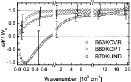
Figure 5: Ratio $\Delta W/W_{s}$ versus frequency showing the exhaustion of the FGT sum rule at conventional energies for the OVR (solid lines, right error bars) and OPT (dashed lines, middle error bars) samples. An unconventional ($\sim 16000~{}{\rm cm}^{-1}$ or 2 eV) energy scale is required for the UND sample (short-dashed lines, left error bars). Note that the frequency scale changes at $800$ and $8000$ cm^-1. The changes in spectral weight are taken between 80 K–10 K, 91 K–10 K and 100 K–10 K for the OVR, OPT and UND samples, respectively.

The remarkable behavior of the underdoped sample must be critically examined in light of the uncertainties that enter in the determination of the ratio $\Delta W/W_{s}$. The determination of $\Delta W$ assumes that $W(T_{A})$ is a fair estimate of the spectral weight obtained at $T_{B}<T_{c}$, defined as $W_{n}(T_{B})$, if the system could be driven normal at that temperature. While this assumption is correct in BCS superconductors, it may no longer be valid for high-$T_{c}$ superconductors.Chakravarty Hence, our taking the normal-state spectral weight $W(T_{A}\geq T_{c})$ instead of $W_{n}(T_{B})$ (unknown) may bias the sum rule.

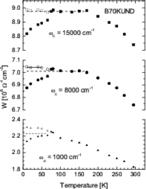
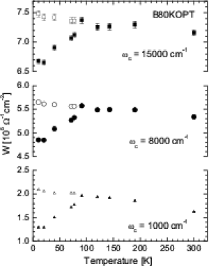
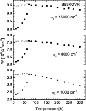
Figure 6: Spectral weight $W(T,\omega_{c})$ versus temperature for the underdoped (left), optimally doped (middle) and overdoped (right) samples, at different cutoff frequencies $\omega_{c}$ (full symbols). $\omega_{c}=1000$ cm^-1 (triangles); 8000 cm^-1 (circles); and 15000 cm^-1 (squares). Open symbols are obtained by adding the superfluid weight $W_{s}(T)$ to the spectral weight $W(T<T_{c})$. In the left panel, the dotted lines show approximately the expected location of the open symbols if all the spectral weight was removed from low energy states (see text), and the solid line at 8000 cm^-1 shows the average value (between 10 K and 50 K) of the open symbols. In all the curves, the absolute value of the spectral weight is subject to a systematic error of the order of $15-20$%. The errors in the relative variations of the spectral weight are indicated either by the size of the symbols or by the error bars.

The error incurred by doing so can be estimated as follows. Figure 6 displays the temperature dependence, from 300 K down to 10 K, of the spectral weight $W(\omega_{c},T)/W(\omega_{c},300{\rm K})$, for three selected integration ranges, according to Eq. 1. At $\omega_{c}=1000$ cm^-1, for example, the spectral weight exhibits a significant increase as the temperature is lowered, and could therefore keep increasing in the superconducting state. Hence $W(T_{A})$ is most likely to give too small an estimate for $W_{n}(T_{B})$ at $T<T_{c}$, in this energy range. To get a better insight of this possible underestimate, the superfluid weight $W_{s}(T)$ was added to the spectral weight $W(T_{B})$ (open symbols in Fig. 6), at each frequency $\omega=\omega_{c}$ (for temperatures $T<T_{c}$). These points represent how $W_{n}(T_{B})$ would evolve at $T<T_{c}$ if all the superfluid weight were accumulated from the spectral range $0^{+}\to\omega_{c}$. One can try to infer the evolution of $W_{n}(T_{B})$ from the temperature behavior of the data points close to, but still above, $T_{c}$. For example, for the underdoped sample, at $\omega_{c}=1000$ cm^-1, one could infer an increase of $\sim 4$% of $W_{n}(T_{B})$ from $T_{c}$ down to 10 K. This translates into an absolute error of about 0.3 in the value of the FGT sum rule at this frequency.

Such estimates have been performed for a number of cut-off frequencies starting from 100 cm^-1. The error in the FGT sum rule is the largest and most ill-defined at low frequencies (where only a rough estimate is possible), but becomes negligible at 5000 cm^-1 and above, where the changes with temperature of the normal-state spectral weight should be approximately 10 times smaller than at 1000 cm^-1 and present a smoother behavior when crossing $T_{c}$. At 15000 cm^-1 and beyond (Fig. 6), the normal-state spectral weight is constant for $T<170$ K, meaning that the redistribution of spectral weight in the normal state lies within this range of frequencies. Above 5000 cm^-1, the uncertainties that we have to deal with are those due to the error in the relative change of the measured reflectivity with temperature, to the fitting accuracy, and to the determination of $W_{s}$. The latter two uncertainties are not independent and must be calculated self-consistently. They yield an upper bound of 15 %–20 % in the uncertainty on the evaluation of $\Delta W/W_{s}$, for all frequencies. All uncertainties are then represented by the error bars in Fig. 5.

¿From figure 6 it is clear as well that any other choice of a normal-state temperature $T_{A}\geq T_{c}$ can only increase the violation of the FGT sum rule.

Another point that might be considered is whether, and how, the possible existence of a very low frequency mode, below the experimental window of the infrared spectroscopy, could give rise to an effect on the FGT sum rule as the one observed in this work. If such mode exists and could not be unveiled by the data analysis, then it would affect the evaluation of the normal and superconducting spectral weights, and/or of the superfluid density. Assuming that such mode has a simple Lorentzian form, one can straightforwardly show that its effect on the evaluation of the violation of the FGT rule is at worst $\sim\Delta\epsilon\times(\Omega_{\textsc{t}}/\Omega_{\textsc{l}})^{2}$, where $\Delta\epsilon$ is the oscillator strength of the mode, $\Omega_{\textsc{t}}$ its frequency, and $\Omega_{\textsc{l}}$ the London frequency of the system. Taking $\Omega_{\textsc{t}}\lesssim 10$ cm^-1 (our measurements begin at 30 cm^-1), and $\Omega_{\textsc{l}}\approx 2500$ cm^-1 (for our underdoped sample), one obtains that an effect of the order of 20% on the FGT sum rule (our experimental observation) would need a mode with an oscillator strength $\Delta\epsilon\gtrsim 10^{4}$. If such gigantic oscillator strengths can be observed in insulating materials,Blumberg-BB they are physically unreasonable in metallic systems where the low-frequency reflectivity is nearly unity. We have additionally performed numerical simulations on our data to evaluate more accurately the possible effect of such modes. The result is that, even if a very-low frequency mode with $\Delta\epsilon\sim 10^{4}$ is included in the fittings, but the accuracy of the fit in the measured experimental range is kept constant, the associated effect in the FGT sum rule is at most of the order of 10% at frequencies up to $\sim 5000$ cm^-1, and negligible or slightly negative (the sum rule violation is enhanced) beyond.

For the underdoped sample, the violation of the sum rule, with $\Delta W/W_{s}=0.80\pm 0.15$ at 8000 cm^-1, is then clearly established. Within the error bars, the sum rule is exhausted in this sample above 16000 cm^-1. The fact that the superfluid involves high energy states is compatible with the plot below $T_{c}$ of the sum of the spectral weight at finite frequency and the superfluid weight (open symbols in Fig. 6). Unlike the overdoped sample, where at 1000 cm^-1 the spectral weight of the condensate already balances the spectral weight lost up to this frequency, in the UD sample the superfluid spectral weight exceeds the loss at 1000 cm^-1 (by roughly a factor of 2). This corresponds to $\Delta W/W_{s}$ being of order 50 % at this energy, consistent with the data of Fig.  5 including the error bars. At 8000 cm^-1, for the UND sample, the open symbols of Fig. 6 are consistently above the normal-state spectral weight, suggesting that there is still some spectral weight coming from higher energy, and consistent with the value for the violation of the sum rule at this frequency.

III.2 Violation of the sum-rule, change of kinetic energy and pairing mechanism

One interpretation of the sum rule violation can be made in the context of the tight-binding Hubbard model. The relation between the spectral weight over the conduction band and the kinetic energy $E_{kin}$ per copper site yields:vdMTrieste

$$\frac{\Delta W}{W_{s}}+\frac{4\pi c}{137\hbar}\frac{a^{2}}{V}\frac{1}{\Omega_{L}^{2}}(E_{kin,n}-E_{kin,s})=1$$ (2)

where $a$ is the (average) lattice spacing in the plane and $V$ is the volume per site (SI units). This relation means that a breakdown of the FGT sum-rule up to an energy $\hbar\omega_{c}$ of the order of the plasma frequency ($\sim 1$ eV for Bi-2212) is related to a change in the carrier kinetic energy $\Delta E_{k}=E_{kin,n}-E_{kin,s}$, when entering the superconducting state. According to our results in the underdoped sample (Fig. 5), $\Delta W/W_{s}=0.80\pm 0.15$ at 1 eV and $\Omega_{L}^{2}=6.52\times 10^{6}$ cm^-2, which yields $\Delta E_{k}=(0.85\pm 0.2)$ meV per copper site. This would be a huge kinetic energy gain, $\sim 10$ times larger than the condensation energy $U_{0}$. For optimally doped Bi-2212, $U_{0}\simeq 1$ J$/$g-at $\approx 0.08$ meV per copper site.Loram

A similar, though more robust estimate of the kinetic energy gain for the underdoped sample can be made from figure 6 by taking into account the temperature evolution of the spectral weight in the normal and superconducting states, and not just the difference between the spectral weights at 100 K and 10 K. At 8000 cm^-1, when the superfluid weights are included below $T_{c}$ (open symbols), figure 6 represents the intraband spectral weight, hence $-E_{k}$, as a function of temperature. Below 170 K and above the resistive transition at 100 K, the normal-state spectral weight for the underdoped sample levels-off (its average value is represented by the dotted line), and we observe a clear excess of spectral weight in the superconducting state with respect to the average normal-state spectral weight. Taking as well the average of the low-temperature superconducting spectral weight (solid line through the open symbols) we find $\Delta E_{k}=(0.83\pm 0.2)$ meV per copper site, in agreement with our estimate from the violation of the FGT sum rule. If we incorporate the two data points at 80 K and 75 K (within the resistive transition), we find $\Delta E_{k}=(0.5\pm 0.2)$ meV per copper site.Andres-Miami

Various scenarios are consistent with our results. Most of them (but not all) propose indeed a superconducting transition driven by an in-plane kinetic energy change: holes moving in an antiferromagnetic background,AFEk-1 ; AFEk-2 ; AFEk-3 hole undressing,Hirsch1-1 ; Hirsch1-2 ; Hirsch2 phase fluctuations of the superconducting order parameter in superconductors with low carrier density (phase stiffness),Eckl-PhaseFluctDEk and quasiparticle formation in the superconducting state.NormanPepin-QPFormation There is a quantitative agreement between our results and those of the hole undressing and quasiparticle formation scenarios. Other models have been recently discussed in order to account for these data.Benfatto-Model ; Stanescu-Model ; Ashkenazi-Model ; Carbotte-Model ; Wrobel-Model ; Kopec-Model

Recently, STM experiments in optimally doped Bi-2212 samples showed small scale spatial inhomogeneities, over $\simeq 14$ Å, which are reduced significantly when doping increases, and whose origin could be local variations of oxygen concentration.Davis Since the wavelength in the full spectral range is larger than 14 Å, the reflectivity performs a large scale average of such an inhomogeneous medium. The implications in the conductivity are still to be investigated in detail, but it is presently unclear how this could affect the sum rule.

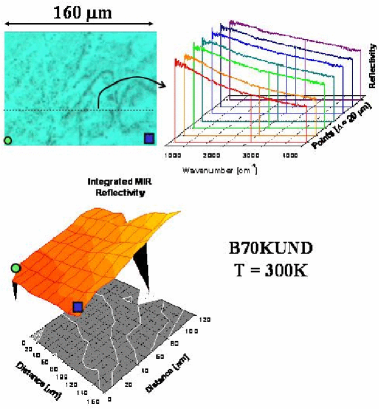
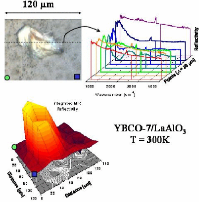
Figure 7: Left: infrared chart of the B70KUND sample. The picture of the scanned region (upper left corner) shows some sub-micronic defects. The reflectivity spectra along the dotted line (upper right corner) are identical, and the integrated reflectivity chart (lower left corner) is homogeneous. (The two peaks correspond to mechanical instabilities in the microscope sample holder during the measurements, and can not be reproduced). Right: infrared chart of a YBCO-7 sample, having surface defects larger than 10 $\mu$m. Note that the reflectivity spectra along the dotted line, and the integrated reflectivity chart, both show accidents clearly correlated with the surface defect seen on the picture.

IV CONCLUSIONS

In conclusion, we have found for the in-plane conductivity of the underdoped Bi-2212 a clear violation of the FGT sum rule at 1 eV, corresponding to a large ($\sim 20$ %) transfer of spectral weight from regions of the visible spectrum to the superfluid condensate. Within the framework of the tight-binding Hubbard model, this corresponds to a kinetic energy lowering of $\sim 0.5-1$ meV per copper site. The very large energy scale required in order to exhaust the sum rule in the underdoped sample cannot be related to a conventional bosonic scale, hence strongly suggests an electronic pairing mechanism.

V APPENDIX

V.1 Infrared microscopy characterizations

Even if infrared and visible spectroscopy measures the bulk optical properties of cuprates (the infrared skin-depth of Bi-2212 is $\gtrsim 3000$ Å), a flat surface of high optical quality in the whole measured spectral range is an important requirement for the accuracy in the measurement of the absolute value of the reflectivity. Besides checking our samples under an optical microscope, we characterized the mid-infrared optical quality of our films by infrared microscopy at room temperature, using the infrared microscope of the MIRAGE beamline at LURE (Orsay).MIRAGE In this microscope, the light being focussed on a point on the sample has been previously analyzed by a Fourier Transform spectrometer. In this way, the infrared reflectivity spectrum for each measured point is available. In our case, we worked at a spatial resolution of 20 $\mu$m. We then made, for each sample, scans over zones typically $160\times 160$ $\mu$m², recording for each measured point the spectrum in the $[500-4000]$ cm^-1 range.

Figure 7 illustrates the cases of a good (left) and a bad (right) optical quality in the mid-infrared [the figure in the right corresponds actually to the YBCO thin film, with a $T_{c}=90$ K]. We found, not surprisingly, that a defect whose size is comparable to the infrared wavelength ($\gtrsim 10$ $\mu$m), and that is easily spotted with the visible microscope (picture in Fig. 7, right), can perturb drastically the local reflectivity spectra. (We have not, on the other hand, found any case where a smooth region in the optical microscope was defective under the infrared microscope). If the ensemble of these infrared-defective regions represents a few percent of the total sample surface, then the average reflectivity of the whole surface will not accurately represent the intrinsic value of the absolute reflectivity of the sample (i.e., the average reflectivity over the whole surface will differ by more than 1% from the actual value of the reflectivity one would obtain with a sample of the same doping characteristics but with a surface free of defects). Our characterizations show as well that the infrared spectra are not sensitive to sub-micronic defects, whose size is comparable to the wavelengths in the visible (Fig. 7, left).

V.2 Sample selection

A first screening of the samples was done based on their resistive, optical-microscopy and $\mu$IR characteristics. We selected the samples showing a metallic behavior in the normal state, having the narrowest transitions ($\sim 20$ K to $\sim 10$ K for UND to OVR, respectively), homogeneous under the optical microscope, and displaying homogeneous $\mu$IR charts. The reflectivity spectra of the samples thus selected were adjusted to obtain their conductivities, using a fitting procedure that will be discussed in the next section. In this fitting procedure, the thickness of the sample enters as a parameter. Samples whose measured thickness differed by more than 15% (the accuracy of RBS measurements on Bi-2212) from the thickness needed to adjust the measured reflectivity were discarded. Samples showing abnormal electronic behavior (e.g., localized states at low frequency, or a temperature dependence of the low-frequency conductivity not matching the DC measurements) were discarded as well. At the end, three samples having passed confidently all the screenings, and spanning the three different doping regions, were selected for a thorough analysis. The critical temperatures (doping) of the selected films are 70 K (UND), 80 K (OPT) and 63 K (OVR).

The thickness of the films is an important issue: it is needed to deduce the intrinsic optical functions of the Bi-2212 despite the presence of a substrate which modifies the overall reflectivity. After the optical measurements were completed, the thickness of the B80KOPT and B63KOVR samples was directly verified by a second run of RBS measurements , yielding 395 nm and 270 nm ($\pm 30$ nm) respectively, in agreement with the thicknesses derived from fitting their reflectivities. The uncertainty of the RBS measurement (larger than 10%) is not quite satisfactory, since as discussed further, it is possible to change the assumed thickness within 10% and the incurred error bar is $\sim 10$%. The B70KUND sample was crucial, and the RBS measurement on a film grown under the same conditions (but on a MgO substrate) yielded 220 nm, already in agreement (within 10%) with the thickness deduced from the fit. We therefore decided to try and achieve a better accuracy using a TEM measurement, thus precluding a second RBS run. This attempt was unsuccessful.

V.3 Thin-films: extraction of the Bi-2212 optical functions

Among the various different models that we tried for a film on top of a substrate, we found that the best description of our raw reflectivity spectra is obtained by assuming that the light bouncing back and forth within the film interferes coherently and that the substrate has an infinite thickness (no light is reflected from its rear face). The typical thickness of our films being 3000 Å, that of the substrate $\sim 0.5$ mm, the refractive index of the Bi-2212 film (F) in the mid-infrared (around 800 cm^-1, for example) being $\eta_{\textsc{f}}\approx 5$ and that of the substrate (S) $\eta_{\textsc{s}}\sim 0.1-5$, one can deduce that, in this spectral range, the ratio “optical path $/$ wavelength in the medium” for a round-trip path of the light is about 0.24 for the Bi-2212, and $8-40$ for the substrate. On the other hand, even if the substrate is transparent in the near-infrared and the visible, its rear face in our films is not polished, so that the light is scattered from this face. The above-mentioned assumptions are thus largely justified on physical grounds.

The interfaces playing a role in our model are thus helium bath-film (HF) and film-substrate (FS). They are characterized by complex reflection [$r_{12}=(n_{1}-n_{2})/(n_{1}+n_{2})$] and transmission [$t=2n_{1}/(n_{1}+n_{2})$] coefficients from medium 1 (refractive index $n_{1}$) to medium 2 (refractive index $n_{2}$). The refractive index of the helium bath around the sample is 1. Denoting by $\rho$ the complex reflection coefficient of our films (the measured reflectivity being thus $R=|\rho|^{2}$), and by $\delta$ the thickness of the film, and assuming a coherent interference within the film and an infinite substrate, one easily finds

$$\rho=r_{\textsc{hf}}+\frac{t_{\textsc{hf}}t_{\textsc{fh}}r_{\textsc{fs}}A_{\textsc{f}}}{1-r_{\textsc{fs}}r_{\textsc{fh}}A_{\textsc{f}}},$$ (3)

where $A_{\textsc{F}}(\omega,\delta)=\exp[2i(\omega/c)\eta_{\textsc{f}}(\omega)\delta]$. Therefore, when the complex refractive indices of the film and the substrate (entering into the various coefficients $r$ and $t$) and the thickness of the film are known, one can describe the measured reflectivity $R$.

We have measured the reflectivity of a single crystal of SrTiO₃ for all the temperatures and spectral range relevant to our work. We have thus at hand the optical functions of the substrate. Hence, the measured reflectivity spectra can be adjusted by means of the Eq. 3 by simulating only the refractive index of the Bi-2212. The choice of the essay functions to simulate $\eta_{\textsc{f}}$ is arbitrary, provided the chosen functions obey causality (see next section). When the fitting is exact, this procedure yields the exact optical functions of the film alone, and the film thickness. The latter has been controlled by RBS measurements (see main text). The uncertainties arising from the accuracy of the fit are discussed in the next section.

V.4 Thin-film reflectivity: analysis of uncertainties and errors

If ${R(\omega),\omega\in\left[0,\infty\right)}$ is the complete and exact reflectivity spectrum of a material, then the phase $\theta(\omega)$ of the complex reflectance coefficient of the system can be deduced from a Kramers-Kronig transformation (TKK) on $R(\omega)$ alone:Wooten

$$\theta(\omega_{0})=-\frac{\omega_{0}}{\pi}\int_{0}^{\infty}\frac{\ln[R(\omega)/R(\omega_{0})]}{\omega^{2}-\omega_{0}^{2}}d\omega,$$ (4)

This relation arises solely from the assumption of a linear and causal response of the system to the electromagnetic excitation.

The knowledge of $R$ and $\theta$ allows the determination of any optical function $f(\omega)$ by means of simple algebraic relations. We will write

$$f(\omega)=f[R(\omega),\theta(\omega)].$$ (5)

It is evident, from (4) and (5), that if the reflectivity $R(\omega)$ of a given system is known, and if we can exactly fit this reflectivity with any arbitrary essay function obeying causality, then the optical functions issued from this essay function are mathematically identical to those issued from a Kramers-Kronig transformation of $R(\omega)$. In other terms, an exact fitting from zero to infinity with a causal function is completely equivalent to doing TKK.

Experimentally, the reflectivity is only known within a spectral range $[\omega_{a},\omega_{b}]$. Besides, the reflectivity is never measured with zero uncertainty, neither in absolute value nor in its relative (frequency- and/or temperature-) variations. These two facts affect the accuracy in the determination of the optical functions (either in the fitting or TKK cases), and are the departure point for the analysis of the uncertainties and errors in the determination of the optical functions of a system from its measured reflectivity. In the case of fitting, one additional source of error is the accuracy of the fitting within the measured frequency window.

The uncertainty in the determination of an optical function at a given frequency depends on the uncertainty on the determination of the reflectivity at all the frequencies, as seen from relation 4. Be $\Delta R(\omega)$ and $\xi(\omega)\equiv\Delta R(\omega)/R(\omega)$, respectively, the absolute and relative errors in the determination of the reflectivity. The questions at stake in the analysis of the errors in the optical functions are thus:

1. Given the maximum value $|\xi|_{\textrm{max}}$ that $\xi(\omega)$ can take in a frequency range, what is the maximum error expected in the determination of the optical functions?

2. How, in the calculation of the optical functions from the reflectivity, does the error $\xi(\omega)$ propagate to frequencies $\omega\prime\neq\omega$?

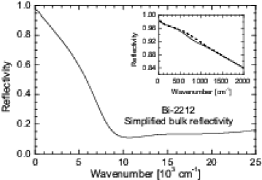
Figure 8: Simulated reflectivity for Bi-2212 in the normal state, in the spectral range $0-25000$ cm^-1, constructed from a superposition of a Drude plus various broad Lorentz oscillators. The inset shows a Gaussian “perturbation” (dashed spectrum) to this “exact” reflectivity, used as a model for a fitting or measure mismatch in the mid-infrared.

To answer these questions, let us call $\Delta\theta$ the error, due to $\Delta R$, in the determination of the phase of the reflectance coefficient. Assuming that $|\Delta R|$ and $|\Delta\theta|$ are small compared to unity (which is always true in the measured spectral range), then the relative errors in the determination of any optical function can be expressed in terms of $R$, $\theta$, $\xi$ and $\Delta\theta$ as:

$$\frac{\Delta f(\omega)}{f(\omega)}=C_{\xi}(\omega)\xi(\omega)+C_{\theta}(\omega)\Delta\theta(\omega).$$ (6)

The dimensionless factors $C_{\xi}$ and $C_{\theta}$ are different for the different optical functions of a given system. In particular, for the conductivity, it can be shown that $C_{\xi}\sim(1-R)^{-1}$. Besides, they have a complicated explicit dependence on $R(\omega)$ and $\theta(\omega)$, so that, for a given optical function, their frequency-dependencies are different for systems with different reflectivities. Hence, $\Delta f/f$ depends on the explicit form of the reflectivity spectrum, and the examination of the uncertainties in the determination of the optical functions has to be made on a case-by-case basis. While an analytical approach to the study of these uncertainties in the case of cuprates can be performed, the calculations involved are too lengthy (though simple; they can be found in reference Andres-Thesis ) and yield too crude results. For a system with a non-trivial reflectivity spectrum like Bi-2212, it is far more reliable to perform some numerical simulations and to compare them with the analytical studies.

Figure 8 shows a simplified typical reflectivity for Bi-2212. This reflectivity has been constructed by superposing a Drude and various broad Lorentz oscillators. It corresponds approximately to the reflectivity of an overdoped Bi-2212 sample in the normal state. Analyzing an overdoped-like reflectivity that is close to unity at low frequencies sets an upper limit, in this frequency range, to the errors incurred in the determination of the optical functions. Let us then define a “Gaussian perturbation” $\xi_{\textsc{g}}(\omega)$ (center $\omega_{c}$, half-width $\sqrt{2}\sigma$) to this exact reflectivity:

$$\xi_{\textsc{g}}(\omega)=\alpha\exp{[-\frac{(\omega-\omega_{c})^{2}}{2\sigma^{2}}]}.$$ (7)

This kind of perturbation represents reasonably well the type of errors expected when fitting the experimental reflectivity using Drude and broad Lorentz oscillators, as we have done in this work. We will take $\alpha=|\Delta R/R|_{\textrm{max}}=1$%, $\omega_{c}=800$ cm^-1 and $\sigma=200$ cm^-1, as an example of a fitting mismatch of 1% in the mid-infrared (inset of Fig. 8).

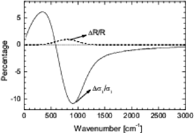
Figure 9: Relative uncertainty in the real conductivity (full line) introduced by a “Gaussian perturbation” on the mid-infrared reflectivity (dashed line). Note the change of sign of $\Delta\sigma_{1}/\sigma_{1}$, which was eventually neglected in the calculation of the error bars shown in the manuscript, leading to an overestimate of such error bars.

Numerical Kramers-Kronig transformations using the same kind of extrapolations for both reflectivities can then be performed to obtain the “exact” and “perturbed” conductivities, and then the relative error in the conductivity introduced by the perturbation. This relative error is shown in Fig. 9, where it is clear that $|\Delta\sigma_{1}/\sigma_{1}|_{\textrm{max}}\sim 5-10|\Delta R/R|_{\textrm{max}}$, and that the perturbation in the conductivity extends over a region of about 3 times that of $\Delta R/R$.

The latter example illustrates well the uncertainties endemic of a fitting procedure. Two other kinds of uncertainties play a role in the determination of the optical functions from reflectivity data, and are to be considered whichever method (TKK or fitting) is used for analyzing the data. These are: the error in the absolute measurement of the reflectivity, and the effect on the measured window of the (unknown) low- and high-frequency response of the system (the problem of the choice of extrapolations when doing TKK).

Analytical studies and numerical simulations Andres-Thesis show that, for a system like Bi-2212, and with an accuracy in the absolute measurement of the reflectivity of the order of 1% (our case), the associated uncertainties in the conductivity become important (20% or more) at frequencies below $\sim 100$ cm^-1. On the other hand, as this is a systematic error, it can be largely suppressed by comparing two conductivity curves of the same sample. This is precisely what is done in the evaluation of the FGT sum rule or in the calculation of the relative changes of spectral weight with temperature. Besides, the comparison between the extrapolated zero-frequency conductivity and the resistivity (Fig. 4) narrows the confidence range of the low-frequency conductivity.

As for the effects of the low- and high-frequency extrapolations, the conclusion of our analysis and simulations is that they can perturb the determination of the optical functions up to (at most) twice the first measured frequency and down to (at most) $1/3$ of the last measured frequency.

References

- (1) C.G. Olson et al., Science 245, 731 (1989).
- (2) C.G. Olson et al., Phys. Rev. B 42, 381 (1990).
- (3) J.C. Campuzano et al., Phys. Rev. Lett. 64, 2308 (1990).
- (4) D.S. Dessau et al., Phys. Rev. Lett. 71, 2781 (1993).
- (5) H. Ding et al., Phys. Rev. Lett. 76, 1533 (1996).
- (6) J. Mesot et al.,Phys. Rev. B 63, 224516 (2001).
- (7) D.N. Basov et al., Phys. Rev. B 63, 134514 (2001).
- (8) J. Corson et al., Phys. Rev. Lett. 85, 2569 (2000).
- (9) A.F. Santander-Syro et al., Phys. Rev. Lett. 88, 097005 (2002).
- (10) T. Timusk and B. Statt, Rep. Prog. Phys 62, 61 (1999).
- (11) A.V. Puchkov, D.N. Basov and T. Timusk, J. Phys. Condens. Matter 8, 10049 (1996).
- (12) R.A. Ferrell and R.E. Glover, Phys. Rev. 109, 1398 (1958).
- (13) M. Tinkham and R.A. Ferrell, Phys. Rev. Lett. 2, 331 (1959).
- (14) C. Renner et al., Phys. Rev. Lett 80, 149 (1998).
- (15) M. Randeria and J.C. Campuzano, cond-mat/9709107 (1997).
- (16) A.E. Karakozov, E.G. Maksimov and O.V. Dolgov, Solid State Commun., 124, 119 (2002).
- (17) D.N. Basov et al., Science 283, 49 (1999).
- (18) A.S. Katz et al., Phys. Rev. B 61, 5930 (2000).
- (19) J.E. Hirsch, Physica C 199, 305 (1992).
- (20) J.E. Hirsch, Physica C 201, 347 (1992).
- (21) J.E. Hirsch, F. Marsiglio, Physica C, 331, 150 (2000).
- (22) J.E. Hirsch, Phys. Rev. B 62, 14487 (2000).
- (23) J. Hirsch and F. Marsiglio, Phys. Rev. B 62, 15131 (2000).
- (24) M. Rübhausen et al., Phys. Rev. B 63, 224514 (2001).
- (25) H.J.A. Molegraaf et al., Science 295, 2239 (2002).
- (26) A.V. Boris et al, Science 304,708 (2004)
- (27) A.F. Santander-Syro et al., Europhys. Lett 62, 568 (2003).
- (28) M.R. Norman and C.Pépin, Phys. Rev. B 66, 100506(R) (2002).
- (29) Z.Z. Li, S. Labdi, A. Vaures, S. Megtert and H. Raffy. Proceedings of the Symposium A1 of the ICAM 91-EMRS. L. Correa, Editor. Elsevier, New York, 1992 (page 487).
- (30) Z. Konstantinovic, Z.Z. Li and H. Raffy, Physica B 259, 569 (1999).
- (31) P. Prieto et al., Surface Science 251, 712 (1991).
- (32) Z. Konstantinovic, PhD Thesis, Université de Paris-Sud (2001).
- (33) E.G. Maksimov, et al., Solid State Commun. 112, 449 (1999).
- (34) D. van der Marel et al., Optical signatures of electron correlations in the cuprates, Lecture Notes, Trieste miniworkshop “Strong Correlation in the high era”, ICTP, Trieste (Italy), 17-28 July 2000.
- (35) M.J. Holcomb et al., Phys. Rev. Lett. 73, 2360 (1994).
- (36) W. A. Little, K. Collins and M. J. Holcomb. J. Supercond. 12, 89 (1999).
- (37) M.A. Quijada et al., Phys. Rev. B 60, 14917 (1999).
- (38) J. Eckstein and H. Raffy, Private communications.
- (39) M. Norman, private communication.
- (40) G. Villard, D. Pelloquin and A. Maignan, Phys. Rev. B 58, 15231 (1998).
- (41) D. Di Castro et al., Physics C 332, 405 (2000).
- (42) C. Homes et al., Phys. Rev. B 69, 0024514 (2004).
- (43) S. Chakravarty, Eur. Phys. J. B 5, 337 (1998).
- (44) G. Blumberg et al., Science 297, 584 (2002).
- (45) J.W. Loram et al., Physica C 341-348, 831 (2000).
- (46) A. F. Santander-Syro, R. P. S. M. Lobo, and N. Bontemps, cond-mat/0404290.
- (47) J. Bonca, P. Prelovsek, and I. Sega, Phys. Rev. B 39, 7074 (1989).
- (48) E. Dagotto, J. Riera, and A.P. Young, Phys. Rev. B. 42, 2347 (1990).
- (49) T. Barnes et al., Phys. Rev. B 45, 256 (1992).
- (50) T. Eckl, W. Hanke and E. Arrigoni, cond-mat/0207425.
- (51) L. Benfatto et al., cond-mat/0305276.
- (52) T. Stanescu and P. Phillips, cond-mat/0301254.
- (53) J. Ashkenazi, cond-mat/0308153.
- (54) J. P. Carbotte and E. Schachinger, cond-mat/0404192.
- (55) P. Wrober, R. Eder and P. Fulde, J. Phys. Condens. Matter 15, 6599 (2003).
- (56) T. K. Kopec, Phys. Rev. B 67, 014520 (2003).
- (57) S.H. Pan et al., Nature 413, 282 (2001).
- (58) F. Polack et al. SPIE Proceedings on Accelerator-Based Sources of Infrared and Spectroscopic Applications. G.L. Carr and P. Dumas, Editors. Volume 3775, pages 13-21, 1999.
- (59) F. Wooten, Optical Properties of Solids, Academic Press (1972).
- (60) A.F. Santander-Syro, Electrodynamique dans l’état normal et supraconducteur de Bi2Sr2CaCu2O8+δ: étude par spectroscopie infrarouge-visible (2002). (In French. Available on line at http://www.espci.fr/recherche/labos/lps/thesis.htm).