Condensation of Cavity Polaritons in a Disordered Environment

Abstract

A model for direct two band excitons in a disordered quantum well coupled to light in a cavity is investigated. In the limit in which the exciton density is high, we assess the impact of weak ‘pair-breaking’ disorder on the feasibility of condensation of cavity polaritons. The mean-field phase diagram shows a ‘lower density’ region, where the condensate is dominated by electronic excitations and where disorder tends to close the condensate and quench coherence. Increasing the density of excitations in the system, partially due to the screening of Coulomb interaction, the excitations contributing to the condensate become mainly photon-like and coherence is reestablished for any value of disorder. In contrast, in the photon dominated region of the phase diagram, the energy gap of the quasi-particle spectrum still closes when the disorder strength is increased. Above mean-field, thermal, quantum and fluctuations induced by disorder are considered and the spectrum of the collective excitations is evaluated. In particular, it is shown that the angle resolved photon intensity exhibits an abrupt change in its behaviour, going from the condensed to the non-condensed region.

I Introduction

When the interaction between light and matter is strong, photons propagating in a dielectric can couple to excitons and form composite Bose particles known as polaritons hopfield . Since these composite bosons have a light mass, there has long been interest in the possibility that they might undergo Bose condensation at relatively high transition temperatures. While the concept of a Bose condensate of bulk polaritons has been discussed extensively keldysh ; snoke_book , in the open system, low-energy polaritons are merely long wavelength photons, which are not conserved haug . As a result, polaritons are unable to condense into the ground state making the bulk polariton condensate an intrinsically non-equilibrium phenomenon. However, providing the lifetime of the polaritons is long compared to the thermalization time, the confinement of the photons in a microcavity may allow for the development of a quasi-equilibrium condensate.

In recent years, improvements in the technology of semiconductor quantum wells has made the study of high-Q strongly-coupled planar microcavities almost routine for III-V, II-VI and some organic semiconductors weisbuch ; lesidang ; lidzey . Pumped both near resonance savvidis_baumberg_saba (i.e. the cavity is excited at a ‘critical’ angle) or non-resonantly lesidang ; huang ; deng (i.e. the system is excited at large angles), sharp superlinear increase of the low energy polariton photoluminescence has been observed.

Polaritons are characterised by a very short radiative lifetime (of the order of $\tau_{\text{leak}}\sim 3$ ps) due to leakage from the cavity. This has to be compared with the time scale to establish equilibrium with the lattice, $\tau_{\text{lattice}}$, and the equilibration time of the polaritons themselves, $\tau_{\text{polariton}}$; the former controlled largely by exciton-phonon scattering and the latter by exciton-exciton scattering processes. Dynamical (or quasi-equilibrium) condensation of polaritons can be reached when $\tau_{\text{polariton}}<\tau_{\text{leak}}<\tau_{\text{lattice}}$. Due to the ‘bottleneck effect’ tassone , thermalization of small momenta polaritons by acoustic phonons is suppressed, causing a slow relaxation of polaritons in the low energy state. This process is found to be strongly suppressed at higher values of the pump power where superlinear emission occurs tartakovskii . Recently, evidence of quasi-equilibrium condensation, where the polariton life time reaches the relaxation time, including second order coherence in the optical field, has been observed deng .

Within a bosonic picture involving tightly bound excitons, much work has been published on polariton dynamics under non-resonant excitation, e.g. by making use of a rate equation approach pol_dynamics . In this paper, we will focus on the signatures of the fermionic nature of polaritons when the excitation density increases. Here, the theoretical framework is not fully established even in the case of thermal equilibrium. The relative role of Coulomb forces (i.e. direct interaction between electron-hole pairs) and photon mediated interactions has not been studied. There is also an incomplete understanding of the effects of disorder, inelastic scattering and ‘decoherence’ phenomena, this being very important in drawing a distinction between polariton condensation and conventional lasing. Furthermore, previous theories, including those that incorporate effects due to disorder and decoherence, have been at the mean field level. Our aim here is to address all three of these issues.

I.1 Background

Beginning with the pioneering work of Keldysh and coworkers keldysh_kopaev_kozlov , the continuous transition between the Bose condensed and BCS-like phase of the equilibrium electron-hole system has been discussed within the framework of a mean-field theory characterised by an order parameter involving the coherent polarisation. Refinements of the mean-field theory by Comte and Nozières comte_nozieres to include the effects of screening provided a consistent theory of the electron-hole liquid and condensate phases. In recent years, considerable efforts have been made to explore the influence of light-matter interaction in the non-equilibrium electron system driven by an external phase coherent laser source — the optical Stark effect stark . However, only recently has the effect of quantum phase coherent coupling of photons and excitons in the closed system been addressed.

Cavity polaritons interact both directly via the Coulomb coupling of their excitonic part, and indirectly via occupancy constraints on the excitonic component, sometimes referred to as phase-space filling. Since polariton masses are typically very small, the coherence temperature increases rapidly with number density. Once the characteristic interaction energy, either the dipole coupling energy or the Coulomb interaction, is larger than the coherence temperature of free polaritons, one must use an interacting theory. If the density is still low enough that excitons are not strongly overlapping, an appropriate approximation is to treat the excitons as bosons with a short range repulsion, or equivalently as two level systems. However, if the exciton density is high enough that the excitons become unbound then the separate electron and hole (fermionic) degrees of freedom are recovered.

Note then that there are at least two and generally three crossovers as a function of increasing excitation: from a dilute gas of weakly interacting polaritons to a strong coupling regime, where nevertheless excitons are bound; then to a regime where the density of excitons is high enough that they unbind (and which may be weakly coupled to light, in the sense that the Rabi frequency is small in comparison to the kinetic energy). If, as is usual, the latter regime is one of weak coupling, nevertheless at high enough excitation one may reach a strong coupling regime where the optical field provides the largest scale in the problem. It is in the intermediate, fermionic, regime of weak coupling, that conventional semiconductor lasers operate laser_book .

Previous theoretical work has addressed the question of the existence of coherent, condensed polariton states in a simplified model. Taking just a single cavity photon mode, polariton condensation has been explored within the framework of an effective ‘zero-dimensional’ model in which excitons are trapped in isolated quantum dots paul . Treated as two-level systems, the Hamiltonian for the coupled exciton-photon system can be presented as a Dicke model. The model allows for an inhomogeneous broadening of the levels, while a quasi-equilibrium condition was imposed by fixing the total number of excitations. At the level of mean-field (which becomes exact when the number of exciton states coupled by the same microcavity field is large), the ground state of the polariton system can be written as a variational wave function. This wave function is a superposition of coherent states of the exciton and photon in which both the amplitude of the cavity field and the electron polarisation acquire a non-zero expectation value.

Within the same two-level system model, the effect of decoherence processes have recently been studied in marzena . Treated again at the mean-field level, decoherence gradually suppresses the excitonic component of the order parameter, driving the system toward a gapless, weak-coupling regime similar to that of a conventional laser.

Although the zero-dimensional system does provide intuition about the collective properties of the polariton condensate, by its construction, it is not able to discriminate between the BEC and BCS-like character of the condensate phase in the low and high density limits. Furthermore, the restriction of the model to a single cavity photon mode does not allow for the consideration of fluctuations and dispersion of the excitations in the polariton condensate phase. Finally, in the two-level formulation, Coulomb interaction is not considered self-consistently, and both at mean-field level and beyond mean-field, the coherent polarisation and the coherent photon field are locked together. Among other consequences, this means that in this model the screening of Coulomb interaction by an increase of the density of excitations cannot be taken into account. On the other hand, such an effect is mimicked by the fermionic space filling effect, which also has the result of increasing the photon component at high excitation levels.

In the following, we will tune the strength of the light-matter interaction so as to explore the interplay of exciton and polariton condensation in a quasi two-dimensional microcavity system. Here, in contrast to the localised exciton theory, one can expect weak potential disorder to impact strongly on the integrity of the condensate phase zittartz . Therefore, to keep our discussion general, we will include the symmetry-breaking effect of a weak potential disorder on the condensate. Although the mean-field theory has the capacity to describe the entire continuous interpolation between the low density BEC phase and the high density BCS-like phase, for simplicity, we will limit our analysis of the mean-field theory and fluctuations to the high density phase.

I.2 Model

The many-body Hamiltonian for the coupled electron-hole/photon system can be separated into constituent components according to

$$\hat{\mathcal{H}}-\mu\hat{N}_{\text{ex}}=\hat{\mathcal{H}}_{\text{ei}}+\hat{\mathcal{H}}_{\text{dis}}+\hat{\mathcal{H}}_{\text{ph}}+\hat{\mathcal{H}}_{\text{int}}\;.$$ (1)

Here, $\hat{\mathcal{H}}_{\text{ei}}$ represents the interacting Hamiltonian of the electron and hole degrees of freedom in a semi-conducting quantum well, while $\hat{\mathcal{H}}_{\text{dis}}$ describes the random potential generated by quenched impurities and lattice defects. $\hat{\mathcal{H}}_{\text{ph}}$ denotes the Hamiltonian associated with the cavity photons and finally $\hat{\mathcal{H}}_{\text{int}}$ represents the exciton-photon dipole coupling interaction.

Following the notation introduced in Ref. zittartz and adopting an ‘electron picture’ in which $b_{{\mathbf{p}}}$ and $b_{{\mathbf{p}}}^{\dagger}$ ($a_{{\mathbf{p}}}$ and $a_{{\mathbf{p}}}^{\dagger}$) represent the annihilation and creation operators of an electron with momentum ${\mathbf{p}}$ in the conductance (valence) band (see Fig. 1), the Hamiltonian for a direct band-gap semiconductor is given by

$$\hat{\mathcal{H}}_{\text{ei}}=\sum_{{\mathbf{p}}}\xi_{{\mathbf{p}}}\left(b_{{\mathbf{p}}}^{\dagger}b_{{\mathbf{p}}}+a_{{\mathbf{p}}}a_{{\mathbf{p}}}^{\dagger}\right)\\ +\displaystyle\frac{1}{2}\sum_{{\mathbf{q}}\neq 0}v({\mathbf{q}})\left(\rho_{{\mathbf{q}}}\rho_{-{\mathbf{q}}}-\sum_{{\mathbf{p}}}b_{{\mathbf{p}}}^{\dagger}b_{{\mathbf{p}}}-\sum_{{\mathbf{p}}}a_{{\mathbf{p}}}a_{{\mathbf{p}}}^{\dagger}\right)\;,$$

where $\rho_{{\mathbf{q}}}=\sum_{{\mathbf{p}}}(b_{{\mathbf{p}}+{\mathbf{q}}}^{\dagger}b_{{\mathbf{p}}}-a_{{\mathbf{p}}}a_{{\mathbf{p}}+{\mathbf{q}}}^{\dagger})$ is the total electron density operator. Here, for simplicity, we suppose that the electrons are spinless. Taking the middle of the gap as the energy reference, we assume a parabolic conduction and valence band of particles

$$\xi_{{\mathbf{p}}}=\displaystyle\frac{{\mathbf{p}}^{2}}{2m}-\displaystyle\frac{\mu-E_{g}}{2}\equiv\displaystyle\frac{{\mathbf{p}}^{2}}{2m}-\varepsilon_{F}\;,$$ (2)

where, for simplicity, we have assumed the electrons and holes exhibit the same effective mass, $m$. At the level of mean-field, one can confirm that this assumption is innocuous and corresponds to replacing the effective mass with the double of the reduced mass. In contrast, deviation from parabolicity in the physical system impairs the capacity for perfect nesting of the Fermi surface and reduces the potential for pair correlation. Finally, for convenience, we have introduced in Eq. (2) the concept of an effective Fermi energy $\varepsilon_{F}\equiv p_{F}^{2}/2m=(\mu-E_{g})/2$, which, along with the chemical potential $\mu$, is determined self-consistently as a non-trivial function of the total number of excitations in the system (5) (see later in section III.1).

In addition to the lattice potential, the electrons and holes experience a Coulomb interaction. In the high density regime $\rho_{el}a_{0}^{2}\gg 1$, where $\rho_{el}=p_{F}^{2}/4\pi$ denotes the areal density of the particles, (i.e. when the the excitonic Bohr radius $a_{0}=2\epsilon_{0}/e^{2}m$ is much larger than the average distance between electron and holes $1/\sqrt{\rho_{el}}$), the Coulomb interaction is screened due to both electrons and holes zittartz ; comte_nozieres :

$$v({\mathbf{q}})=\displaystyle\frac{4\pi e^{2}}{\epsilon_{0}({\mathbf{q}}^{2}+\kappa^{2})}\;.$$

In the two-dimensional system, the screening length is approximately set by the Bohr radius $1/\kappa=a_{0}$. Hence, in this limit, the Coulomb interaction can be replaced by a short range contact interaction zittartz ,

$$\sum_{{\mathbf{p}}^{\prime}}v({\mathbf{p}}-{\mathbf{p}}^{\prime})\Big{|}_{|{\mathbf{p}}^{\prime}|=p_{F}}\simeq\begin{cases}\bar{V}&|p_{F}-p|<\kappa\\ 0&|p_{F}-p|>\kappa\;,\end{cases}$$

with a strength given by the angular average over the Fermi surface

$$\bar{V}=\operatorname{\mathcal{R}y}a_{0}^{3}\displaystyle\frac{8\pi}{\sqrt{1+(2p_{F}a_{0})^{2}}}\;.$$ (3)

Here $\operatorname{\mathcal{R}y}=e^{2}/2\epsilon_{0}a_{0}$ denotes the Rydberg energy associated with the exciton and sets the characteristic energy scale of the interaction. Therefore, as a consequence of the screening, an increase in the total number of electronic excitations leads to a reduction in the effective strength of the Coulomb interaction. Notice that, although the condensed state may have a gap, we shall be discussing the dense limit, where the coherence length is much longer than $1/\kappa$, and so this will not influence the important short range part of the potential.

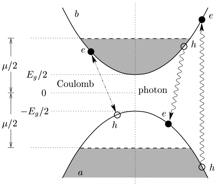
Figure 1: Schematic picture of the valence ($a$) and conductance ($b$) band, and the interactions included in the model (1).

To incorporate the effect of disorder, we suppose that the electron-hole system is subject to a generic weak impurity potential,

$$\hat{\mathcal{H}}_{\text{dis}}=\int d{\mathbf{r}}\;\left[U_{b}({\mathbf{r}})b^{\dagger}({\mathbf{r}})b({\mathbf{r}})+U_{a}({\mathbf{r}})a^{\dagger}({\mathbf{r}})a({\mathbf{r}})\right]\;.$$

Naively, since the electrons and holes carry opposite charge, their response to potential impurities should be equal in magnitude and opposite in sign. However, differences in the dielectric properties of the conduction and valence band electrons, combined with the potential asymmetry imposed by the quasi two-dimensional geometry, implies that the potentials $U_{a}$ and $U_{b}$ are not perfectly anticorrelated. Furthermore, there are mechanisms of disorder such as variations in the width of the quantum well through atomic terracing, strain fields, etc., that act on electrons and holes with the same sign. Therefore, in the following, we will suppose that a generic disorder potential is comprised of two channels: A potential $U_{n}({\mathbf{r}})\equiv[U_{b}({\mathbf{r}})-U_{a}({\mathbf{r}})]/2$ which acts symmetrically as a ‘charge-neutral’ potential and, as we will see, does not effect the integrity of the condensate phase. A second, statistically independent, potential $U_{c}({\mathbf{r}})\equiv[U_{b}({\mathbf{r}})+U_{a}({\mathbf{r}})]/2$ acts as an asymmetric ‘charged’ component, and presents a pair-breaking perturbation which gradually destroys the excitonic condensate. As mentioned above, its effect in the dense exciton system on the integrity of the exciton insulator phase has been explored in an early work by Zittartz zittartz . In both cases, we will suppose that the potentials $U_{n,c}$ are drawn at random from a Gaussian white-noise distribution, with zero mean, and variance given by

$$\langle U_{n,c}({\mathbf{r}}_{1})U_{n,c}({\mathbf{r}}_{2})\rangle=\displaystyle\frac{1}{2\pi\nu\tau_{n,c}}\delta({\mathbf{r}}_{1}-{\mathbf{r}}_{2})\;,$$ (4)

where $\tau_{n}$ and $\tau_{c}$ are the associated scattering times, and $\nu=m/2\pi$ is the two-dimensional density of states of the spinless electron system. Restricting attention to the high density phase, setting $\varepsilon_{F}\tau_{n,c}\gg 1$, we will further suppose that the impurity potential impose only a weak perturbation on the electron and hole degrees of freedom, allowing therefore the dynamics to be treated quasi-classically. This completes the description of the electron-hole system.

Free photons in the cavity are described by the microscopic quasi two-dimensional Hamiltonian

$$\hat{\mathcal{H}}_{\text{ph}}=\sum_{{\mathbf{p}}}\psi_{{\mathbf{p}}}^{\dagger}\left[\omega({\mathbf{p}})-\mu\right]\psi_{{\mathbf{p}}}\;,$$

where their dispersion, $\omega({\mathbf{p}})=\sqrt{\omega_{c}^{2}+(c{\mathbf{p}})^{2}}$, is quantised in the direction perpendicular to the plane of the cavity mirrors, $\omega_{c}=c\pi j/L_{\text{m}}$, where $L_{\text{m}}$ denotes the distance between the mirrors, and $j\in\mathbb{Z}$. In the following, we will suppose that the electron-hole system engages just a single sub-band for which $\omega_{c}\neq 0$. In practice, providing the sub-band separation is substantially larger than the quasi-particle energy gap that develops in the electron-hole system, neighboring sub-bands can be safely neglected.

Finally, in the dipole or ‘rotating-wave’ approximation, the photons are assumed to be coupled to the electron-hole system through a local interaction,

$$\hat{\mathcal{H}}_{\text{int}}=g\int d{\mathbf{r}}\left[\psi({\mathbf{r}})b^{\dagger}({\mathbf{r}})a({\mathbf{r}})+\text{h.c.}\right]\;.$$

Here, terms which do not conserve the number of excitations (i.e. the ones describing spontaneous creation or annihilation of a photon and an exciton) have been neglected. On one hand, we expect this approximation to be valid in the weak coupling limit between photon and matter, where these additional terms can be ‘integrated out’, giving a small ‘renormalisation’ of the single particle electronic and photonic dispersion laws. At the same time, since we are dealing with a system where the temperature is much smaller than the photon frequency, we can neglect the tiny spontaneous population that would be generated by these non-resonant terms.

To mimic the effect of the external photon source, we suppose that the electron-hole/photon system is held in quasi-equilibrium by tuning the chemical potential $\mu$ in (1) to fix the total number of excitations

$$\hat{N}_{\text{ex}}=\sum_{{\mathbf{p}}}\psi^{\dagger}_{{\mathbf{p}}}\psi_{{\mathbf{p}}}+\displaystyle\frac{1}{2}\sum_{{\mathbf{p}}}\left(b^{\dagger}_{{\mathbf{p}}}b_{{\mathbf{p}}}+a_{{\mathbf{p}}}a^{\dagger}_{{\mathbf{p}}}\right)\;.$$ (5)

However, how the system chooses to portion the excitations between the electron-hole and photon degrees of freedom depends sensitively on the properties of the condensate.

This completes the formal construction of the microscopic many-body Hamiltonian. In order to explore the mean-field content and the collective excitations of the light-matter system, we will draw on the theory of the weakly disordered superconductor. Using conventional field theoretic methods, we will show that the low-energy properties of the system can be cast in the framework of an effective field theory with an action of non-linear sigma-model type efetov . Partitioning our discussion into properties of the mean-field content of the theory and the role of fluctuations, we will focus on the phase diagram of the system as a function of density and disorder on one side, and the nature of the collective excitations on the other. Since the field theory technology disguises much of the physical content, we will close the introduction with an overview of the findings of the mean-field theory. As well as summarising the main results, it will provide a useful prospective for the formal analysis.

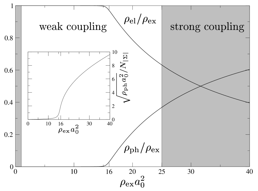
Figure 2: Relative number of (total) electrons $n_{\text{el}}=\rho_{\text{el}}/\rho_{\text{ex}}$ and (condensed) photons $n_{\text{ph}}=\rho_{\text{ph}}/\rho_{\text{ex}}$ are plotted against $\rho_{\text{ex}}a_{0}^{2}$ for fixed values of the coupling constants $\tilde{g}=1$ and $\lambda_{c}=10$ and for $d=200$. Note that, for $\rho_{\text{ex}}a_{0}^{2}>25$, the system enters a strong coupling regime, where our model cannot be applied. In the inset, the number of photons $\rho_{\text{ph}}a_{0}^{2}$ is compared with the number of electrons in the condensate, $N_{|\Sigma|}=|\Sigma|\nu a_{0}^{2}$ (see Eq. (21)). For $\rho_{\text{ex}}a_{0}^{2}>d/4\pi\simeq 16$, the excitations in the condensate are dominated by photons.

In the high density regime, the mean-field content of the action will be shown in section III to be insensitive to the ‘neutral’ component of the disorder potential, $U_{n}({\mathbf{r}})$, a manifestation of the Anderson theorem in the exciton context. This reproduces the mean-field thermodynamic properties of a system subject only to a ‘charged’ weakly disorder potential, $U_{c}({\mathbf{r}})$. By analysing these mean-field equations, the generalisation of those derived by Zittartz zittartz for the exciton insulator system, we will describe the rearrangement of the ground state due to condensate formation. In particular, we will show that the condensate of the polariton system is characterised by an order parameter which engages the combination of the phase locked polarisation and photon amplitudes. The mean-field phase diagram (see Fig. 3) can be characterised in terms of the total density of excitations, $\rho_{\text{ex}}a_{0}^{2}$, the disorder strength $\xi=1/\tau_{c}\operatorname{\mathcal{R}y}$ and the following dimensionless material parameters, respectively the coupling to the photon field and the Coulomb coupling strength (see expression (3)):

$$\begin{split}\tilde{g}&=g\sqrt{\displaystyle\frac{\nu L^{2}}{\operatorname{\mathcal{R}y}}}\\ \tilde{g}_{c}(x)&=g_{c}\nu L^{2}=\displaystyle\frac{\lambda_{c}}{\sqrt{1+4(d-x)}}\;.\end{split}$$ (6)

Here, the constant of proportionality $\lambda_{c}=4a_{0}/L_{\perp}$ depends on the thickness $L_{\perp}$ of the quantum well, $x=(\omega_{c}-\mu)/\operatorname{\mathcal{R}y}$ denotes the characteristic energy separation between the photon band edge and the chemical potential (measured in units of the Rydberg), and $d=(\omega_{c}-E_{g})/\operatorname{\mathcal{R}y}>0$. Note that, as in BCS theory, $g_{c}$ scales with the volume, i.e. in the thermodynamic limit $g_{c}L^{2}$ is finite while, by contrast, $g$ scales with the square root of the volume, i.e. $g^{2}L^{2}$ is finite.

When the density $\rho_{\text{ex}}a_{0}^{2}$ is low, the majority of excitations are invested in electrons and holes (see figure 2) and therefore, as the density increases, the chemical potential rises linearly. Here, providing the density is large enough to keep the particles unbound, the condensed phase is reminiscent of the exciton insulator one, even if a small fraction of photons do contribute to the condensate (see the inset of figure 2). Eventually, as the chemical potential approaches the band edge, $\omega_{c}$, the photons are brought into resonance and the character of the condensate changes abruptly. Here, the excitations become increasingly photon-like, with $\rho_{\text{ex}}a_{0}^{2}$ diverging exponentially when the chemical potential converges on $\omega_{c}$. At the same time, screening suppresses the excitonic coupling constant, determining the majority of the excitation in the condensate to acquire a photon-like character. This is clearly shown in figure 2, where the normalised number of total electrons $\rho_{\text{el}}/\rho_{\text{ex}}$ and photons $\rho_{\text{ph}}/\rho_{\text{ex}}$ (see Eq. (20)) are plotted as a function of the density of excitations. In the inset of the picture, instead, the fraction of photons to excitons in the condensate (for the exact definition, see later on, Eq. (21)) clearly shows an abrupt growth as the density of excitations in increased above the value $d/4\pi$, which we will see to coincide with the maximum density which can be reached at $\mu=\omega_{c}$ in absence of photons.

Staying at the level of mean-field, the ‘charged’ component of the disorder potential presents a symmetry breaking perturbation which depletes the excitonic component of the condensate. As such, its effect on the condensate depends sensitively on the density of excitations. When $1<\rho_{\text{ex}}a_{0}^{2}<d/4\pi$, the condensate has a particle-hole character and the phase diagram (Fig. 3) mimics the behaviour of the symmetry broken exciton insulator zittartz – and therefore of a superconducting system in presence of magnetic impurities. When the scattering rate $\tau_{c}$ is comparable to the value of the unperturbed order parameter, the system enters a gapless phase before the condensate is extinguished altogether. At larger densities, the condensate becomes photon-dominated and therefore robust against any value of the disorder potential. Interestingly, however, the residual effect of the disorder exposes a substantial region of the phase diagram where the system is gapless. Here, the condensate acquires all of the conventional characteristics of a semiconductor laser — i.e. a substantial coherent optical field, but a gapless spectrum of electron-hole pairs with negligible electronic polarisation sclaser . Once again, at sufficiently large densities, the system enters a strong coupling regime, where the validity of the model becomes doubtful.

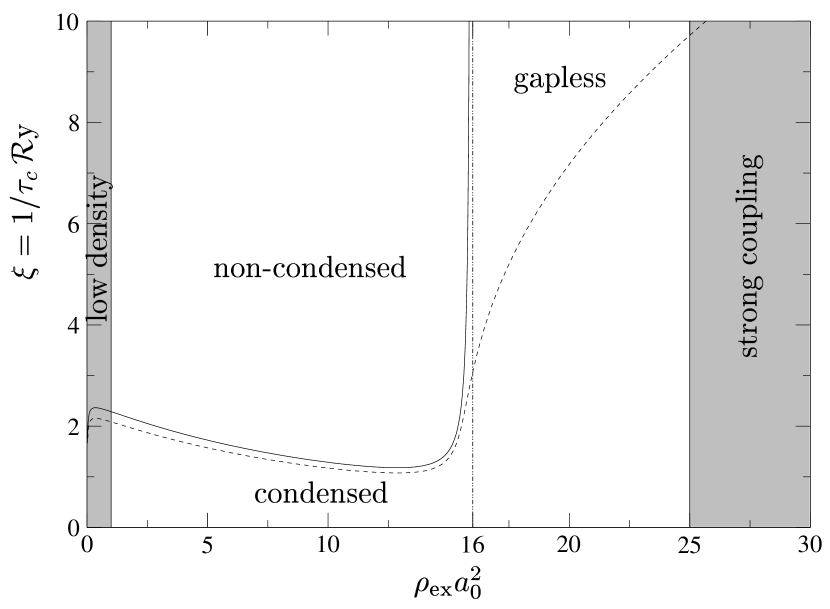
Figure 3: Mean-field phase diagram for $\tilde{g}=1$, $\lambda_{c}=10$ and $d=200$; $\rho_{\text{ex}}a_{0}^{2}$ represents the excitation density, while $\xi=1/\tau_{c}\operatorname{\mathcal{R}y}$ the disorder strength.

This completes our summary of the mean-field content of the theory. The remainder of the paper is organised as follows. In the next section, we develop a field theory of the weakly disordered polariton system. Focusing on the saddle-point approximation, in section III we elaborate and expand our discussion of the mean-field content of the model. Using these results as a platform and exposing analogies with the symmetry broken superconducting system, in section IV the attention is then turned to the impact of thermal, quantum and disordered driven fluctuations. Here, we explore the spectrum of the collective excitations and, in particular, we discuss how the transition to the condensed phase provide a signature in the photoluminescence. Finally, in section V, we conclude.

II Path Integral Formulation

The development of a low-energy field theory of the weakly disordered exciton-light system mirrors closely the quasi-classical theory of the disordered superconductor. By presenting the quantum partition function of the many-body system as a coherent state path integral, the ensemble or impurity averaged free energy can be cast in terms of a replicated theory. At the level of the mean-field theory, this approach is equivalent to the self-consistent Hartree-Fock treatment where the impact of disorder is treated in the self-consistent Born approximation. Using the mean-field result as a platform, the field theoretic formulation provides the means to develop a field theory of the low-energy excitations of the polariton condensate.

The quantum partition function $\mathcal{Z}=\operatorname{tr}[e^{-\beta(\hat{\mathcal{H}}-\mu\hat{N}_{\text{ex}})}]$, where $\beta=1/k_{\text{\sc{b}}}T$ is the inverse temperature, can be expressed as a coherent state path integral over fermionic and bosonic fields. To facilitative impurity averaging of the free energy over the disorder potentials (4), it is convenient to engage the ‘replica trick’ edwards_anderson ,

$$F=-\displaystyle\frac{1}{\beta}\langle\ln\mathcal{Z}\rangle=-\displaystyle\frac{1}{\beta}\lim_{n\to 0}\displaystyle\frac{\langle\mathcal{Z}^{n}\rangle-1}{n}\;.$$

Although the analytic continuation presents difficulties in treating non-perturbative structures, the technique can be applied safely to the mean-field and collective properties discussed in this work. Once replicated, a Hubbard-Stratonovich decoupling of the Coulomb interaction obtains the field integral for the quantum partition function

$$\mathcal{Z}^{n}=\int D(\psi^{*},\psi)\int D(\Sigma^{*},\Sigma)\;\int D(\phi^{\dagger},\phi)\,e^{-S_{\text{ph}}-S_{\Sigma}}\\ \exp\left[-\int_{0}^{\beta}d\tau\int d{\mathbf{r}}\;\phi^{\dagger}({\mathbf{r}},\tau)\left(\partial_{\tau}+\hat{H}\right)\phi({\mathbf{r}},\tau)\right]\;,$$ (7)

where, in order to lighten the notation, we have omitted the replica index carried by all of the fields. Here, $S_{\text{ph}}$ and $S_{\Sigma}$ correspond respectively to the bare photonic and excitonic components of the action,

$$S_{\text{ph}} =\int_{0}^{\beta}d\tau\sum_{{\mathbf{p}}}\psi_{{\mathbf{p}}}^{*}(\tau)\left[\partial_{\tau}+\omega({\mathbf{p}})-\mu\right]\psi_{{\mathbf{p}}}(\tau)$$ (8)

$$S_{\Sigma} =\displaystyle\frac{1}{g_{c}L^{2}}\int_{0}^{\beta}d\tau\int d{\mathbf{r}}\;|\Sigma({\mathbf{r}},\tau)|^{2}\;,$$ (9)

while, arranging the fermionic fields into a Nambu-like spinor $\phi^{\dagger}=(b^{\dagger},a^{\dagger})$ and $\phi=(b,a)^{\mathsf{T}}$, the (single-particle) action for the internal electronic degrees of freedom (which, with an abuse of terminology, we will later on refer to as ‘particle-hole’ components) takes the form reminiscent of the Gor’kov or Bogoliubov de-Gennes superconducting Hamiltonian,

$$\hat{H}=\left[\hat{\xi}_{\hat{{\mathbf{p}}}}+U_{n}({\mathbf{r}})\right]\sigma_{3}+U_{c}({\mathbf{r}})+\widehat{\Delta}\;.$$ (10)

Here, $\sigma_{i}$ represent Pauli matrices operating in the particle-hole subspace, and $\Delta=|\Delta|e^{i\chi}$ represents the complex ‘composite order parameter’

$$\widehat{\Delta}=\begin{pmatrix}0&\Sigma+g\psi\\ \Sigma^{*}+g\psi^{*}&0\end{pmatrix}=|\Delta|\sigma_{1}e^{-i\chi\sigma_{3}}\;.$$

involving both the polarisation $\Sigma$ and photon $\psi$ fields. Taking into account the contact nature of the screened Coulomb interaction, the coupling constant $g_{c}$ can be derived starting from the expression (3) and is given in Eq. (6). At the level of mean-field, the excitonic order parameter signals the development of the anomalous pairing amplitude

$$\Sigma({\mathbf{r}})=-g_{c}L^{2}\langle\text{g.s.}|b^{\dagger}({\mathbf{r}})a({\mathbf{r}})|\text{g.s.}\rangle\;,$$

while the ordinary Hartree-Fock pairings, $\langle\text{g.s.}|b^{\dagger}({\mathbf{r}})b({\mathbf{r}})|\text{g.s.}\rangle$ and $\langle\text{g.s.}|a({\mathbf{r}})a^{\dagger}({\mathbf{r}})|\text{g.s.}\rangle$, crucial in the low-density limit, effect only a small renormalisation of the single-particle energy $\xi_{{\mathbf{p}}}$. Restricting attention to the high density regime, such renormalisations can be neglected (or absorbed into a redefinition of the position of the band edge).

As noted above, the single-particle Hamiltonian for the electron and hole mirrors the structure of the quasi-particle Hamiltonian for a superconductor. In particular, in the absence of disorder, an electron of energy $\xi_{{\mathbf{p}}}$ in the valance band can pair with a hole of energy $\xi_{{\mathbf{p}}}$ in the conduction band. The development of a homogeneous order parameter $\Delta$ induces a gap in the quasi-particle density of states at the effective Fermi level $\varepsilon_{F}$. Already at this level, the insensitivity of the condensate to ‘neutral’ disorder $U_{n}$ is apparent: Even in the presence of the disorder potential, the electron with a single-particle energy can pair with a partner hole with the same energy and form a homogeneous condensate, a reflection of the Anderson theorem of superconductivity in the electron-hole system. By contrast, the symmetry breaking potential $U_{c}$ lifts the degeneracy of the electron and hole degrees of freedom and imposes a pair-breaking perturbation on the condensate. As a result, one expects a gradual depletion of the condensate. In fact, we will see later on in section III.2, when establishing the phase diagram, that, since photons are almost insensitive to the effect of disorder, only the ‘excitonic contribution’ to the condensate will be affected, while at very high densities, the photonic component will be able to restore coherence.

In principle, one could explore the mean-field content of the coupled system by developing a diagrammatic self-consistent Hartree-Fock approximation. However, in the following, we will be concerned with the impact of fluctuations on the integrity of the condensate phase. As well as thermal and quantum fluctuations, mechanisms of quantum interference affect the spectrum of quasi-particle excitations above the condensate. To properly accommodate these effects, it is helpful to construct an effective low-energy theory which encodes the diffusive character of the dynamics. To classify the different channels of interference, it is helpful to identify the symmetry properties of the coupled system.

As well as its invariance under the global gauge transformation

$$\phi \mapsto e^{i\chi^{\prime}\sigma_{3}/2}\phi \phi^{\dagger} \mapsto\phi^{\dagger}e^{-i\chi^{\prime}\sigma_{3}/2}$$

$$\Sigma \mapsto\Sigma\,e^{i\chi^{\prime}} \psi \mapsto\psi e^{i\chi^{\prime}}\;,$$ (11)

in the absence of the symmetry breaking potential $U_{c}$, the matrix Hamiltonian (10) exhibits the discrete particle-hole symmetry $\hat{H}=-\sigma_{2}\hat{H}^{\mathsf{T}}\sigma_{2}$. Its presence facilitates mechanisms of quantum interference which effect the low-energy properties of the quasi-particles excitations. Following a standard procedure (see, e.g., Ref. damian ), in order to properly take into account for the ‘soft diffusion modes’ associated with this symmetry, it is useful to double the field space setting

$$\Phi =\displaystyle\frac{1}{\sqrt{2}}\begin{pmatrix}\phi\\ \sigma_{2}{\phi^{\dagger}}^{\mathsf{T}}\end{pmatrix}_{\text{\sc{cc}}} \bar{\Phi} =\frac{1}{\sqrt{2}}\begin{pmatrix}\phi^{\dagger}&-\phi^{\mathsf{T}}\sigma_{2}\end{pmatrix}_{\text{\sc{cc}}}\;.$$

As a result, the fields $\Phi$ engage a total of $4\times n$ components (i.e. $n$ replica, particle-hole and ‘charge conjugation’ cc), while the redundancy implied by the field doubling imposes the symmetry relations $\Phi=\sigma_{2}\gamma\bar{\Phi}^{\mathsf{T}}$ and $\bar{\Phi}=-\Phi^{\mathsf{T}}\sigma_{2}\gamma^{\mathsf{T}}$, with $\gamma=-i\sigma_{2}^{\text{\sc{cc}}}$. It is important to note that the impact of the full charge-conjugation structure of the fields is manifest only in the mesoscopic fluctuation phenomena which effect only the low-energy quasi-particle excitations. In particular, such mechanisms of quantum interference do not effect the properties of the system at the level of the saddle-point or mean-field.

Cast in the form (7), the action mirrors closely that studied in the context of the disordered superconductor and, to identify the effective low-energy theory, one may draw on the existing literature. In particular, in the quasi-classical and dirty limits,

$$\varepsilon_{F}\gg\displaystyle\frac{1}{\tau_{n}}\gg\displaystyle\frac{1}{\tau_{c}},|\Delta|\;,$$ (12)

it has been shown damian ; lamacraft that the long-range properties of the system can be expressed in terms of an action of nonlinear $\sigma$-model type,

$$\langle\mathcal{Z}^{n}\rangle=\int D(\psi^{*},\psi)\int D(\Sigma^{*},\Sigma)e^{-S_{\text{ph}}-S_{\Sigma}}\int DQ\;e^{-S[Q]}\;,$$

where

$$S[Q]=\displaystyle\frac{\pi\nu}{8}\int d{\mathbf{r}}\operatorname{tr}\left[D(\nabla Q)^{2}\right.\\ \left.-4\left(\hat{\epsilon}\sigma_{3}\sigma_{3}^{\text{\sc{cc}}}-i\widehat{\Delta}\sigma_{3}\right)Q-\displaystyle\frac{1}{\tau_{c}}\left(\sigma_{3}\sigma_{3}^{\text{\sc{cc}}}Q\right)^{2}\right]\;.$$ (13)

Here, $D=v_{F}^{2}\tau_{n}/2$ represents the diffusion constant associated with the ‘neutral’ disorder, while the matrix field $Q({\mathbf{r}})=T({\mathbf{r}})\Lambda\sigma_{3}\sigma_{3}^{\text{\sc{cc}}}T^{-1}({\mathbf{r}})$ carries replica, time and internal (particle-hole and cc) indices, and the generators $T$ are compatible with the ‘charge-conjugation ’symmetry properties which $Q$ inherits from the dyadic product $\sigma_{3}\Phi\otimes\bar{\Phi}$. Qualitatively, the fluctuations of the matrix field Q encode the effect of long-range mechanisms of quantum interference.

Combined with the bare actions for the auxiliary fields (8) and (9), the non-linear $\sigma$-model action fully encodes the effect of weak disorder in the cavity polariton system. In the absence of the order parameter, the action describes the diffusive density relaxation of, separately, the electron and hole degrees of freedom. The development of the order parameter $|\Delta|$ describes the rearrangement of the ground state due to the formation of the polariton condensate. Finally, scattering in the channel of the ‘charged’ disorder potential projects out the diffusion modes which act coherently on the particle-hole degrees of freedom. In order to explore the capacity of the system to undergo condensation, it is necessary to investigate how the order parameter, and symmetry breaking impurity potential revise the structure of the saddle-point solution.

III Saddle-Point Analysis: Mean-Field Theory

The mean-field content of the theory is encoded in the saddle-point structure of the effective action. Varying the total action (13) with respect to $Q$, subject to the nonlinear constraint $Q^{2}=\openone$, the saddle-point equation takes the form

$$D\nabla(Q\nabla Q)+[Q,\hat{\epsilon}\sigma_{3}\sigma_{3}^{\text{\sc{cc}}}-i\widehat{\Delta}\sigma_{3}]\\ +\displaystyle\frac{1}{2\tau_{c}}[Q,\sigma_{3}\sigma_{3}^{\text{\sc{cc}}}Q\sigma_{3}\sigma_{3}^{\text{\sc{cc}}}]=0\;.$$ (14)

Such equations of motion are familiar from the quasi-classical theory of the weakly disordered superconductor, where the field $Q$ is identified as the average quasi-classical Green function usadel . The second term describes the ‘rotation’ of the average quasi-classical Green function due to the formation of a condensate $\Delta$, while the last term describes the pair-breaking effect of the perturbation imposed by the symmetry breaking disorder.

Similarly, varying the action with respect to the excitonic order parameter field $\Sigma$, and the photonic field $\psi$, one obtains the coupled self-consistency equations:

$$\frac{1}{g_{c}}\Sigma_{\omega_{h}}({\mathbf{r}})=-\displaystyle\frac{i\pi\nu L^{2}}{4\beta}\sum_{\epsilon_{n}}\operatorname{tr}\left[\sigma_{-}Q_{n+h,n}({\mathbf{r}})\right]\\ =\displaystyle\frac{1}{g}\sum_{{\mathbf{p}}}e^{i{\mathbf{p}}\cdot{\mathbf{r}}}\left[i\omega_{h}+\omega({\mathbf{p}})-\mu\right]\psi_{\omega_{h},{\mathbf{p}}}\;,$$ (15)

where the matrix $\sigma_{-}=\sigma_{1}-i\sigma_{2}$ projects onto the off-diagonal particle-hole channel and where $\omega_{h}=2l\pi/\beta$ are the bosonic Matsubara frequencies. Since the photonic and excitonic interactions are decoupled in the same channel, it is not surprising that, at the level of the saddle-point, the two order parameters cannot be independent but instead are coupled together by the constraint implied by (15). This means that in the condensed phase both order parameters develop in concert. In other words, in the condensed phase of the present microscopic theory, both electrons and photons participate in the formation of the condensate — it is only their relative proportion that depends (sensitively) on the total number of excitations $N_{\text{ex}}$ present in the system.

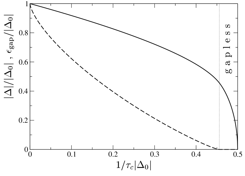
Figure 4: The order parameter $|\Delta|/|\Delta_{0}|$ (solid line) and energy gap $\epsilon_{\text{gap}}/|\Delta_{0}|$ (dashed line) versus the strength of disorder $1/\tau_{c}|\Delta_{0}|$. Here, $|\Delta_{0}|$ represents the value of the order parameter in absence of disorder. The critical value at which the order parameter disappear is given by $1/\tau_{c}|\Delta_{0}|=1/2$, while the gapless region starts at $1/\tau_{c}|\Delta_{0}|=e^{-\pi/4}\simeq 0.46$ (or equivalently at $\zeta=1/\tau_{c}|\Delta|=1$).

The mean-field equations (14) and (15) can be solved simultaneously with the mean-field Ansatz that the two order parameters are space and time independent (i.e., $\Sigma({\mathbf{r}},\tau)=\Sigma$ and $\psi_{\omega_{h},{\mathbf{p}}}=\psi\delta_{\omega_{h},0}\delta_{{\mathbf{p}},0}$), and the matrix field $Q({\mathbf{r}})$ is homogeneous in space and diagonal in the Matsubara indices. Now, through the transformation $Q\mapsto e^{i\chi\sigma_{3}/2}Qe^{-i\chi\sigma_{3}/2}$, the (homogeneous) global phase $\chi$ of the composite order parameter $\Delta$ can be gauged out of the action (13) and the equation of motion (14) can be solved, giving

$$\bar{Q}=\displaystyle\frac{u}{\sqrt{1+u^{2}}}\;\sigma_{3}\sigma_{3}^{\text{\sc{cc}}}-\displaystyle\frac{1}{\sqrt{1+u^{2}}}\;\sigma_{2}\;,$$

where the variable $u$ satisfies the equation abrikosov_gorkov :

$$\frac{\epsilon_{n}}{|\Delta|}=u-\displaystyle\frac{1}{|\Delta|\tau_{c}}\displaystyle\frac{u}{\sqrt{1+u^{2}}}\;.$$ (16)

As expected, in the mean-field approximation, the solution of the quasi-classical equations of motion become insensitive to the symmetry preserving disorder potential (i.e. the solution is independent of the classical diffusion constant $D$). Such independence is a manifestation of the Anderson theorem that protects the integrity of the condensate to impurities which do not lift the particle-hole symmetry of the system.

In the homogeneous case, the self-consistency equations for the order parameters (15) require the phases of the excitonic order parameter $\Sigma$ and of the photonic field $\psi$ to coincide, so that $|\Delta|=|\Sigma|+g|\psi|$ and from which follows the constraint:

$$\frac{1}{g}(\omega_{c}-\mu)|\psi|=\displaystyle\frac{1}{g_{c}}|\Sigma|\;.$$ (17)

Indeed, the same restriction has been found in Refs. paul ; marzena in the context of the Dicke model for the localised exciton-photon system. While the chemical potential $\mu$ does not exceed the cavity mode edge $\omega_{c}$, an order parameter $|\Delta|\neq 0$ is developed, to which both photons and the coherent polarisation contribute. Once cast in terms of the effective order parameter $\Delta$, the remaining saddle-point or mean-field equations assume the canonical form first reported by Abrikosov and Gor’kov in the context of the symmetry broken disordered superconductor abrikosov_gorkov , and later, in the present context, applied to the symmetry broken exciton insulator zittartz . To make this correspondence explicit, one may define the composite order parameter through, say, the photon condensate fraction, and an effective coupling constant as

$$|\Delta| =\left[1+\displaystyle\frac{g_{c}}{g^{2}}(\omega_{c}-\mu)\right]g|\psi|$$

$$g_{\text{eff}} =g_{c}+\displaystyle\frac{g^{2}}{\omega_{c}-\mu}\;,$$

after which the self-consistency equation reads

$$\frac{|\Delta|}{g_{\text{eff}}\nu L^{2}}=\displaystyle\frac{\pi}{\beta}\sum_{\epsilon_{n}}\displaystyle\frac{1}{\sqrt{1+u^{2}}}\;.$$ (18)

In the absence of symmetry-breaking disorder, $u=\epsilon_{n}/|\Delta|$ and the self-consistency equation coincides with the ‘gap equation’ for a bulk BCS superconductor. Keeping this analogy, convergence of the Matsubara summation demands the inclusion of an energy cut-off $E_{c}$ associated with the contact Coulomb interaction, analogous to the Debye frequency scale in the superconductor, which sets the overall scale of the order parameter. In the present case, the momentum exchange associated with the Coulomb interaction is limited by the screening length $\kappa$. As a result, the contact interaction, and therefore, the Matsubara summation, must be cut-off at the energy scale

$$E_{c}=\displaystyle\frac{p_{F}\kappa}{m}=\displaystyle\frac{p_{F}}{ma_{0}}\;.$$ (19)

In the high excitation limit where the photon coupling dominates, the cutoff should be substituted with $\varepsilon_{F}$, the overall bandwidth for electron-hole pairs.

At zero temperature, an explicit solution of the gap equation reveals the gradual suppression of the condensate as a function of the disorder strength $1/\tau_{c}|\Delta_{0}|$, leading to a complete suppression of the order parameter when $2/\tau_{c}=|\Delta_{0}|$, where $|\Delta_{0}|$ denotes the order parameter in the unperturbed system (see Fig. 4). (For a general review in the context of the symmetry broken superconductors, see, e.g., Ref. maki .) As with the disordered superconductor, the quasi-particle energy gap goes to zero faster than the order parameter, exposing a gapless phase when $2/\tau_{c}>e^{-\pi/4}|\Delta_{0}|$ or equivalently when the dimensionless parameter $\zeta\equiv 1/\tau_{c}|\Delta|$ exceeds unity. To understand how the phase behaviour of the Abrikosov-Gor’kov equations translate to the polariton system, it is necessary to explore the dependence of the chemical potential on the number of excitations.

III.1 Chemical Potential and Number of Excitations

Hitherto, we have absorbed the chemical potential into the definition of an effective Fermi energy, $\varepsilon_{F}=(\mu-E_{g})/2$, assuming this to be the largest energy scale in the problem. However, the chemical potential $\mu$ is itself fixed by the total number of excitations in the system (5). In the following, we will use this condition to explore the parameter range of validity of the approximations used to construct the theory, and to investigate the phase diagram, treating $N_{\text{ex}}$ and the symmetry breaking disorder potential $1/\tau_{c}$ as independent variables.

The validity of the model, and therefore of the self-consistency equation (18), is restricted by the hierarchy of energy scales contained in Eq. (12). Moreover, as implied by Eq. (19) above, the energy cut-off of the Coulomb interaction is, itself, dependent on the chemical potential according to the relation $E_{c}=\sqrt{\operatorname{\mathcal{R}y}(\mu-E_{g})}$, where $\operatorname{\mathcal{R}y}$ is the Rydberg energy of the electron-hole system. Taken together, the validity of the mean-field theory requires $\varepsilon_{F}=(\mu-E_{g})/2>E_{c}$ (i.e. $(\mu-E_{g})/\operatorname{\mathcal{R}y}>4$), while to stay in the weak coupling limit, we must have $E_{c}\gg|\Delta|$. In this limit, at zero temperature, the total number of excitations $N_{\text{ex}}$, which is proportional to the partial derivative of the free energy respect to the chemical potential, can be expressed in terms of the chemical potential as it follows:

$$N_{\text{ex}}=\displaystyle\frac{g^{2}}{[g_{c}(\omega_{c}-\mu)+g^{2}]^{2}}|\Delta|^{2}+\nu L^{2}\displaystyle\frac{\mu-E_{g}}{2}\;.$$

The first term describes the total number of photons $\mathcal{N}_{\text{ph}}=|\psi|^{2}$, while the second represents the total number of particle-hole excitations in the system, $\mathcal{N}_{\text{el}}=\nu L^{2}\varepsilon_{F}$. Here we have neglected terms of order $O(|\Delta|/\varepsilon_{F})$ associated with the rearrangement of states close to the Fermi energy due to the formation of the condensate. Taking into account the non-algebraic dependence of the order parameter as well as the coupling constant $g_{c}$ on $\mu$, the variation of the chemical potential with $N_{\text{ex}}$ can be inferred only numerically.

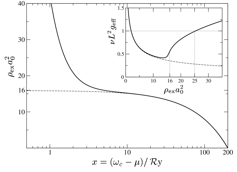
Figure 5: Normalised density of excitations $\rho_{\text{ex}}a_{0}^{2}$ as a function of the rescaled chemical potential $x=(\omega_{c}-\mu)/\operatorname{\mathcal{R}y}$ (in logarithmic scale) for $d=(\omega_{c}-E_{g})/\operatorname{\mathcal{R}y}=200$, $\tilde{g}=1$, $\lambda_{c}=10$ (bold line) and for $\tilde{g}=0$ (dashed line). The value of the density at $x=0$ for $\tilde{g}=0$, $d/4\pi\simeq 16$, has been marked. In this limit, all excitations appear as electrons and holes, allowing the population of states with energies in excess of $\omega_{c}$. The dependence from of the dimensionless effective coupling constant $\nu L^{2}g_{\text{eff}}$ on $\rho_{\text{ex}}a_{0}^{2}$ in both cases is shown in the inset. Note that the weak coupling limit imposes the constraint $\rho_{\text{ex}}a_{0}^{2}<25$.

For simplicity, let us first consider the case of a clean quantum well, $1/\tau_{c}=0$. In this case, a solution of the zero temperature self-consistency equation in the limit $\varepsilon_{F}>E_{c}\gg|\Delta_{0}|$ obtains the BCS solution

$$|\Delta_{0}|=\displaystyle\frac{E_{c}}{\sinh\left(1/\nu L^{2}g_{\text{eff}}\right)}\;.$$

Staying within the weak coupling regime, $\nu L^{2}g_{\text{eff}}<1$, to check that the system remains in the high density phase, let us recall that the Coulomb coupling constant is a function of the chemical potential (see Eq. (3)). It is convenient to introduce the dimensionless coupling constants (6). With these definitions, the total density of excitations $\rho_{\text{ex}}a_{0}^{2}=N_{\text{ex}}/L^{2}a_{0}^{2}$, takes the form

$$\rho_{\text{ex}}a_{0}^{2}\equiv\rho_{\text{el}}a_{0}^{2}+\rho_{\text{ph}}a_{0}^{2}=\displaystyle\frac{d-x}{2\pi}\left\{\displaystyle\frac{1}{2}+\right.\\ \left.+\displaystyle\frac{\tilde{g}^{2}}{(\tilde{g}^{2}+x\tilde{g}_{c}(x))^{2}}\left[\sinh\left(\displaystyle\frac{x}{\tilde{g}^{2}+x\tilde{g}_{c}(x)}\right)\right]^{-2}\right\}\;,$$ (20)

where $\rho_{\text{ph}}=\mathcal{N}_{\text{ph}}/L^{2}$ denotes the photon density and $\rho_{\text{el}}=\mathcal{N}_{\text{el}}/L^{2}\equiv 1/r_{s}^{2}$ denotes the total electron-hole density (and from which one can infer the $r_{s}$ value of the electron-hole system). Inverted, Eq. (20) describes the variation of the chemical potential (through $x$) as a function of the material parameters $\tilde{g}$, $\lambda_{c}$, $d$ and the exciton density $\rho_{\text{ex}}$.

In figure 5, the (normalised) density of excitations $\rho_{\text{ex}}a_{0}^{2}$ is plotted against the renormalised chemical potential $x$. When the density is low, the vast majority of excitations are invested in particle-hole excitations and the chemical potential scales linearly with the density, reflecting the constant density of states in the quasi two-dimensional system. As the density grows, the chemical potential $\mu$ converges on the photon band edge $\omega_{c}$, i.e. the variable $x$ diminishes to zero. Here, close to the resonance, the excitations become increasingly photon-like and $\rho_{\text{ex}}a_{0}^{2}$ diverges exponentially. The maximum density of electron-hole excitations which can be added at $\mu=\omega_{c}$ in the absence of the photon interaction, $\tilde{g}=0$, is given by $d/4\pi$. This value plays an important role, since, it represents the value of the density at which the condensate becomes dominated by photons. In fact, although both photons and electrons contribute to the formation of the condensate (i.e. to $|\Delta_{0}|$), the electronic contribution is dominant at low densities, while the screening of the Coulomb interaction results in the growth of the photon contribution at large densities. Such behaviour is illustrated most clearly in the inset of Fig. 5 where the effective coupling constant $\nu L^{2}g_{\text{eff}}$ is plotted against $\rho_{\text{ex}}a_{0}^{2}$. Increasing the density of excitations above $d/4\pi$, the effective coupling constant abruptly starts to increase until one eventually reaches the strong coupling regime where the validity of the microscopic Hamiltonian becomes uncertain. These characteristics are reflected in figure 2, where the fraction of total electrons $\rho_{\text{el}}/\rho_{\text{ex}}$ and photons $\rho_{\text{ph}}/\rho_{\text{ex}}$ are plotted as a function of the density of excitations. Moreover, making use of the equality (17), the inset shows the variation of the fraction of photons to excitons in the condensate,

$$\frac{\sqrt{\rho_{\text{ph}}a_{0}^{2}}}{N_{|\Sigma|}}=\displaystyle\frac{\tilde{g}}{\tilde{g}_{c}}\displaystyle\frac{\sqrt{4\pi}}{x}\;,$$ (21)

where $N_{|\Sigma|}=|\Sigma|\nu a_{0}^{2}$. Note that this ratio starts to deviate from zero as soon as particles are added to the system. In other words, even if small, there is a contribution from the photons to the condensate at ‘low densities’, when $\rho_{\text{ex}}a_{0}^{2}\ll d/4\pi$. Moreover, as already noted in the introduction, the increase of this quantity with the increase of the total density of excitations is due, on one hand, to the increase of the photon content as one approaches the resonance while, on the other hand, is related to the gradual decrease of Coulomb interaction and increase of the exciton-photon interaction.

So far we have focused on the character of the polariton condensate. In the next section, staying at the mean-field level, we will explore its integrity when effected by the symmetry-breaking disorder potential. Note that we have chosen particular values for the parameters $d$, $\lambda_{c}$ and $\tilde{g}$ in such a way as to expose a weak coupling regime in the high density limit. Changing their values, the main characteristics of the phase diagram remain valid, but the specific numbers can be varied. In particular, changing $d$, the regions where electron-like (lower density) or photon-like (higher density) excitations are dominant can be enlarged or reduced in size. The range of the condensed region for $\rho_{\text{ex}}a_{0}^{2}<d/4\pi$ can be varied through $\lambda_{c}$, while changes in $\tilde{g}$ characterise, when $\rho_{\text{ex}}a_{0}^{2}>d/4\pi$, variations in the gapless region and changes in the value at which the strong coupling regime is entered.

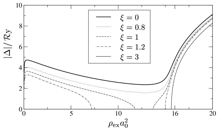
Figure 6: Order parameter $|\Delta|/\operatorname{\mathcal{R}y}$ versus $\rho_{\text{ex}}a_{0}^{2}S$ for $\tilde{g}=1$, $\lambda_{c}=10$ and $d=200$ and different values of the disorder strength $\xi=1/\tau_{c}\operatorname{\mathcal{R}y}$.

III.2 Phase Diagram

In the symmetry broken disordered system, the photon density (as recorded in the magnitude of the order parameter) has to be rescaled by the weight $|\Delta|/|\Delta_{0}|$. Fig. 4 shows the variation of the order parameter against the disorder strength $1/\tau_{c}|\Delta_{0}|$. Taking into account the dependence of the unperturbed order parameter $|\Delta_{0}|$ on the chemical potential (and therefore on the number of excitations), $|\Delta|/\operatorname{\mathcal{R}y}$ is plotted in figure 6 against $\rho_{\text{ex}}a_{0}^{2}$ for different values of $\xi=1/\tau_{c}\operatorname{\mathcal{R}y}$.

Let us consider first the dependence of the order parameter on the excitation density in the clean case: Starting from $\rho_{\text{ex}}a_{0}^{2}\gtrsim 1$, $|\Delta_{0}|$ first slightly decreases, due to the switching off of the Coulomb interaction, and then starts to increase rapidly as

$$|\Delta_{0}|/\operatorname{\mathcal{R}y}\simeq\sqrt{2\pi}\tilde{g}\sqrt{\rho_{\text{ex}}a_{0}^{2}}\;,$$ (22)

for $\rho_{\text{ex}}a_{0}^{2}>d/4\pi$. At these high values of the density, the excitations in the condensate are mainly photon-like. Therefore, increasing the disorder strength, it is not surprising that the profile of the order parameter changes little. In can be shown analytically that, in this limit, the condition $1/\tau_{c}|\Delta_{0}|>1/2$ cannot be reached. At lower densities, however, where the excitations are mainly electron-hole like, the order parameter starts to close until, increasing the value of disorder, it eventually vanishes everywhere. This behaviour is more evident from the shape of the phase diagram (see Fig. 3): In the region of density where the excitations are mainly electron-hole like, the condensed phase gets reduced, while, when the photon content starts to dominate, the condensed region expands until eventually, when $\rho_{\text{ex}}a_{0}^{2}\simeq d/4\pi$, the disorder becomes ineffective, and the line separating the two phases becomes asymptotically straight.

Analogously, one can evaluate the density and disorder dependence of the energy gap

$$\epsilon_{\text{gap}}=|\Delta|\left(1-\zeta^{2/3}\right)^{3/2}$$

and determine the region where the excitation spectrum becomes gapless, $\epsilon_{\text{gap}}=0$ (which can be equivalently established from the condition $\zeta=1/\tau_{c}|\Delta|\geq 1$). As a result, in the region dominated by the electronic excitations the gapless phase is very small and lies just below the non-condensed phase, while, when $\rho_{\text{ex}}a_{0}^{2}>d/4\pi$, the line which separates the condensed gapless region from the gapped one grows approximatively as $\sqrt{2\pi}\tilde{g}\sqrt{\rho}$.

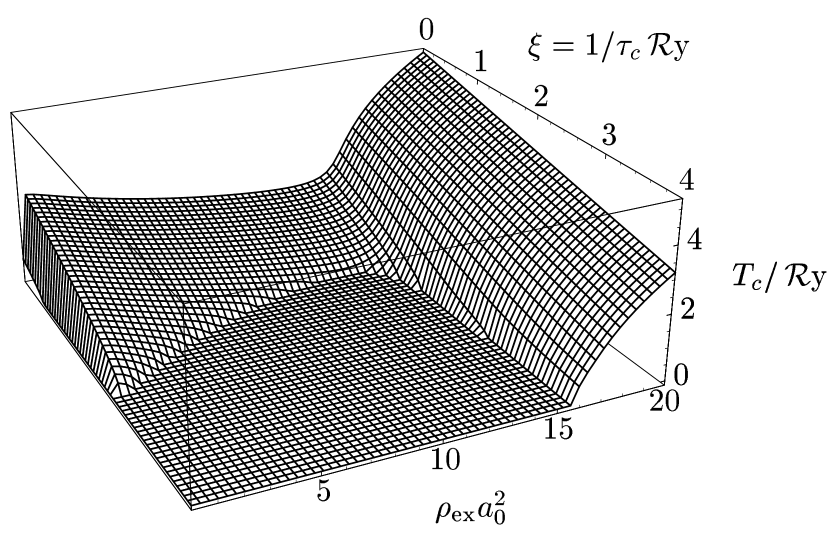
Figure 7: Three-dimensional plot of the critical temperature, $T_{c}/\operatorname{\mathcal{R}y}$, versus the disorder strength, $\xi=1/\tau_{c}\operatorname{\mathcal{R}y}$, and the excitation density, $\rho_{\text{ex}}a_{0}^{2}$ ($\tilde{g}=1$, $\lambda_{c}=10$ and $d=200$). The contour line where the critical temperature goes to zero separates the zero-temperature condensed phase from the non-condensed one and it coincides with the contour given in figure 3.

III.3 Finite Temperature

Although a rigorous treatment of the finite temperature mean-field theory would require an analysis of the thermal population of the photon degrees of freedom, one can gain a qualitative insight by approximating the chemical potential by its $T=0$ value. In this case, the variation of the critical temperature $T_{c}$ with disorder can be inferred from the gap equation through the relation abrikosov_gorkov ; maki

$$\ln\left(\displaystyle\frac{T_{c}}{T_{c0}}\right)=\psi\left(\displaystyle\frac{1}{2}\right)-\psi\left(\displaystyle\frac{1}{2}+\displaystyle\frac{1}{2\pi\tau_{c}T_{c}}\right)\;,$$

where $T_{c0}=|\Delta_{0}|e^{\gamma}/\pi$, with $\gamma\simeq 0.577$, is the critical temperature of the clean system, and $\psi(z)=\Gamma^{\prime}(z)/\Gamma(z)$ is the di-gamma function. Again, considering explicitly the dependence of the bare order parameter $|\Delta_{0}|$ on the density of excitations, it is possible to plot $T_{c}/\operatorname{\mathcal{R}y}$ as a function of both the density $\rho_{\text{ex}}a_{0}^{2}$ and disorder $\xi=1/\tau_{c}\operatorname{\mathcal{R}y}$ (see Fig. 7). The dependence of the critical temperature on the density at given values of the disorder closely mimics that of the order parameter $|\Delta|/\operatorname{\mathcal{R}y}$ given in Fig. 6: Starting from values of the densities $\rho_{\text{ex}}a_{0}^{2}\gtrsim 1$ the critical temperature starts to decrease as the Coulomb interaction weakens. When the density is high enough that the photon-like excitations are dominant, the critical temperature increases again and becomes insensitive to disorder.

This concludes our discussion of the mean-field content of the theory. In the following section, in order to explore the spectrum of excitations above the condensate, we will develop an expansion of the low-energy action in fluctuations around the mean-field.

IV Collective Excitations

In order to address important physical characteristics of the condensed polariton system we need to go beyond the mean field approximation and discuss excitation spectra. The excitations are visible through optical absorption and photoluminescence, which can provide important evidence for condensation in real systems. The phase stiffness of the condensate is another important parameter, which determines the transition temperature in the dilute limit - and in two-dimensional systems at all densities. In 2D, since there is no long range order (though there will be a Berezinskii-Kosterlitz-Thouless transition), the velocity of the Bogoliubov collective mode will determine the characteristic temperature scale at which a finite droplet of condensate can emit coherent light keeling .

Thus in this section we will explore the impact of fluctuations and how they translate to collective phenomena. The latter can be divided into separate contributions. In the first place, the system is susceptible to both spatial and temporal fluctuations of the order parameters, $|\Sigma|$ and $|\psi|$. In addition, there exist fluctuations of the matrix fields $Q({\mathbf{r}})$ which encode the influence of mechanisms of quantum interference on the excitonic degrees of freedom, the electrons and holes. In the following, we will consider an approximation engaging the rearrangement of the quasi-particle degrees of freedom in the condensate due to fluctuations of the order parameter at the saddle-point level. The impact of mesoscopic fluctuations and weak localisation phenomena on the quasi-particle excitations is left as a subject for further investigation. Drawing on the analogy with the superconducting system, we note that related calculations of the pair susceptibility have been performed in Ref. eckern_pelzer in the context of the disordered superconducting film and, more directly, in Ref. smith_ambegaokar in the context of a superconductor with magnetic impurities.

In section I.2 it was noted that the single particle Hamiltonian (10) can be expressed in terms of the single complex composite order parameter $\Delta=\Sigma+g\psi$. As such, in considering fluctuations of the total action, it is convenient to introduce a second independent field $\Gamma=\Sigma-g\psi$ and express the fluctuations of the excitonic and photonic order parameters in terms of the fluctuations of $\Delta$ and $\Gamma$, viz.

$$\begin{split}\Delta({\mathbf{r}},\tau)&=|\Delta|+\delta\Delta^{\text{\sc{l}}}({\mathbf{r}},\tau)+i\delta\Delta^{\text{\sc{t}}}({\mathbf{r}},\tau)\\ \Gamma({\mathbf{r}},\tau)&=|\Gamma|+\delta\Gamma^{\text{\sc{l}}}({\mathbf{r}},\tau)+i\delta\Gamma^{\text{\sc{t}}}({\mathbf{r}},\tau)\;,\end{split}$$ (23)

where $|\Delta|$ and $|\Gamma|$ denote the mean-field expectation values. Remembering that, at the mean-field level, the phases of $\Sigma$ and $\psi$ are locked (see Eq. (15)), one can set $|\Delta|=|\Sigma|+g|\psi|$ and $|\Gamma|=|\Sigma|-g|\psi|$, while $|\Sigma|$ and $|\psi|$ are constrained by the relation (17). In Eq. (23), longitudinal (l) and transverse (t) fluctuations represent respectively fluctuations of the amplitude and of the phase. Since our model is invariant under a global gauge transformation of the phase (11), we can anticipate that the spectrum of fluctuations will exhibit one massless Goldstone mode and three massive ones. To develop a theory for fluctuations of the condensed field $\Delta$, two of the three massive fluctuations associated with the field $\Gamma$ will be integrated out.

Fluctuations of the order parameters $\Delta$ and $\Gamma$ are not divorced from fluctuations of the fields $Q$. Indeed, through the coupling, one can expect the fluctuations of the order parameter to acquire a diffusive nature in the disordered system. Moreover, in the gapless phase, the existence of magnetic impurities should induce a mechanism of dissipation. To capture these effects, one must determine the rearrangement of the field (or self-energy) $Q$ due to fluctuations of the order parameter.

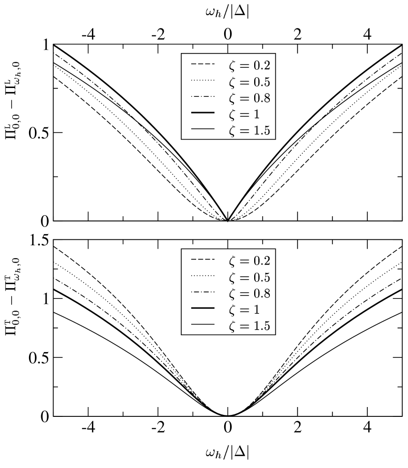
Figure 8: Zero temperature plot of the zero momentum longitudinal $\Pi_{0,0}^{\text{\sc{l}}}-\Pi_{\omega_{h},0}^{\text{\sc{l}}}$ and transverse $\Pi_{0,0}^{\text{\sc{t}}}-\Pi_{\omega_{h},0}^{\text{\sc{t}}}$ components versus the rescaled frequency $\omega_{h}/|\Delta|$, for different values of the disorder strength $\zeta=1/\tau_{c}|\Delta|$.

Denoting the homogeneous saddle-point solution associated with the mean-field as $\bar{Q}$, let us represent the rearrangement due to fluctuations as

$$Q({\mathbf{r}})=e^{W({\mathbf{r}})/2}\bar{Q}e^{-W({\mathbf{r}})/2}\;,$$ (24)

where the generators obey the symmetry relation $\{\bar{Q},W({\mathbf{r}}\}=0$. Although the calculation of the rotation $W$ in linear response is straightforward, the technical details are involved and not illuminating. As such, they have been included as an appendix. Here, we note only that, at the level of the linear response, the longitudinal and transverse components of the order parameter fluctuations do not get mixed by the $Q$-matrix action. By contrast, expanding $S_{\text{ph}}+S_{\Sigma}$ up to second order in $\delta\Delta^{\text{\sc{l,t}}}$ and $\delta\Gamma^{\text{\sc{l,t}}}$, the (massive) fluctuations of the latter can be integrated out revealing a contribution which mixes the longitudinal and transverse response. Gathering all of the contributions together, the total action takes the form

$$S_{\text{tot}}=S^{\text{\sc{ag}}}[|\Delta|,g_{\text{eff}}]+\delta S_{\text{tot}}\;,$$

where $S^{\text{\sc{ag}}}[|\Delta|,g_{\text{eff}}]$ represents the mean-field Abrikosov and Gor’kov action for a superconductor with magnetic impurities (36) and $\delta S_{\text{tot}}$ has the quadratic form

$$\frac{\delta S_{\text{tot}}}{\beta\nu L^{2}}=\sum_{\omega_{h},{\mathbf{p}}}\begin{pmatrix}\delta\Delta^{\text{\sc{l}}}\\ \delta\Delta^{\text{\sc{t}}}\end{pmatrix}^{\mathsf{T}}_{-\omega_{h},-{\mathbf{p}}}G^{-1}_{\omega_{h},{\mathbf{p}}}\begin{pmatrix}\delta\Delta^{\text{\sc{l}}}\\ \delta\Delta^{\text{\sc{t}}}\end{pmatrix}_{\omega_{h},{\mathbf{p}}}\;.$$ (25)

Here the kernel $G^{-1}_{\omega_{h},{\mathbf{p}}}$ denotes the inverse of the thermal Green’s function or susceptibility:

$$G^{-1}_{\omega_{h},{\mathbf{p}}}=\begin{pmatrix}-\Pi^{\text{\sc{l}}}_{\omega_{h},{\mathbf{p}}}+\Theta_{\omega_{h},{\mathbf{p}}}&\Lambda_{-\omega_{h},{\mathbf{p}}}\\ \Lambda_{\omega_{h},{\mathbf{p}}}&-\Pi^{\text{\sc{t}}}_{\omega_{h},{\mathbf{p}}}+\Theta_{\omega_{h},{\mathbf{p}}}\end{pmatrix}\;.$$ (26)

We refer to appendix A for details and the explicit expressions of the Green’s function elements. Let us note here that, if we restrict attention to the condensate phase $|\Delta|\neq 0$, the self-consistency equation (18) translates to the condition

$$\Theta_{0,0}\equiv\displaystyle\frac{1}{\nu L^{2}g_{\text{eff}}}=\Pi^{\text{\sc{t}}}_{0,0}\;,$$ (27)

rendering the transverse fluctuations of the quasi-particle degrees of freedom massless. By contrast, when $|\Delta|=0$, the longitudinal and transverse kernels coincide, $\Pi^{\text{\sc{l}}}_{\omega_{h},{\mathbf{p}}}=\Pi^{\text{\sc{t}}}_{\omega_{h},{\mathbf{p}}}$ and acquire a mass, which, at zero temperature, is given by

$$\Theta_{0,0}-\Pi^{\text{\sc{l,t}}}_{0,0}=\ln\left(\displaystyle\frac{2}{|\Delta_{0}|\tau_{c}}\right)\;.$$

As expected from the mean-field analysis, when $2/|\Delta_{0}|\tau_{c}=1$ the mass disappears and the system undergoes a transition to a condensate phase.

The form in Eq. (25) is positive definite, determining the stability of the mean-field solution against fluctuations. Moreover it is already clear from the form of the kernel (26) and from the constraint (27) that the excitation spectra of the system admits a massless Goldstone mode and a massive one. In fact, considering the zero frequency and zero momentum component, the anti-diagonal term $\Lambda_{0,0}$ vanishes together with the transverse one, $(G^{-1}_{0,0})_{22}$, while the longitudinal component $(G^{-1}_{0,0})_{11}$ remains finite.

In fact, the precise functional forms $\Pi^{\text{\sc{l,t}}}_{\omega_{h},{\mathbf{p}}}$ coincide with those found for a disordered superconductor in the presence of magnetic impurities smith_ambegaokar . Their frequency dependence is plotted in figure 8: With $\Pi_{\omega_{h},0}^{\text{\sc{t}}}$, no qualitative change is associated with the transition to the gapless region for $\zeta\geq 1$; the quadratic character of the dispersion at small frequencies is preserved. By contrast, as the system enters the gapless phase $\zeta\geq 1$, with the longitudinal component $\Pi_{\omega_{h},0}^{\text{\sc{l}}}$ exhibits a dissipative dependence scaling linearly with frequency.

In order to elucidate this behaviour further, it is convenient to affect a gradient expansion of the kernel (26), whereupon, at zero temperature, one finds

$$G^{-1}_{\omega_{h},{\mathbf{p}}}\simeq\begin{pmatrix}c_{1}+\displaystyle\frac{1}{2}a_{1}\displaystyle\frac{D{\mathbf{p}}^{2}}{|\Delta|}+\displaystyle\frac{1}{2\zeta}\displaystyle\frac{|\omega_{h}|}{|\Delta|}\theta(\zeta-1)+\displaystyle\frac{1}{2}b_{1}\left(\displaystyle\frac{\omega_{h}}{|\Delta|}\right)^{2}&-f\displaystyle\frac{\omega_{h}}{|\Delta|}\\ f\displaystyle\frac{\omega_{h}}{|\Delta|}&\displaystyle\frac{1}{2}a_{2}\displaystyle\frac{D{\mathbf{p}}^{2}}{|\Delta|}+\displaystyle\frac{1}{2}b_{2}\left(\displaystyle\frac{\omega_{h}}{|\Delta|}\right)^{2}\end{pmatrix}\;,$$ (28)

with

$$a_{1} =a_{\text{\sc{l}}}(\zeta)+a a_{2} =a_{\text{\sc{t}}}(\zeta)+a$$

$$b_{1} =b_{\text{\sc{l}}}(\zeta)+b b_{2} =\frac{1}{2}+b\;.$$ (29)

The coefficients $c_{1}=c_{\text{\sc{l}}}(\zeta)$, $a_{\text{\sc{l,t}}}(\zeta)$ and $b_{\text{\sc{l,t}}}(\zeta)$ derive from the expansion of the kernels $\Pi^{\text{\sc{l,t}}}_{\omega_{h},{\mathbf{p}}}$ moir . Although the explicit expression for their dependency on the disorder strength $\zeta$ can be rigorously derived (or equivalently can be numerically inferred from figure (8)), we note here that, as soon as $|\Delta|\neq 0$, these parameters are of $O(1)$ and in particular, at zero disorder strength $\zeta=0$, they are given by $c_{\text{\sc{l}}}(0)=1$, $a_{\text{\sc{l}}}(0)=\pi/4$, $a_{\text{\sc{t}}}(0)=\pi/2$, $b_{\text{\sc{l}}}(0)=1/6$. More significantly, in the gapless region $\zeta>1$, the longitudinal kernel acquires a dissipative term and the coefficient $b_{\text{\sc{l}}}(\zeta)$ changes of sign and becomes negative. In contrast, making use of the dimensionless parameters introduced in Eq. (6), the expansion of the kernels $\Theta_{\omega_{h},{\mathbf{p}}}$ and $\Lambda_{\omega_{h},{\mathbf{p}}}$, gives

$$a =\displaystyle\frac{\tilde{g}^{2}}{[\tilde{g}^{2}+\tilde{g}_{c}(x)x]^{2}}\displaystyle\frac{c^{2}}{D\omega_{c}}\left(\displaystyle\frac{|\Delta|}{\operatorname{\mathcal{R}y}}\right)$$

$$b =\displaystyle\frac{2\tilde{g}^{2}\tilde{g}_{c}(x)}{[\tilde{g}^{2}+\tilde{g}_{c}(x)x]^{3}}\left(\displaystyle\frac{|\Delta|}{\operatorname{\mathcal{R}y}}\right)^{2}$$

$$f =\displaystyle\frac{\tilde{g}^{2}}{[\tilde{g}^{2}+\tilde{g}_{c}(x)x]^{2}}\left(\displaystyle\frac{|\Delta|}{\operatorname{\mathcal{R}y}}\right)\;.$$

IV.1 Gapped Phase

The spectrum of the collective excitations is determined by the poles of the matrix $G_{\omega_{h},{\mathbf{p}}}$ and therefore by the zeros of the expression $\det(G^{-1}_{\omega_{h},{\mathbf{p}}})$. Let us consider first the gapped phase, $\zeta<1$, where the determinant of the kernel can be evaluated exactly:

$$\det\left(G^{-1}_{\omega_{h},{\mathbf{p}}}\right)=\left(\displaystyle\frac{\omega_{h}^{2}}{|\Delta|^{2}}+\displaystyle\frac{E_{1}^{2}}{|\Delta|^{2}}\right)\left(\displaystyle\frac{\omega_{h}^{2}}{|\Delta|^{2}}+\displaystyle\frac{E_{2}^{2}}{|\Delta|^{2}}\right)\;.$$

The energies $E_{1,2}$, which can be shown for each value of the momentum to be real, are plotted in figure 9. From this we can infer that the spectrum of excitations, which is obtained by analytically continuing to real energies (i.e., substituting $\omega_{h}\mapsto i\varepsilon$), is given by a linear (massless) branch and a quadratic (massive) branch, where, expanding for small values of momentum, the gap of the massive mode and the ‘velocity’ associated with the massless mode are respectively given by:

$$\displaystyle\frac{E_{1}}{|\Delta|} \operatorname*{\simeq}_{{\mathbf{p}}\to 0}\sqrt{\displaystyle\frac{2b_{2}c_{1}+4f^{2}}{b_{1}b_{2}}}$$

$$\displaystyle\frac{E_{2}}{|\Delta|} \operatorname*{\simeq}_{{\mathbf{p}}\to 0}\sqrt{\displaystyle\frac{a_{2}c_{1}}{b_{2}c_{1}+2f^{2}}}\sqrt{\displaystyle\frac{D{\mathbf{p}}^{2}}{|\Delta|}}\;.$$

In order to gain some physical insight into these parameters, once they are expressed in terms of the coefficients (29), two opposite limits can be identified. In the first case, when $1<\rho_{\text{ex}}a_{0}^{2}\ll d/4\pi$ (i.e. for $x\gg 1$, $\tilde{g}_{c}(x)x\gg\tilde{g}$ and $|\Delta|/\operatorname{\mathcal{R}y}<O(1)$) one expects $a_{\text{\sc{l,t}}}\gg a$ and $b_{\text{\sc{l,t}}}\gg b,f$, whereupon

$$E_{1} \operatorname*{\simeq}_{{\mathbf{p}}\to 0}\sqrt{\displaystyle\frac{2c_{\text{\sc{l}}}}{b_{\text{\sc{l}}}}}|\Delta|\operatorname*{\to}_{\zeta\to 0}2\sqrt{3}|\Delta_{0}|$$

$$E_{2} \operatorname*{\simeq}_{{\mathbf{p}}\to 0}\sqrt{\displaystyle\frac{a_{\text{\sc{t}}}}{b_{\text{\sc{t}}}}}\sqrt{D|\Delta|}|{\mathbf{p}}|\operatorname*{\to}_{\zeta\to 0}\sqrt{\pi}\sqrt{D|\Delta_{0}|}|{\mathbf{p}}|\;.$$

Therefore, in the gapped phase, for values of the density at which the excitations are largely electronic in character (see Fig. 2), the gap for the massive collective excitations is proportional to the composite order parameter $|\Delta|$, while the velocity of the massless excitations is given by the product of the coherence length $\xi_{\text{coh}}=\sqrt{D/|\Delta|}$ and the order parameter comment .

In the opposite limit, $\rho_{\text{ex}}a_{0}^{2}\gg d/4\pi$ (i.e. for $x\to 0$, and, taking into account the density dependence of the order parameter in this limit (22), for $d/4\pi>\tilde{g}^{2}/\tilde{g}_{c}(x)$), we can use the approximations $a\gg a_{\text{\sc{l,t}}}$ and $b,f\gg b_{\text{\sc{l,t}}}$, which translates to

$$E_{1} \operatorname*{\simeq}_{{\mathbf{p}}\to 0}\displaystyle\frac{\tilde{g}^{2}}{\tilde{g}_{c}(x)}\operatorname{\mathcal{R}y}$$

$$E_{2} \operatorname*{\simeq}_{{\mathbf{p}}\to 0}\tilde{g}\sqrt{\displaystyle\frac{c_{\text{\sc{l}}}}{2(\omega_{c}/\operatorname{\mathcal{R}y})(1+c_{\text{\sc{l}}})}}c{\mathbf{p}}\;.$$

When the density is so high that photons dominate, but still $g_{c}(x)\neq 0$, the gap in the collective excitation spectrum is given by the ratio of the square of the photon coupling to the Coulomb coupling constant, while the velocity is proportional to the velocity of light $c$. Note that in absence of Coulomb interaction, $g_{c}\equiv 0$, the coefficient $b$ vanishes and the situation is different: the gap is in fact proportional to $|\Delta|=g|\psi|$ in the first limit and to $|\psi|^{2}/\nu L^{2}$ in the very high density regime.

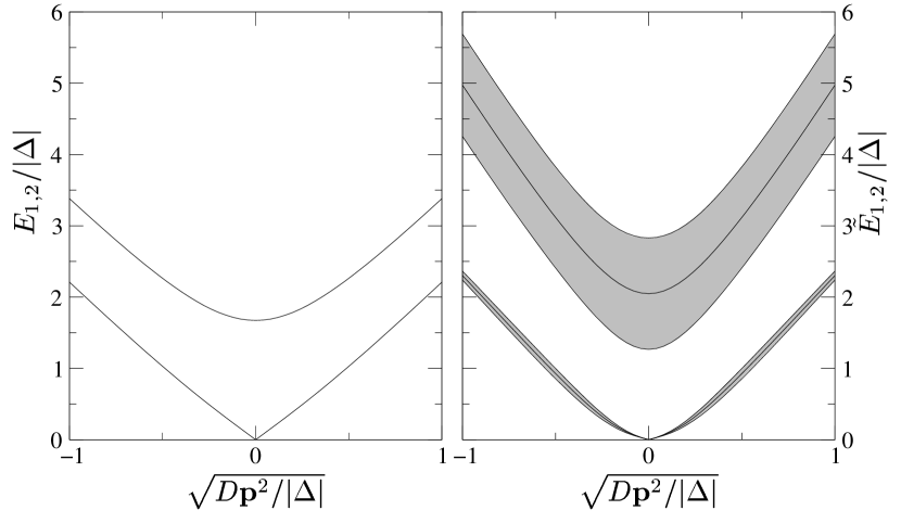
Figure 9: Dispersion of the collective excitation spectrum in the gapped $\zeta<1$ (left) and gapless $\zeta>1$ (right) regions. Here, we have chosen the particular values $c_{1}=0.8$, $a_{1}=7.1$, $a_{2}=7.7$, $b_{1}=1$, $b_{2}=1.2$ and $f=0.6$ (corresponding to $\rho_{\text{ex}}a_{0}^{2}=16$, $\xi=1/\tau_{c}\operatorname{\mathcal{R}y}=1$ and $D\omega_{c}/c^{2}=0.1$) in the first case, and $c_{1}=0.1$, $a_{1}=7.6$, $a_{2}=7.6$, $b_{1}=0.4$, $b_{2}=1.1$ and $f=0.7$ (corresponding to $\rho_{\text{ex}}a_{0}^{2}=16$, $\xi=4$ and $D\omega_{c}/c^{2}=0.1$) in the second (note that this choice masks the actual linear dispersion of the massless mode). When $\zeta>1$, both the massive and massless excitations acquire a finite life time with, respectively the first finite and almost constant, while the second exhibits a quadratic dispersion and therefore null at zero momentum. Their line widths, $\Re\tilde{E}_{1,2}\pm\Im\tilde{E}_{1,2}$, are explicitly plotted.

IV.2 Gapless Phase

Let us consider now the gapless region $\zeta>1$. In the leading approximation, one may neglect the quadratic term $b_{1}\omega_{h}^{2}/|\Delta|^{2}$, obtaining

$$\det\left(G^{-1}_{\omega_{h},{\mathbf{p}}}\right)=\left(i\displaystyle\frac{|\omega_{h}|}{|\Delta|}+\displaystyle\frac{\tilde{E}_{1}}{|\Delta|}\right)\left(-i\displaystyle\frac{|\omega_{h}|}{|\Delta|}-\displaystyle\frac{\tilde{E}_{2}}{|\Delta|}\right)$$

$$\displaystyle\frac{\tilde{E}_{1,2}}{|\Delta|}\operatorname*{\simeq}_{{\mathbf{p}}\to 0}\pm\sqrt{\displaystyle\frac{a_{2}c_{1}}{b_{2}c_{1}+2f^{2}}}\sqrt{\displaystyle\frac{D{\mathbf{p}}^{2}}{|\Delta|}}+i\displaystyle\frac{a_{2}}{4\zeta(b_{2}c_{1}+2f^{2})}\displaystyle\frac{D{\mathbf{p}}^{2}}{|\Delta|}\;.$$

Therefore, analytically continuing to real energies ($|\omega_{h}|\to i\varepsilon$), the massless modes $E_{2}$ acquires a positive imaginary part with a quadratic dispersion in terms of the momentum ${\mathbf{p}}$. In other words the massless mode has a finite life time (or line width) whenever ${\mathbf{p}}\neq 0$. In order to evaluate the life time of the massive modes $E_{1}$, one has to restore the quadratic term $b_{1}\omega_{h}^{2}/|\Delta|$. Considering for simplicity a value of the density $\rho_{\text{ex}}a_{0}^{2}$ and the disorder $\xi=1/\tau_{c}\operatorname{\mathcal{R}y}$ for which the coefficient $b_{1}$ is overall positive, the spectrum is plotted in figure 9. (Note that close to the transition between the gapped and the gapless region, the coefficient $b_{1}$ can become negative, in which case, to reestablish stability, one has to introduce the next order in frequency of the expansion.)

We finally note that, in the non-condensed region $|\Delta|=0$ (i.e., at zero temperature, for values of the disorder strength $2/\tau_{c}|\Delta_{0}|>1$), the kernel acquires a mass proportional to $\ln(2/\tau_{c}|\Delta_{0}|)$, while the massless modes disappear.

IV.3 Number of Photonic Occupied Modes

Experimentally, the spectrum of collective excitations can be accessed indirectly by measuring the angle resolved photoluminescence intensity associated with the small leakage of photons from the cavity. The latter provides a convenient way of mapping the occupation density of the photon modes,

$$\mathcal{N}_{\text{ph}}({\mathbf{p}})=\lim_{\eta\to 0^{+}}\langle\psi^{\dagger}_{{\mathbf{p}}}(\tau+\eta)\psi_{{\mathbf{p}}}(\tau)\rangle\;,$$

where the in-plane quantum well momentum is determined by the angle $\phi$ at which the light is detected, $|{\mathbf{p}}|=(\omega_{c}/c)\tan\phi$. Taken at the level of the mean-field approximation, the transition to the condensed phase would be associated with the development of a sharp coherent peak in the density distribution at ${\mathbf{p}}=0$. However, in the quasi two-dimensional quantum well geometry, the proliferation of massless phase modes destroys true long range order. Instead, the bulk transition to the condensed phase is of Berezinskii-Kosterlitz-Thouless type chaikin_lubensky . In this case, one expects the bulk transition to be reflected in the development of power-law correlations in the density distribution. Strictly speaking, to infer the characteristic power-law dependence of the correlations, one should restore gauge invariance of the action under global phase rotations. However, guided by a parallel investigation of trapped excitons in Ref. keeling , one can infer the nature of the long ranged correlations simply from the spectrum of the phase mode determined above.

In the present case the calculation is complicated slightly by the fact that, to establish the impact of the massless collective fluctuations on the photon distribution, one must find their projection onto the phase mode associated with the photon field. This, in turn, introduces a ‘form factor’ which reflects the superfluid stiffness. Then, when parameterized as $\psi({\mathbf{r}})=|\psi({\mathbf{r}})|e^{i\theta({\mathbf{r}})}$, discarding massive fluctuations, one obtains the characteristic power-law divergence footnote_fluct

$$\langle\theta_{-{\mathbf{p}}}\theta_{{\mathbf{p}}}\rangle\operatorname*{\simeq}_{{\mathbf{p}}\to 0}\displaystyle\frac{k_{\text{\sc{b}}}T}{\rho_{s}({\mathbf{p}}L)^{2}}\;,$$ (30)

with the (superfluid) stiffness given by

$$\rho_{s}=\displaystyle\frac{[\tilde{g}^{2}+\tilde{g}_{c}(x)x]^{2}}{\tilde{g}^{2}}\displaystyle\frac{a_{2}}{2}\left(\displaystyle\frac{\xi_{\text{coh}}}{L}\right)^{2}\operatorname{\mathcal{R}y}\psi^{2}\;,$$

where $\xi_{\text{coh}}=\sqrt{D/|\Delta|}$ is the superconducting coherence length. The corresponding spatial correlation function assumes the characteristic logarithmic divergence at long distances:

$$g({\mathbf{r}})\equiv\displaystyle\frac{1}{2}\langle\left[\theta({\mathbf{r}})-\theta(0)\right]^{2}\rangle\operatorname*{\simeq}_{|{\mathbf{r}}|\to\infty}\displaystyle\frac{k_{\text{\sc{b}}}T}{2\pi\rho_{s}}\ln\left(\displaystyle\frac{|{\mathbf{r}}|}{\xi_{T}}\right)\;,$$

where $\xi_{T}\propto\xi_{\text{coh}}|\Delta|/k_{\text{\sc{b}}}T$ represents the thermal length. Restoring gauge invariance, and noting that the dominant contribution to the amplitude mode comes from mean-field, we obtain:

$$\mathcal{N}_{\text{ph}}({\mathbf{p}})=|\psi|^{2}\int\displaystyle\frac{d{\mathbf{r}}}{L^{2}}e^{i{\mathbf{p}}\cdot{\mathbf{r}}-g({\mathbf{r}})}\;.$$

This integral can be exactly evaluated in two-dimensions, giving, for temperatures $\eta=k_{\text{\sc{b}}}T/2\pi\rho_{s}<2$, the result:

$$\mathcal{N}_{\text{ph}}({\mathbf{p}})=4\pi\displaystyle\frac{|\psi|^{2}}{L^{2}}\left(\displaystyle\frac{\xi_{T}}{2}\right)^{\eta}\displaystyle\frac{\Gamma(1-\eta/2)}{\Gamma(\eta/2)}\displaystyle\frac{1}{|{\mathbf{p}}|^{2-\eta}}\;.$$ (31)

As noted at the end of section IV.2, when $|\Delta|=0$, the amplitude and phase modes coincide and, in particular, the phase mode acquires a mass proportional to the distance from the critical point. Here, in the non-condensed phase, the density distribution asymptotes to a constant at small ${\mathbf{p}}$.

V Conclusions

In this paper, we have investigated the properties of a model for cavity polaritons in the high density regime, where the interplay between Coulomb interaction, the photon mediated coupling and the effect of disorder in the quantum well gives rise to different domains in the phase diagram. Changing the density, we have shown that the character of the condensate changes from being excitonic in character to photonic. The effective coupling constant is determined by the sum of the direct screened Coulomb interaction and the effective interaction induced by the exchange of photons. When the condensate has largely excitonic character, we have shown that the ‘charged’ disorder presents a pair-breaking channel which destabilises the condensate phase. Increasing the density of excitations, the system moves towards a region dominated by photons. Here, the increasing insensitivity of the condensate to disorder inhibits the complete quenching of coherence, while leaving open the possibility of a gapless region where the condensate manifests the properties of a semiconductor laser. In the condensed phase, across the whole range of densities, we have determined the spectrum of collective excitations.

The parameter regimes we have explored are in principle accessible in semiconductor microcavities. In III-V and II-VI semiconductors, microcavities have been constructed with measured values of the Rabi splitting approaching $30\text{meV}$ lesidang , and even larger values for an organic semiconductor lidzey . Since the exciton Rydberg and inverse density of states take values similar to or smaller than this energy (depending on material), the dimensionless photon coupling $\tilde{g}$ can be made of order unity. To reach the high density ‘plasma’ regime for the electron-hole system, one must obtain electron-hole densities $\rho_{\text{el}}a_{0}^{2}$ of order unity or greater, but this is indeed the typical operating density of a semiconductor laser. Indeed semiconductor lasers are conventionally modelled as a degenerate electron-hole plasma, though of course their operation is conventionally at temperatures somewhat larger than the Rydberg. Perhaps more important than their temperature is that real lasers are open systems and thus have dynamical decoherence and dephasing processes that we have not included here. To the extent that pair-breaking by static disorder mimics dynamically induced decoherence, we may interpret the pair-breaking parameter $\zeta$ as the dephasing rate $T_{2}^{-1}$ introduced into laser rate equations. With this identification parameters for a conventional laser sclaser are indeed well in the limit $\zeta\gg 1$.

As a final remark, for the clean system, the model considered in this work bears similarity with that discussed in the context of atomic condensation. The polariton Hamiltonian considered in this work has been used by many to model the atom/molecule interaction in a Fermi system positioned close to a Feshbach resonance (see, e.g., Ref. timmermans_holland_ohashi_griffin ). With an appropriate dictionary of correspondence, both the mean-field content of the theory as well as the spectrum of collective excitations can be compared in the two systems.

Appendix A Second Variation

As outlined in section IV, the second variation $\delta S_{\text{tot}}=\delta S[Q]+\delta S_{\text{ph}+\Sigma}$ of the total action is given by two contributions, one coming from the action for the semiclassical Green function (13) and the other from the photonic (8) and excitonic (9) actions. Starting with the first contribution, we consider the parameterization (24) for the $Q({\mathbf{r}})$ matrix and linearize the equation of motion (14) in the fluctuation terms $W({\mathbf{r}})$ and $\delta\Delta^{\text{\sc{l,t}}}_{\omega_{h}}({\mathbf{r}})$,

$$-D\nabla^{2}W+[\hat{\mathcal{O}},\bar{Q}W]-\displaystyle\frac{1}{2\tau_{c}}[\bar{Q},\sigma_{3}\sigma_{3}^{\text{\sc{cc}}}\bar{Q}W\sigma_{3}\sigma_{3}^{\text{\sc{cc}}}]\\ =-[\delta\Delta^{\text{\sc{l}}}\sigma_{2}+\delta\Delta^{\text{\sc{t}}}\sigma_{1},\bar{Q}]\;,$$

where the operator

$$\hat{\mathcal{O}}=\hat{\epsilon}\sigma_{3}\sigma_{3}^{\text{\sc{cc}}}-|\Delta|\sigma_{2}+\displaystyle\frac{1}{2\tau_{c}}\sigma_{3}\sigma_{3}^{\text{\sc{cc}}}\bar{Q}\sigma_{3}\sigma_{3}^{\text{\sc{cc}}}\;,$$

generates the mean-field equation of motion, $[\hat{\mathcal{O}},\bar{Q}]=0$. The equation for $W({\mathbf{r}})$ can be easily solved in term of the components $W=w_{0}\openone+{\mathbf{w}}\cdot{\boldsymbol{\sigma}}\sigma_{3}^{\text{\sc{cc}}}$. Then, this solution can be substituted back into the action (13), which expanded up to the second order, reads as $S[Q]=S[\bar{Q}]+\delta S[Q]$, where

$$\delta S[Q]=-\displaystyle\frac{\pi\nu}{8}\int d{\mathbf{r}}\operatorname{tr}\left([\delta\Delta^{\text{\sc{l}}}\sigma_{2}+\delta\Delta^{\text{\sc{t}}}\sigma_{1},\bar{Q}]W\right)\;.$$

Substituting the solutions for $w_{0}$ and ${\mathbf{w}}$, one obtains

$$\delta S[Q]=-\nu L^{2}\beta\sum_{\omega_{h},{\mathbf{p}}}\left[\delta\Delta_{-\omega_{h},-{\mathbf{p}}}^{\text{\sc{l}}}\Pi^{\text{\sc{l}}}_{\omega_{h},{\mathbf{p}}}\delta\Delta_{\omega_{h},{\mathbf{p}}}^{\text{\sc{l}}}\right.\\ \left.+\delta\Delta_{-\omega_{h},-{\mathbf{p}}}^{\text{\sc{t}}}\Pi^{\text{\sc{t}}}_{\omega_{h},{\mathbf{p}}}\delta\Delta_{\omega_{h},{\mathbf{p}}}^{\text{\sc{t}}}\right]\;,$$ (32)

where the kernels $\Pi^{\text{\sc{l,t}}}_{\omega_{h},{\mathbf{p}}}$ are given by:

$$\begin{split}\Pi^{\text{\sc{l,t}}}_{\omega_{h},{\mathbf{p}}}&=\displaystyle\frac{\pi}{\beta|\Delta|}\sum_{\epsilon_{n}}\Omega^{\text{\sc{l,t}}}_{{\mathbf{p}}}(u(\epsilon_{n}),u(\epsilon_{n}+\omega_{h}))\\ \Omega^{\text{\sc{l}},\text{\sc{t}}}_{{\mathbf{p}}}(u_{1},u_{2})&=\displaystyle\frac{1+\displaystyle\frac{u_{1}u_{2}\mp 1}{\sqrt{1+u_{1}^{2}}\sqrt{1+u_{2}^{2}}}}{\displaystyle\frac{D{\mathbf{p}}^{2}}{|\Delta|}+\sqrt{1+u_{1}^{2}}+\sqrt{1+u_{2}^{2}}-\zeta\left(1-\displaystyle\frac{u_{1}u_{2}\mp 1}{\sqrt{1+u_{1}^{2}}\sqrt{1+u_{2}^{2}}}\right)}\;,\end{split}$$ (33)

Turning to the second contribution, one has to expand $S_{\text{ph}}+S_{\Sigma}$ around the mean field value of the photon field $|\psi|$ and of excitonic order parameter $|\Sigma|$. As suggested in section IV, it is convenient to introduce a new order parameter $\Gamma({\mathbf{r}},\tau)$ and parameterise the fluctuations as in Eq. (23). Once expanded up to the second order, the variables $\delta\Gamma^{\text{\sc{l}},\text{\sc{t}}}_{\pm\omega_{h}}$ can be eliminated via a Gaussian integral. In this way, $S_{\text{ph}}+S_{\Sigma}=\beta(\omega_{c}-\mu)|\psi|^{2}+\beta|\Sigma|^{2}/g_{c}+\delta S_{\text{ph}+\Sigma}$, where

$$\delta S_{\text{ph}+\Sigma}=\beta\sum_{\omega_{h},{\mathbf{p}}}\left\{\delta\Delta^{\text{\sc{l}}}_{-\omega_{h},-{\mathbf{p}}}\Theta_{\omega_{h},{\mathbf{p}}}\delta\Delta^{\text{\sc{l}}}_{\omega_{h},{\mathbf{p}}}\right.\\ \left.+\delta\Delta^{\text{\sc{t}}}_{-\omega_{h},-{\mathbf{p}}}\Theta_{\omega_{h},{\mathbf{p}}}\delta\Delta^{\text{\sc{t}}}_{\omega_{h},{\mathbf{p}}}+\delta\Delta^{\text{\sc{l}}}_{-\omega_{h},-{\mathbf{p}}}\Lambda_{-\omega_{h},{\mathbf{p}}}\delta\Delta^{\text{\sc{t}}}_{\omega_{h},{\mathbf{p}}}\right.\\ \left.+\delta\Delta^{\text{\sc{t}}}_{-\omega_{h},-{\mathbf{p}}}\Lambda_{\omega_{h},{\mathbf{p}}}\delta\Delta^{\text{\sc{l}}}_{\omega_{h},{\mathbf{p}}}\right\}\;,$$ (34)

and the terms $\Theta_{\omega_{h},{\mathbf{p}}}$ and $\Lambda_{\omega_{h},{\mathbf{p}}}$ are respectively given by:

$$\begin{split}\Theta_{\omega_{h},{\mathbf{p}}}&=\displaystyle\frac{1}{\nu L^{2}}\displaystyle\frac{g^{2}\left[\omega({\mathbf{p}})-\mu\right]+g_{c}\left[\omega({\mathbf{p}})-\mu\right]^{2}+g_{c}\omega_{h}^{2}}{\left\{g^{2}+g_{c}\left[\omega({\mathbf{p}})-\mu\right]\right\}^{2}+g_{c}^{2}\omega_{h}^{2}}\\ \Lambda_{\omega_{h},{\mathbf{p}}}&=\displaystyle\frac{1}{\nu L^{2}}\displaystyle\frac{g^{2}\omega_{h}}{\left\{g^{2}+g_{c}\left[\omega({\mathbf{p}})-\mu\right]\right\}^{2}+g_{c}^{2}\omega_{h}^{2}}\;.\end{split}$$ (35)

Note that the the term $1/\nu L^{2}$ is here necessary since, in the thermodynamic limit, the Coulomb and photon coupling constant have to be rescaled with the volume according to the definitions (6).

Finally, the mean-field value of the total action

$$S^{\text{\sc{ag}}}[|\Delta|,g_{\text{eff}}]=\beta(\omega_{c}-\mu)|\psi|^{2}+\beta|\Sigma|^{2}/g_{c}+S[\bar{Q}]\;,$$ (36)

coincides with the Abrikosov and Gor’kov theory for a superconductor with magnetic impurities (see, e.g., maki ).

- (1) J. J. Hopfield, Phys. Rev 112, 1555 (1958).
- (2) L. V. Keldysh, “Macroscopic coherent states of excitons in semiconductors”. In Bose Einstein Condensation (Eds. Griffin, A., Snoke, D. W., and Stringari, S.), 246. Cambridge University Press, Cambridge (1995).
- (3) S. A. Moskalenko and D. W. Snoke, Bose-Einstein Condensation of Excitons and Biexcitons, Cambridge University Press, Cambridge (2000).
- (4) H. Haug and S. Koch, Quantum Theory of the Optical and Electronic Properties of Semiconductors, World Scientific (1990).
- (5) C. Weisbuch, M. Nishioka, A. Ishikawa, and Y. Arakawa, Phys. Rev. Lett. 69, 3314 (1992).
- (6) Le Si Dang, D. Heger, R. André, F. Boeuf, and R. Romestain, Phys. Rev. Lett. 81, 3920 (1998).
- (7) D. G. Lidzey, D. D. C. Bradley, M. S. Skolnick, T. Virgili, S. Walker, and D. M. Whittaker, Nature 395, 53 (1998).
- (8) P. G. Savvidis, J. J. Baumberg, R. M. Stevenson, M. S. Skolnick, D. M. Whittaker, and J. S. Roberts, Phys. Rev. Lett. 84, 1547 (2000); J. J. Baumberg, P. G. Savvidis, R. M. Stevenson, A. I. Tartakovskii, M. S. Skolnick, D. M. Whittaker, and J. S. Roberts, Phys. Rev. B 62, R16247 (2000); M. Saba, C. Ciuti, J. Bloch, V. Thierry-Mieg, R. André, Le Si Dang, S. Kundermann, A. Mura, G. Bongiovanni, J. L. Staehli, and B. Deveaud, Nature 414, 731 (2001).
- (9) R. Huang, Y. Yamamoto, R. André, J. Bleuse, M. Muller, and H. Ulmer-Tuffigo, Phys. Rev. B 65, 165314 (2002).
- (10) H. Deng, G. Weihs, C. Santori, J. Bloch, and Y. Yamamoto, Science 298, 199 (2002); H. Deng, G. Weihs, D. Snoke, J. Bloch, and Y. Yamamoto, PNAS 100, 15318 (2003).
- (11) F. Tassone, C. Piermarocchi, V. Savona, A. Quattropani, and P. Schwendimann, Phys. Rev. B 56, 7554 (1997); F. Tassone and Y. Yamamoto, Phys. Rev. B 59, 10830 (1999).
- (12) A. I. Tartakovskii, M. Emam-Ismail, R. M. Stevenson, M. S. Skolnick, V. N. Astratov, D. M. Whittaker, J. J. Baumberg, and J. S. Roberts, Phys. Rev. B 62, R2283 (2000).
- (13) See, e.g., A. Kavokin and G. Malpuech, Thin Films and Nanostructures Vol. 32, Cavity Polaritons, Academic Press, Amsterdam (2003), and reference therein; D. Porras, C. Ciuti, J. J. Baumberg, and C. Tejedor, Phys. Rev. B 66, 085304 (2002).
- (14) L. V. Keldysh and Yu. V. Kopaev, Fiz. Tverd. Tela (Leningrad) 6, 2791 (1964) [Sov. Phys. Solid State 6, 2219 (1965)]; L. V. Keldysh and A. N. Kozlov, Zh. Éksp. Teor. Fiz. 54, 978 (1968) [Sov. Phys. JETP 27, 521 (1968)].
- (15) C. Comte and P. Nozières, J. Physique 43, 1069 (1982); P. Nozières and C. Comte, J. Physique 43, 1083 (1982).
- (16) S. Schmitt-Rink and D. S. Chemla, Phys. Rev. Lett. 57, 2752 (1986); C. Comte and G. Mahler, Phys. Rev B 34, 7164 (1986).
- (17) M. O. Scully and M. S. Zubairy, Quantum Optics, Cambridge University Press, Cambridge (1997).
- (18) P. R. Eastham and P. B. Littlewood, Solid Sate Commun. 116, 357 (2000); P. R. Eastham and P. B. Littlewood, Phys. Rev. B 64, 235101 (2001).
- (19) M. H. Szymanska and P. B. Littlewood, Solid Sate Commun. 124, 103 (2002); M. H. Szymanska, P. B. Littlewood, and B. D. Simons, Phys. Rev. A 68, 013818 (2003).
- (20) J. Zittartz, Phys. Rev. 164, 575 (1967).
- (21) K. B. Efetov, Supersymmetry in Disorder and Chaos. Cambridge University Press, Cambridge (1997).
- (22) G. P. Agrawal and N. K. Dutta, Semiconductor Lasers, 2 ed., Van Nostrand Reinhold, New York, (1993).
- (23) S. F. Edwards and P. W. Anderson, J. Phys. F 5, 965 (1975).
- (24) A. Altland, B. D. Simons, and D. Taras-Semchuk, Advances in Physics 49, 321 (2000).
- (25) A. Lamacraft and B. D. Simons, Phys. Rev. Lett. 85, 4783 (2000); A. Lamacraft and B. D. Simons, Phys. Rev. B 64, 014514 (2001).
- (26) K. D. Usadel, Phys. Rev. B 4, 99 (1971).
- (27) A. A. Abrikosov and L. P. Gor’kov, Sov. Phys. JETP 12, 1243 (1961).
- (28) K. Maki, “Gapless superconductivity”. In Superconductivity (Ed. Parks, R. D.), vol. 2, 1035. Marcel Dekker, Inc., New York (1969).
- (29) J. Keeling, L. S. Levitov, and P. B. Littlewood, Phys. Rev. Lett. 92, 176402 (2004).
- (30) U. Eckern and F. Pelzer, J. Low Temp. Phys. 73, 433 (1988).
- (31) R. A. Smith and V. Ambegaokar, Phys. Rev. B 62, 5913 (2000).
- (32) For a similar expansion in a different context, see R. S. Moir, Collective Phenomenon in Itinerant Magnetism and Superconductivity: Disorder and Competition, PhD Thesis, Cambridge (2003).
- (33) Because we have used a low frequency expansion, the estimate of the amplitude mode frequency, while correctly proportional to , is numerically inaccurate: the exact value for a gapless BCS theory is [see P. B. Littlewood and C. M. Varma, Phys. Rev. B 26 4883 (1982)]. The gapless phase mode is correctly determined, however.
- (34) See, e.g., P. M. Chaikin and T. C. Lubensky, Principles of Condensed Matter Physics, Cambridge University Press, Cambridge (1995).
- (35) Formally, (30) is evaluated by expressing in terms of the fields (23), and, after integrating over the fields , making use of the propagator (26) for the fields . The dominant contribution, which results in the power-law dependence of (30), derives from the massless mode.
- (36) E. Timmermans, K. Furuya, P.W. Miloni, and A. K. Kerman, Phys. Lett. A 285, 228 (2001); M. Holland, S.J.J.M.F. Kokkelmans, M.L. Chiofalo, and R. Walser, Phys. Rev. Lett. 87, 120406 (2001); Y. Ohashi and A. Griffin, Phys. Rev. Lett. 89, 130402 (2002); Y. Ohashi and A. Griffin, Phys. Rev. A 67, 063612 (2003).