System of elastic hard spheres which mimics the transport properties of a granular gas

Abstract

The prototype model of a fluidized granular system is a gas of inelastic hard spheres (IHS) with a constant coefficient of normal restitution $\alpha$. Using a kinetic theory description we investigate the two basic ingredients that a model of elastic hard spheres (EHS) must have in order to mimic the most relevant transport properties of the underlying IHS gas. First, the EHS gas is assumed to be subject to the action of an effective drag force with a friction constant equal to half the cooling rate of the IHS gas, the latter being evaluated in the local equilibrium approximation for simplicity. Second, the collision rate of the EHS gas is reduced by a factor $\frac{1}{2}(1+\alpha)$, relative to that of the IHS gas. Comparison between the respective Navier–Stokes transport coefficients shows that the EHS model reproduces almost perfectly the self-diffusion coefficient and reasonably well the two transport coefficients defining the heat flux, the shear viscosity being reproduced within a deviation less than 14% (for $\alpha\geq 0.5$). Moreover, the EHS model is seen to agree with the fundamental collision integrals of inelastic mixtures and dense gases. The approximate equivalence between IHS and EHS is used to propose kinetic models for inelastic collisions as simple extensions of known kinetic models for elastic collisions.

I Introduction

As is well known, the prototype model of a granular fluid under conditions of rapid flow consists of a gas of (smooth) inelastic hard spheres (IHS) characterized by a constant coefficient of normal restitution $\alpha\leq 1$ C90 ; G03 . When two particles moving with velocities $\mathbf{v}$ and $\mathbf{v}_{1}$ collide inelastically, they emerge after collision with velocities $\mathbf{v}^{\prime}$ and $\mathbf{v}_{1}^{\prime}$, respectively, given by

$${\bf v}^{\prime}={\bf v}-\frac{1+\alpha}{2}({\bf g}\cdot\widehat{\bm{\sigma}})\widehat{\bm{\sigma}},\quad{\bf v}_{1}^{\prime}={\bf v}_{1}+\frac{1+\alpha}{2}({\bf g}\cdot\widehat{\bm{\sigma}})\widehat{\bm{\sigma}}.$$ (1)

Here, $\widehat{\bm{\sigma}}$ is a unit vector directed along the centers of the two colliding spheres at contact and $\mathbf{g}\equiv\mathbf{v}-\mathbf{v}_{1}$ is the pre-collisional relative velocity. The collision rule (1) conserves momentum but energy is decreased by a factor proportional to the degree of inelasticity $1-\alpha^{2}$, namely

$${v^{\prime}}^{2}+{v^{\prime}_{1}}^{2}-v^{2}-v_{1}^{2}=-({\bf g}\cdot\widehat{\bm{\sigma}})^{2}\frac{1-\alpha^{2}}{2}.$$ (2)

Stated differently, while the component of the relative velocity orthogonal to $\widehat{\bm{\sigma}}$ does not change upon collision, the magnitude of the parallel component decreases by a factor $\alpha$: ${\bf g}^{\prime}\cdot\widehat{\bm{\sigma}}=-\alpha{\bf g}\cdot\widehat{\bm{\sigma}}$, where $\mathbf{g}^{\prime}\equiv\mathbf{v}^{\prime}-\mathbf{v}_{1}^{\prime}$ is the post-collisional relative velocity. From Eq. (1) it is straightforward to get the pre-collisional or restituting velocities ${\bf v}^{\prime\prime}$ and ${\bf v}_{1}^{\prime\prime}$ giving rise to post-collisional velocities ${\bf v}$ and ${\bf v}_{1}$:

$${\bf v}^{\prime\prime}={\bf v}-\frac{1+\alpha}{2\alpha}({\bf g}\cdot\widehat{\bm{\sigma}})\widehat{\bm{\sigma}},\quad{\bf v}_{1}^{\prime\prime}={\bf v}_{1}+\frac{1+\alpha}{2\alpha}({\bf g}\cdot\widehat{\bm{\sigma}})\widehat{\bm{\sigma}},$$ (3)

where $\mathbf{g}=\mathbf{v}-\mathbf{v}_{1}$ is now the post-collisional relative velocity.

The inelasticity of collisions contributes to a decrease of the granular temperature $T(t)$ (proportional to the mean kinetic energy per particle in the Lagrangian frame), i.e.,

$$\left.\frac{\partial T}{\partial t}\right|_{\text{coll}}=-\zeta T,$$ (4)

where $\zeta\sim\nu(1-\alpha^{2})$ is the cooling rate, $\nu$ being an effective collision frequency. Equation (4) implies that in order to reach a steady state an external energy input is needed to compensate for the collisional cooling.

In the case of a gas of elastic hard spheres (EHS), energy is conserved by collisions. However, a cooling effect can be generated by the application of a drag force proportional to the particle velocity, i.e.,

$$\left.\frac{\partial T}{\partial t}\right|_{\text{drag}}=-2\gamma T,$$ (5)

where $\gamma$ is the friction coefficient note0 . Obviously, the choice $\gamma=\frac{1}{2}\zeta$ makes the drag force produce the same cooling effect on the EHS system as inelasticity does on the IHS one. As a consequence, at a macroscopic level of description, the hydrodynamic balance equations of mass, momentum, and energy for the IHS gas are (formally) identical to those for the frictional EHS gas:

$$D_{t}n+n\nabla\cdot\mathbf{u}=0,$$ (6)

$$D_{t}\mathbf{u}+\frac{1}{mn}\nabla\cdot\mathsf{P}=\mathbf{0},$$ (7)

$$D_{t}T+\frac{2}{dn}\left(\nabla\cdot\mathbf{q}+\mathsf{P}:\nabla\mathbf{u}\right)=-\zeta T.$$ (8)

Here, $D_{t}\equiv\partial_{t}+\mathbf{u}\cdot\nabla$ is the material time derivative, $d$ is the dimensionality of the system, $m$ is the mass of a sphere, $n$ is the number density, $\mathbf{u}$ is the flow velocity, $T$ is the granular temperature, $\mathsf{P}$ is the pressure tensor, and $\mathbf{q}$ is the heat flux. The right-hand side term in Eq. (8) comes from Eq. (4) in the case of IHS, whereas it comes from Eq. (5) (with $\gamma=\frac{1}{2}\zeta$) in the case of EHS.

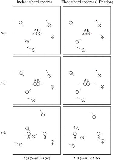
Figure 1: Sketch of the microscopic dynamics of inelastic hard spheres (IHS, left panel) and elastic hard spheres under a friction force (EHS, right panel). At $t=0^{-}$ both systems are prepared in the same microstate and particles A and B are about to collide. In the IHS system, particles A and B recede immediately after collision (at $t=0^{+}$) with a relative velocity smaller than the pre-collision one, so the mean kinetic energy decreases, $E(0^{+})<E(0^{-})$. During the time step $\delta t$ no collision takes place and the particles move ballistically, so $E(\delta t)=E(0^{+})$. In the EHS system, the collision between particles A and B is elastic, so $E(0^{+})=E(0^{-})$. However, during the time step $\delta t$ all the particles feel the drag force and, consequently, $E(\delta t)<E(0^{+})$. Note that at $t=\delta t$ the respective microstates in the IHS and EHS systems are different, even if the energy loss $E(0^{-})-E(\delta t)$ is the same.

Despite the trivial common structure of the macroscopic balance equations (6)–(8) for the free IHS and the driven EHS gases, the underlying microscopic dynamics is physically quite different in both systems: in the IHS gas (i) each colliding pair loses energy upon collision but (ii) all the particles move freely between two successive collisions; in the EHS case, however, (i) energy is conserved by collisions but (ii) all the particles lose energy between collisions due to the action of the drag force. Therefore, during a certain small time step, only a small fraction of particles is responsible for the cooling of the system in the IHS case, whereas all the particles contribute to the cooling in the EHS case. These differences are sketched in Fig. 1. In principle, there is no reason to expect that the relevant nonequilibrium physical properties (e.g., the one-particle velocity distribution function) are similar for IHS and frictional EHS under the same conditions.

Let us consider, for instance, the homogeneous cooling state vNE98 . In that case, the energy balance equation (8) becomes

$$\frac{\text{d}T_{\text{hc}}(t)}{\text{d}t}=-\zeta_{\text{hc}}(t)T_{\text{hc}}(t).$$ (9)

The solution to Eq. (9) is Haff’s law:

$$T_{\text{hc}}(t)=\frac{T_{\text{hc}}(0)}{\left[1+\frac{1}{2}\zeta_{\text{hc}}(0)t\right]^{2}},$$ (10)

where we have taken into account that $\zeta_{\text{hc}}(t)\propto T_{\text{hc}}^{1/2}(t)$. The above cooling law is valid for the homogeneous cooling state of both IHS and frictional EHS, provided that in the latter one considers a time-dependent friction coefficient $\gamma\propto T^{1/2}$ and $\gamma(0)=\zeta_{\text{hc}}(0)$. The homogeneous Boltzmann equation admits in both cases a scaling solution of the form

$$\begin{array}[]{c}f_{\text{hc}}(\mathbf{v},t)=n\left[{m}/{2T_{\text{hc}}(t)}\right]^{d/2}f_{\text{hc}}^{*}\left(\mathbf{c}(t)\right),\\ \mathbf{c}(t)=\mathbf{v}/\sqrt{2T_{\text{hc}}(t)/m}.\end{array}$$ (11)

On the other hand, while the distribution function is a Gaussian $f_{\text{hc}}^{*}(\mathbf{c})=\pi^{-d/2}\text{$e$}^{-c^{2}}$ for EHS GSB90 , deviations from a Gaussian are present in the case of IHS vNE98 ; BRC96 ; MS00 . These deviations are measured, for instance, by a nonzero fourth cumulant (or kurtosis),

$$a_{2}\equiv\frac{4}{d(d+2)}\langle c^{4}\rangle-1,$$ (12)

and by an overpopulated high-energy tail $f_{\text{hc}}^{*}(\mathbf{c})\sim\text{$e$}^{-Ac}$. In the case of a gas heated by a white-noise forcing, the steady-state distribution function is again a Gaussian for frictional EHS, while $a_{2}\neq 0$ and $f^{*}(\mathbf{c})\sim\text{$e$}^{-Ac^{3/2}}$ for IHS vNE98 ; MS00 .

The above two examples are sufficient to illustrate that, obviously, the IHS and driven EHS systems are not strictly equivalent. On the other hand, the differences between the homogeneous solutions for IHS and EHS are not quantitatively important in the domain of thermal speeds (for instance, $|a_{2}|\lesssim 0.02$ for IHS with $\alpha\gtrsim 0.7$). Therefore, it is still possible that both systems exhibit comparable departures from equilibrium in inhomogeneous states, in which case transport of momentum and/or energy are the most relevant phenomena. As a matter of fact, one of the most distinctive features of granular gases, namely the clustering instability, has a hydrodynamic origin G03 ; BRC96 , and so it must also appear in a gas of EHS under the action of a drag force with a state-dependent friction coefficient $\gamma$ proportional to a characteristic local collision frequency.

The aim of this paper is to investigate to what extent a frictional EHS gas can “disguise” as an IHS gas in what concerns the transport properties of mass, momentum, and/or energy, which are dominated by the thermal domain of the velocity distribution function. If that were the case, the significant body of work already available for the kinetic theory of normal gases could be exploited to provide a practical tool for granular gases. A preliminary report of this work has been given in Ref. AS04 . In Sec. II we construct a minimal model of EHS in the framework of the Boltzmann equation that intends to capture the basic properties of the Boltzmann equation for IHS with a given coefficient of restitution $\alpha$. First, as discussed above, the EHS system is assumed to be under the influence of a drag force. By equating the right-hand sides of Eqs. (4) and (5), the friction coefficient $\gamma$ of the EHS gas should be chosen as half the cooling rate $\zeta(\alpha)$ of the true IHS gas. However, this is not practical since $\zeta$ is a functional of the nonequilibrium velocity distribution of IHS and we want an autonomous Boltzmann equation for EHS, i.e., an equation that does not require the previous knowledge of the solution of the Boltzmann equation for IHS. One could autonomously define $\gamma$ as the same functional of the EHS distribution as $\zeta$ is of the IHS distribution, but this would also result in a too complicated model. For these reasons, we choose $\gamma=\frac{1}{2}\zeta_{0}(\alpha)$, where $\zeta_{0}$ is the cooling rate in the local equilibrium approximation. This is consistent with the fact that the velocity distribution function of EHS is a Gaussian in the homogeneous cooling state, as well as in the steady state driven by a white-noise thermostat. The price to be paid by the simple choice $\gamma=\frac{1}{2}\zeta_{0}$ is that the equivalence between the respective sources of cooling, Eqs. (4) and (5), is only approximate. As a second ingredient of the model, the collision rate of the EHS gas, relative to that of the IHS gas, defines a dimensionless parameter $\beta$ that can be freely chosen to optimize the agreement with the IHS properties. In order to have a clue on an optimal choice of $\beta$, the Navier–Stokes transport coefficients of both systems are compared in Sec. III. As a compromise between simplicity and accuracy, we simply choose $\beta(\alpha)=\frac{1}{2}(1+\alpha)$. The (approximate) mapping EHS$\rightarrow$IHS allows one to extend directly to granular gases those kinetic models originally proposed for conventional gases C88 ; GS03 . This is illustrated in Sec. IV for the Bhatnagar–Gross–Krook BGK54 and the ellipsoidal statistical H66 kinetic models. The extension of the approximate equivalence between inelastic and (frictional) elastic particles to mixtures, dense gases, and Maxwell models is discussed in Appendices A–C, respectively. In particular, the applications to mixtures and to dense gases reinforce the choice $\beta(\alpha)=\frac{1}{2}(1+\alpha)$. The paper ends with some concluding remarks in Sec. V.

II Model of frictional elastic hard spheres

II.1 Basic properties of the Boltzmann equation for inelastic hard spheres

The Boltzmann equation for a gas of inelastic hard spheres (IHS) is GS95 ; BDS97 ; vNE01

$$\left(\partial_{t}+{\bf v\cdot\nabla}\right)f=J^{(\alpha)}[f,f],$$ (13)

where $f({\bf r},{\bf v};t)$ is the one-particle velocity distribution function and $J^{(\alpha)}[f,f]$ is the Boltzmann collision operator

$$J^{(\alpha)}[f,f]=\sigma^{d-1}\int\text{d}{\bf v}_{1}\int\text{d}\widehat{\bm{\sigma}}\,\Theta({\bf g}\cdot\widehat{\bm{\sigma}})({\bf g}\cdot\widehat{\bm{\sigma}})$$

$$\times\left[\alpha^{-2}f({\bf v}^{\prime\prime})f({\bf v}_{1}^{\prime\prime})-f({\bf v})f({\bf v}_{1})\right],$$ (14)

where the explicit dependence of $f$ on ${\bf r}$ and $t$ has been omitted. In Eq. (14), $\sigma$ is the diameter of a sphere and $\Theta$ is the Heaviside step function. The pre-collisional or restituting velocities ${\bf v}^{\prime\prime}$ and ${\bf v}_{1}^{\prime\prime}$ are given by Eq. (3). Of course, the collision operator for elastic hard spheres (EHS), $J^{(1)}[f,f]$, is obtained from Eqs. (14) and (3) by simply setting $\alpha=1$.

The first $d+2$ moments of the velocity distribution function define the number density

$$n(\mathbf{r},t)=\int\text{d}\mathbf{v}\,f({\bf r},{\bf v};t),$$ (15)

the nonequilibrium flow velocity

$$\mathbf{u}(\mathbf{r},t)=\frac{1}{n(\mathbf{r},t)}\int\text{d}\mathbf{v}\,\mathbf{v}f({\bf r},{\bf v};t)=\langle\mathbf{v}\rangle,$$ (16)

and the granular temperature

$$T(\mathbf{r},t)=\frac{m}{n(\mathbf{r},t)d}\int\text{d}\mathbf{v}\,V^{2}(\mathbf{r},t)f({\bf r},{\bf v};t)=\frac{m\langle V^{2}\rangle}{d},$$ (17)

where ${\bf V}({\bf r},t)\equiv{\bf v}-{\bf u}({\bf r},t)$ is the peculiar velocity. The basic properties of $J^{(\alpha)}[f,f]$ are those that determine the form of the macroscopic balance equations for mass, momentum, and energy,

$$\int\text{d}{\bf v}\left(\begin{array}[]{c}1\\ m{\bf v}\\ \frac{1}{2}mV^{2}\end{array}\right)J^{(\alpha)}[f,f]=\left(\begin{array}[]{c}0\\ {\bf 0}\\ -\frac{d}{2}nT\zeta\end{array}\right).$$ (18)

By standard manipulations of the collision operator, the cooling rate can be written as BDS97 ; BDS99

$$\zeta(\mathbf{r},t)=(1-\alpha^{2})\frac{m\pi^{\frac{d-1}{2}}\sigma^{d-1}}{4d\Gamma\left(\frac{d+3}{2}\right)}\frac{n(\mathbf{r},t)}{T(\mathbf{r},t)}\langle V_{12}^{3}\rangle,$$ (19)

where

$$\langle V_{12}^{3}\rangle=\frac{1}{n^{2}(\mathbf{r},t)}\int\text{d}{\bf v}_{1}\int\text{d}{\bf v}_{2}\,|{\bf v}_{1}-{\bf v}_{2}|^{3}f({\bf r},{\bf v}_{1};t)f({\bf r},{\bf v}_{2};t)$$ (20)

is the average value of the cube of the relative speed. The properties (18) lead to the balance equations (6)–(8) with the following kinetic expressions for the pressure tensor and the heat flux,

$$P_{ij}=m\int\text{d}\mathbf{v}\,V_{i}V_{j}f(\mathbf{v}),$$ (21)

$$\mathbf{q}=\frac{m}{2}\int\text{d}\mathbf{v}\,V^{2}\mathbf{V}f(\mathbf{v}).$$ (22)

The cooling rate $\zeta$ is a nonlinear functional of the distribution function $f$ through the average $\langle V_{12}^{3}\rangle$. As a consequence, $\zeta$ cannot be explicitly evaluated unless the Boltzmann equation is solved. Nevertheless, a simple estimate is obtained from Eq. (20) by replacing the actual distribution function $f$ by the local equilibrium distribution

$$f_{0}(\mathbf{v})=n(m/2\pi T)^{d/2}\exp(-mV^{2}/2T).$$ (23)

In that case,

$$\langle V_{12}^{3}\rangle \to \langle V_{12}^{3}\rangle_{0}=2^{3/2}\langle V^{3}\rangle_{0}$$ (24)

$$= 4\pi^{-d/2}\Omega_{d}\Gamma\left(\frac{d+3}{2}\right)\left(\frac{T}{m}\right)^{3/2},$$

where $\Omega_{d}\equiv 2\pi^{d/2}/\Gamma(d/2)$ is the total solid angle. When the approximation (24) is inserted into Eq. (19), one gets the local equilibrium cooling rate BDS99 ; BDKS98

$$\zeta_{0}(\mathbf{r},t)=\zeta_{0}^{*}\nu_{0}(\mathbf{r},t),\quad\zeta_{0}^{*}\equiv\frac{d+2}{4d}(1-\alpha^{2}),$$ (25)

where

$$\nu_{0}=\frac{4\Omega_{d}}{\sqrt{\pi}(d+2)}n\sigma^{d-1}\left(\frac{T}{m}\right)^{1/2}$$ (26)

is an effective collision frequency. The local equilibrium estimate (25) expresses the cooling rate as a functional of $f$ through the local density and temperature only. In addition, its dependence on inelasticity is simply $\zeta_{0}\propto 1-\alpha^{2}$.

It is now convenient to introduce the modified collision operator BDS99

$$\bar{J}^{(\alpha)}[f,f]\equiv J^{(\alpha)}[f,f]-\frac{\zeta}{2}\frac{\partial}{\partial{\bf v}}\cdot\left({\bf V}f\right).$$ (27)

By construction, the operator $\bar{J}^{(\alpha)}[f,f]$ has the properties

$$\int\text{d}{\bf v}\left(\begin{array}[]{c}1\\ m{\bf v}\\ \frac{1}{2}mV^{2}\end{array}\right)\bar{J}^{(\alpha)}[f,f]=\left(\begin{array}[]{c}0\\ {\bf 0}\\ 0\end{array}\right),$$ (28)

as follows from direct evaluation using Eq. (18).

II.2 The model

The modified inelastic collision operator $\bar{J}^{(\alpha)}[f,f]$ shares with the elastic collision operator $J^{(1)}[f,f]$ the property of having $d+2$ vanishing low velocity moments. Of course, $\bar{J}^{(\alpha)}[f,f]$ and $J^{(1)}[f,f]$ differ in many other aspects. For instance, in the homogeneous cooling state the velocity distribution function is the solution to $\bar{J}^{(\alpha)}[f_{\text{hc}},f_{\text{hc}}]=0$ BDS99 , which differs from a Gaussian, the latter being the solution to ${J}^{(1)}[f,f]=0$. Moreover, the elastic collision operator satisfies the H-theorem, namely

$$\int\text{d}\mathbf{v}(\ln f){J}^{(1)}[f,f]\leq 0,$$ (29)

while an H-theorem has not been proven for $\bar{J}^{(\alpha)}[f,f]$. Despite these differences, the common properties (28) suggest the possibility that the operators $\bar{J}^{(\alpha)}[f,f]$ and ${J}^{(1)}[f,f]$ have a similar behavior in the domain of thermal speeds (i.e., for $V\lesssim 2\sqrt{2T/m}$). This expectation can be exploited to propose the approximation

$$\bar{J}^{(\alpha)}[f,f]\to\beta J^{(1)}[f,f],$$ (30)

where $\beta(\alpha)$ is a positive constant to be determined later on. Its introduction does not invalidate Eq. (28) but allows us to fine-tune the approximate equivalence between both operators. In agreement with the spirit of the above discussion we further approximate the true cooling rate given by Eq. (19) by the local equilibrium estimate (25). In summary, our model consists of the replacement

$$J^{(\alpha)}[f,f]\to\beta J^{(1)}[f,f]+\frac{\zeta_{0}}{2}\frac{\partial}{\partial{\bf v}}\cdot\left({\bf V}f\right),$$ (31)

so that the Boltzmann equation (13) becomes

$$\left(\partial_{t}+{\bf v\cdot\nabla}-\frac{\zeta_{0}}{2}\frac{\partial}{\partial{\bf v}}\cdot{\bf V}\right)f=\beta J^{(1)}[f,f].$$ (32)

In this model, the gas of inelastic hard spheres with a given coefficient of restitution $\alpha$ is replaced by an “equivalent” gas of elastic hard spheres subject to the action of a drag force $\mathbf{F}_{\text{drag}}=-m\gamma\mathbf{V}$ with $\gamma=\frac{1}{2}\zeta_{0}$. While this drag force does not affect the conservation of momentum on average, this is not so at a microscopic level. To clarify this point, let us consider the particles inside a small box $\delta\mathbf{r}$ centered about the point $\mathbf{r}$ at time $t$ in a given microstate. Because of the action of the drag force, the velocities of those particles change during a short time interval $\delta t$ as

$$\mathbf{v}_{i}(t)\to\mathbf{v}_{i}(t+\delta t)=\mathbf{v}_{i}(t)-\gamma(\mathbf{r},t)\left[\mathbf{v}_{i}(t)-\mathbf{u}(\mathbf{r},t)\right]\delta t.$$ (33)

Summing over all the $\delta N$ particles inside the box, we find that, in general, $\sum_{i\in\delta\mathbf{r}}\mathbf{v}_{i}(t+\delta t)\neq\sum_{i\in\delta\mathbf{r}}\mathbf{v}_{i}(t)$ since $\sum_{i\in\delta\mathbf{r}}\mathbf{v}_{i}(t)\neq\delta N\mathbf{u}(\mathbf{r},t)$. On the other hand, the momentum is conserved when averaging over all the microstates, i.e., $\langle\sum_{i\in\delta\mathbf{r}}\mathbf{v}_{i}(t+\delta t)\rangle=\langle\sum_{i\in\delta\mathbf{r}}\mathbf{v}_{i}(t)\rangle$, where we have taken into acoount that, by definition, $\mathbf{u}(\mathbf{r},t)=\langle\sum_{i\in\delta\mathbf{r}}\mathbf{v}_{i}(t)\rangle/\langle\delta N\rangle$. This averaging process is already built in the Boltzmann equation (32).

The fact that in the friction constant the actual cooling rate $\zeta$ of the granular gas is approximated by $\zeta_{0}$ (or, equivalently, $\langle V_{12}^{3}\rangle\to\langle V_{12}^{3}\rangle_{0}$) is dictated by simplicity since it does not seem necessary to retain the detailed functional dependence of Eq. (20) when on the other hand the coarse-grained approximation (30) is being used. In other words, the discrepancies due to $\zeta\to\zeta_{0}$ may be expected to be less important than those associated with the approximation (30) itself. In any case, if one wishes to keep the true cooling rate $\zeta$ in the model (31), $\zeta$ must be interpreted as a functional of the solution of Eq. (32) itself, not as a functional of the solution of Eq. (13). Otherwise, Eq. (32) would not be an autonomous equation and it would be necessary to know the solution of the IHS Boltzmann equation (13) before dealing with the EHS Boltzmann equation (32), what is not only impractical but artificially complicated as well.

In Eq. (14) the coefficient of restitution $\alpha$ appears both explicitly (by the factor $\alpha^{-2}$ inside the collision integral) and implicitly [through the collision rule (3)]. In contrast, in the model (31) $\alpha$ appears only explicitly, as well as outside the collision integral, through the approximate cooling rate $\zeta_{0}\propto 1-\alpha^{2}$ and the parameter $\beta(\alpha)$ still to be determined. This simplification can be justified as long as one is mainly interested in the gross effects of inelasticity on the nonequilibrium velocity distribution function, while the fine details might not be captured by the model (31). However, as seen in the companion paper AS05 , the reliability of the EHS model turns out to be higher than the expected one.

In principle, there is no reason to expect that the gas of EHS which most efficiently mimics the relevant transport properties of the granular gas is made of particles with a diameter $\sigma^{\prime}$ equal to the diameter $\sigma$ of the inelastic spheres. If $\sigma^{\prime}$ and $\sigma$ were equal, then both systems would have the same mean free time but not necessarily the same rate of momentum and energy transfer upon collisions. The effect associated with $\sigma^{\prime}\neq\sigma$ is accounted for by the parameter $\beta$. Since $J^{(1)}[f,f]$ is defined by setting $\alpha=1$ in Eq. (14), it is proportional to $\sigma^{d-1}$, not to ${\sigma^{\prime}}^{d-1}$. Therefore, $\beta J^{(1)}[f,f]$ is the collision operator of EHS of diameter $\sigma^{\prime}=\beta^{1/(d-1)}\sigma$. Alternatively, Eq. (32) can be rewritten as

$$\left(\partial_{t^{\prime}}+{\bf v\cdot\nabla^{\prime}}-\frac{\zeta_{0}}{2\beta}\frac{\partial}{\partial{\bf v}}\cdot{\bf V}\right)f=J^{(1)}[f,f],$$ (34)

where $t^{\prime}\equiv\beta t$ and $\nabla^{\prime}=\partial/\partial{\mathbf{r}^{\prime}}$ with $\mathbf{r}^{\prime}\equiv\beta\mathbf{r}$. According to Eq. (34), the original IHS system is replaced by an EHS system with the same diameter $\sigma^{\prime}=\sigma$, but with a friction constant $\gamma^{\prime}=\zeta_{0}/2\beta$ and spatial and temporal variables scaled by a factor $\beta$ with respect to those of the IHS system. In what follows, we will use for the model the form (32) rather than the form (34) and will view $\beta$ as a correction factor to modify the collision rate of the equivalent system of EHS, relative to the collision rate of the IHS system. This implies that after a certain common time interval $\Delta t$ the number of collisions experienced by the EHS is in general different from that of the IHS. In the next Section we make a definite proposal for $\beta(\alpha)$ based on the comparison between the EHS and IHS Navier–Stokes transport coefficients.

III Navier–Stokes transport coefficients

III.1 Stress tensor and heat flux

The irreversible momentum and energy transport are measured by the stress tensor $\Pi_{ij}=P_{ij}-p\delta_{ij}$ (where $p=nT={d}^{-1}\text{Tr}\,\mathsf{P}$ is the hydrostatic pressure) and the heat flux $\mathbf{q}$. By an extension of the Chapman–Enskog method CC70 to the case of inelastic collisions BDKS98 ; GD99 ; BC01 ; GM02 ; S03 , one gets the Navier–Stokes constitutive equations

$$\Pi_{ij}=-\eta\left(\nabla_{i}u_{j}+\nabla_{j}u_{i}-\frac{2}{d}\nabla\cdot\mathbf{u}\,\delta_{ij}\right),$$ (35)

$$\mathbf{q}=-\lambda\nabla T-\mu\nabla n,$$ (36)

where $\eta$ is the shear viscosity, $\lambda$ is the thermal conductivity, and $\mu$ is a transport coefficient with no counterpart in the elastic case. For IHS, the explicit expressions for the transport coefficients in the first Sonine approximation are given by BDKS98 ; BC01

$$\eta=\frac{nT}{\nu_{0}}\frac{1}{\nu_{\eta}^{*}-\frac{1}{2}\zeta^{*}},$$ (37)

$$\lambda=\frac{nT}{m\nu_{0}}\frac{d+2}{2}\frac{1+2a_{2}^{\text{hc}}}{\nu_{\lambda}^{*}-2\zeta^{*}},$$ (38)

$$\mu=\frac{T^{2}}{m\nu_{0}}\frac{d+2}{2}\frac{\zeta^{*}+a_{2}^{\text{hc}}\nu_{\lambda}^{*}}{(\nu_{\lambda}^{*}-\frac{3}{2}\zeta^{*})(\nu_{\lambda}^{*}-2\zeta^{*})}.$$ (39)

In these equations, the effective collision frequency $\nu_{0}$ is defined by Eq. (26),

$$a_{2}^{\text{hc}}=\frac{16(1-\alpha)(1-2\alpha^{2})}{9+24d-\alpha(41-8d)+30\alpha^{2}(1-\alpha)}$$ (40)

is an estimate of the kurtosis of the velocity distribution function [cf. Eq. (12)] in the homogeneous cooling state vNE98 ; note , and

$$\zeta^{*}=\zeta_{0}^{*}\left(1+\frac{3}{16}a_{2}^{\text{hc}}\right)$$ (41)

is the (reduced) cooling rate in the same state. Moreover,

$$\nu_{\eta}^{*} = \frac{\int\text{d}\mathbf{v}\,\mathsf{D}:{\cal L}^{(\alpha)}f_{0}\mathsf{D}}{\nu_{0}\int\text{d}\mathbf{v}\,f_{0}\mathsf{D}:\mathsf{D}}$$ (42)

$$= \frac{3}{4d}\left(1-\alpha+\frac{2}{3}d\right)(1+\alpha)\left(1-\frac{1}{32}a_{2}^{\text{hc}}\right)$$

is the (reduced) collision frequency associated with the shear viscosity, where

$${D}_{ij}(\mathbf{V})\equiv m\left(V_{i}V_{j}-\frac{V^{2}}{d}\delta_{ij}\right),$$ (43)

and

$$\nu_{\lambda}^{*} = \frac{\int\text{d}\mathbf{v}\,\mathbf{S}\cdot{\cal L}^{(\alpha)}f_{0}\mathbf{S}}{\nu_{0}\int\text{d}\mathbf{v}\,f_{0}\mathbf{S}\cdot\mathbf{S}}$$ (44)

$$= \frac{1+\alpha}{d}\left[\frac{d-1}{2}+\frac{3}{16}(d+8)(1-\alpha)\right.$$

$$\left.+\frac{4+5d-3(4-d)\alpha}{512}a_{2}^{\text{hc}}\right]$$

is the (reduced) collision frequency associated with the thermal conductivity, where

$$\mathbf{S}(\mathbf{V})\equiv\left(\frac{m}{2}V^{2}-\frac{d+2}{2}T\right)\mathbf{V}.$$ (45)

In the first equalities of Eqs. (42) and (44), ${\cal L}^{(\alpha)}$ represents the linearization of the collision operator $J^{(\alpha)}$ around the homogeneous cooling state:

$${\cal L}^{(\alpha)}\phi\equiv-J^{(\alpha)}[\phi,f_{\text{hc}}]-J^{(\alpha)}[f_{\text{hc}},\phi].$$ (46)

In the model (31) the transport coefficients are formally given by Eqs. (37)–(39), except that $a_{2}^{\text{hc}}\to 0$ (since the homogeneous cooling state solution is now the local equilibrium distribution, i.e., $f_{\text{hc}}=f_{0}$) and $\nu_{\eta}^{*}$ and $\nu_{\lambda}^{*}$ are given by the first equalities of Eqs. (42) and (44) with the replacement

$${\cal L}^{(\alpha)}\to\beta{\cal L}^{(1)}-\frac{\zeta_{0}}{2}\frac{\partial}{\partial\mathbf{v}}\cdot\mathbf{V},$$ (47)

where the operator $\mathcal{L}^{(1)}$ is defined by Eq. (46) with $\alpha=1$ and $f_{\text{hc}}=f_{0}$. Taking into account the properties

$$\mathbf{V}\cdot\partial_{\mathbf{v}}D_{ij}=2D_{ij},\quad\mathbf{V}\cdot\partial_{\mathbf{v}}S_{i}=3S_{i}+(d+2)TV_{i},$$ (48)

one easily gets

$$\nu_{\eta}^{*}\to\beta+\zeta_{0}^{*},$$ (49)

$$\nu_{\lambda}^{*}\to\frac{d-1}{d}\beta+\frac{3}{2}\zeta_{0}^{*}.$$ (50)

In summary, the transport coefficients of the EHS model in the first Sonine approximation are

$$\eta=\frac{nT}{\nu_{0}}\frac{1}{\beta+\frac{1}{2}\zeta_{0}^{*}},$$ (51)

$$\lambda=\frac{nT}{m\nu_{0}}\frac{d+2}{2}\frac{1}{\frac{d-1}{d}\beta-\frac{1}{2}\zeta_{0}^{*}},$$ (52)

$$\mu=\frac{T^{2}}{m\nu_{0}}\frac{d(d+2)}{2(d-1)}\frac{\zeta_{0}^{*}}{\beta(\frac{d-1}{d}\beta-\frac{1}{2}\zeta_{0}^{*})}.$$ (53)

So far, the choice of the parameter $\beta$ remains open. To reproduce the main trends in the $\alpha$-dependence of the shear viscosity for IHS, let us equate Eq. (51) to Eq. (37) (with $a_{2}^{\text{hc}}=0$ for consistency). This yields

$$\beta=\frac{1+\alpha}{2}\left[1-\frac{d-1}{2d}(1-\alpha)\right]\equiv\beta_{\eta}.$$ (54)

Analogously, the model captures the behavior of the thermal conductivity if $\beta$ is obtained by equating Eq. (52) to Eq. (38) with $a_{2}^{\text{hc}}=0$. The result is

$$\beta=\frac{1+\alpha}{2}\left[1+\frac{3}{8}\frac{4-d}{d-1}(1-\alpha)\right]\equiv\beta_{\lambda}.$$ (55)

This expression also optimizes the agreement between Eqs. (39) and (53), i.e., $\beta_{\mu}=\beta_{\lambda}$.

III.2 Self-diffusion

If in the homogeneous cooling state a group of tagged particles (here labeled with the subscript t) have initially a nonuniform density $n_{\text{t}}$, the associated velocity distribution function $f_{\text{t}}$ obeys the Boltzmann–Lorentz equation

$$\left(\partial_{t}+\mathbf{v}\cdot\nabla\right)f_{\text{t}}=J^{(\alpha)}[f_{\text{t}},f_{\text{hc}}]\equiv-\mathcal{L}^{(\alpha)}_{\text{BL}}f_{\text{t}}.$$ (56)

As a consequence, a current $\mathbf{j}_{\text{t}}=\int\text{d}\mathbf{v}\,\mathbf{v}f_{\text{t}}(\mathbf{v})$ of tagged particles appears opposing the concentration gradient. Conservation of the number of tagged particles implies the continuity equation

$$\partial_{t}n_{\text{t}}+\nabla\cdot\mathbf{j}_{\text{t}}=0.$$ (57)

In the limit of weak gradients, one has

$$\mathbf{j}_{\text{t}}=-D\nabla n_{\text{t}},$$ (58)

where $D$ is the self-diffusion coefficient. By standard application of the Chapman–Enskog method in the first Sonine approximation, the self-diffusion coefficient of IHS can be derived. The result is BRCG00

$$D=\frac{T}{m\nu_{0}}\frac{1}{\nu_{D}^{*}-\frac{1}{2}\zeta^{*}},$$ (59)

where

$$\nu_{D}^{*} = \frac{\int\text{d}\mathbf{v}\,\mathbf{v}\cdot{\cal L}_{\text{BL}}^{(\alpha)}f_{0}\mathbf{v}}{\nu_{0}\int\text{d}\mathbf{v}\,v^{2}f_{0}}$$ (60)

$$= \frac{d+2}{4d}(1+\alpha)\left(1-\frac{1}{32}a_{2}^{\text{hc}}\right)$$

is the (reduced) collision frequency associated with the self-diffusion coefficient.

In our EHS model, the Boltzmann–Lorentz equation (56) is replaced by

$$\left[\partial_{t}+\mathbf{v}\cdot\nabla-\frac{\zeta_{0}}{2}\frac{\partial}{\partial\mathbf{v}}\cdot\left(\mathbf{v}-\mathbf{u}_{\text{t}}\right)\right]f_{\text{t}} = \beta J^{(1)}[f_{\text{t}},f_{0}]$$ (61)

$$\equiv -\beta\mathcal{L}^{(1)}_{\text{BL}}f_{\text{t}},$$

where we have taken into account that the peculiar velocity $\mathbf{V}$ appearing on the left-hand side of Eq. (31) must now be understood as $\mathbf{v}-\mathbf{u}_{\text{t}}$, where $\mathbf{u}_{\text{t}}=\mathbf{j}_{\text{t}}/n_{\text{t}}$ is the mean velocity of the tagged particles, in order to make Eq. (61) consistent with the continuity equation (57). Similarly to Eq. (47), the model implies

$${\cal L}_{\text{BL}}^{(\alpha)}\to\beta{\cal L}_{\text{BL}}^{(1)}-\frac{\zeta_{0}}{2}\frac{\partial}{\partial\mathbf{v}}\cdot\mathbf{v},$$ (62)

so that

$$\nu^{*}_{D}\to\beta\frac{d+2}{2d}+\frac{\zeta_{0}^{*}}{2}.$$ (63)

In addition, the presence of the term proportional to $\mathbf{u}_{t}$ in Eq. (61) generates an extra term in the Chapman–Enskog method such that $\zeta^{*}/2$ in the denominator of Eq. (59) is replaced by $\zeta_{0}^{*}$. In summary, the self-diffusion coefficient corresponding to the EHS model is (in the first Sonine approximation)

$$D=\frac{T}{m\nu_{0}}\frac{1}{\frac{d+2}{2d}\beta-\frac{1}{2}\zeta_{0}^{*}}.$$ (64)

Identifying Eq. (64) with Eq. (59) (by setting $a_{2}^{\text{hc}}=0$ in the latter), one gets

$$\beta=\frac{1+\alpha}{2}\equiv\beta_{D}.$$ (65)

III.3 Comparison between the IHS and EHS transport coefficients

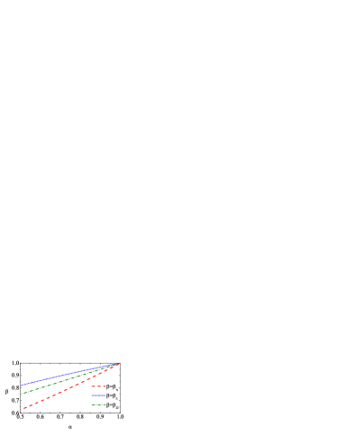
Figure 2: (Color online) Plot of $\beta_{\eta}$ (– – –), $\beta_{\lambda}$ ($\cdots$), and $\beta_{D}$ (– $\cdot$ – $\cdot$ –) as functions of the coefficient of restitution $\alpha$ in the three-dimensional case.

We have just seen that the suitable choice for the parameter $\beta(\alpha)$ under the criterion of optimizing the agreement with the transport coefficients of IHS is not unique. Depending on the transport property of interest, it may be more convenient $\beta=\beta_{\eta}$, $\beta=\beta_{\lambda}$, $\beta=\beta_{D}$, or even a different choice. Focusing on these three possibilities, we note that $\beta_{\eta}<\beta_{D}<\beta_{\lambda}$ for $d=2$ and $d=3$. Moreover, $\beta_{\lambda}<1$ for all $\alpha$ in the case $d=3$, as shown in Fig. 2. This indicates that the diameter of the equivalent EHS system is smaller than that of the actual IHS system ($\sigma^{\prime}<\sigma$), this effect being more pronounced with $\beta=\beta_{\eta}$ than with $\beta=\beta_{\lambda}$.

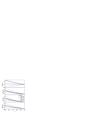
Figure 3: (Color online) Plot of the (reduced) shear viscosity $\eta/(nT/\nu_{0})$, thermal conductivity $\lambda/(nT/m\nu_{0})$, transport coefficient $\mu/(T^{2}/m\nu_{0})$, and self-diffusion coefficient $D/(T/m\nu_{0})$ for three-dimensional IHS (—) and the “equivalent” system of EHS with $\beta=\beta_{\eta}$ (– – –), $\beta=\beta_{\lambda}$ ($\cdots$), $\beta=\beta_{D}$ (– $\cdot$ – $\cdot$ –), and $\beta=1$ (– $\cdot\cdot$ – $\cdot\cdot$ –) as functions of the coefficient of restitution $\alpha$. Note that in the top panel the IHS curve and the EHS curve with $\beta=\beta_{\eta}$ are practically indistinguishable. The same happens in the bottom panel between the IHS curve and the EHS curve with $\beta=\beta_{D}$.

Figure 3 compares the four transport coefficients of IHS ($d=3$) [Eqs. (37)–(39) and (59)] with those of the “equivalent” system of EHS [Eqs. (51)–(53) and (64)] with the choices $\beta=\beta_{\eta}$ [Eq. (54)], $\beta=\beta_{\lambda}$ [Eq. (55)], $\beta=\beta_{D}$ [Eq. (65)], and $\beta=1$. It can be observed that the EHS shear viscosity combined with the choice $\beta=\beta_{\eta}$ reproduces almost perfectly the IHS shear viscosity. A similar situation occurs in the case of the self-diffusion coefficient with the choice $\beta=\beta_{D}$. This is because the influence of $a_{2}^{\text{hc}}\neq 0$ in the cooling rate $\zeta^{*}$ [Eq. (41)] and in the collision frequencies $\nu_{\eta}^{*}$ [Eq. (42)] and $\nu_{D}^{*}$ [Eq. (60)] is very small. On the other hand, the deviations of the EHS coefficients $\lambda$ and $\mu$ with $\beta=\beta_{\lambda}$ from the respective IHS coefficients are much more important, essentially due to the explicit dependence on $a_{2}^{\text{hc}}$ of the numerators on the right-hand sides of Eqs. (38) and (39), since the influence of $a_{2}^{\text{hc}}$ on $\nu_{\lambda}^{*}$ is again rather weak.

A natural question that arises is whether there exists a common choice for $\beta(\alpha)$ that reproduces reasonably well the $\alpha$-dependence of the four transport coefficients. Figure 3 shows that $\beta=\beta_{\eta}$, which is excellent in the case of $\eta$, strongly overestimates $\lambda$, $\mu$, and $D$. Moreover, $\beta=\beta_{\lambda}$ is not clearly superior to $\beta_{D}$ in the cases of $\lambda$ and $\mu$, whereas it is poorer in reproducing $\eta$ and $D$. Obviously, the naive choice $\beta=1$ does not capture well the $\alpha$-dependence of the transport coefficients, especially in the case of the shear viscosity. Therefore, we propose to take $\beta=\beta_{D}=\frac{1}{2}(1+\alpha)$. With this choice, the frictional gas of EHS has practically the same self-diffusion coefficient as the true IHS gas and similar values for the coefficients defining the heat flux. Although the choice $\beta=\frac{1}{2}(1+\alpha)$ underestimates the shear viscosity, this is not a serious drawback since this is the transport coefficient least sensitive to inelasticity. For instance, the ratio between the value of a transport coefficient at $\alpha=0.5$ and the value at $\alpha=1$ is about 1.3 in the case of $\eta$, while it is about 1.9 and 1.8 in the cases of $\lambda$ and $D$, respectively. At that rather high inelasticity ($\alpha=0.5$), the EHS transport coefficients with $\beta=\frac{1}{2}(1+\alpha)$ differ from the IHS ones by 14% ($\eta$), 2% ($\lambda$), 3% ($\mu$), and 0.5% ($D$).

There are two additional reasons to favor Eq. (65). First, it is much simpler than Eqs. (54) and (55) and does not depend on the dimensionality $d$. The second reason is more compelling. The extension of the model (31) to dilute mixtures and to dense gases is carried out in Appendices A and B, respectively. In both cases the equation for the collisional transfer of energy imposes the choice (65) as the most natural one, without having to resort to the evaluation of transport coefficients.

It is worth mentioning that the transport coefficients obtained from frictional EHS with $\gamma=\frac{1}{2}\zeta_{0}$ and $\beta=\frac{1}{2}(1+\alpha)$ exhibit a much better agreement with the IHS coefficients than the ones corresponding to the inelastic Maxwell model S03 . The relationship between the inelastic Maxwell model and the (frictional) elastic Maxwell model is discussed in Appendix C.

Before closing this Section, a comment is in order. The transport coefficients $\eta$, $\lambda$, $\mu$, and $D$ have been considered here in the first Sonine approximation, both for IHS and EHS, what has allowed us to work with explicit expressions. Without prejudicing the degree of reliability of the first Sonine approximation, it can be understood as a useful tool to probe the structure of the linearized collision operator through some relevant inner products [see the first equalities of Eqs. (42), (44), and (60)]. On the other hand, a comparison of the first Sonine approximation for the transport coefficients with direct simulation data shows a good agreement for $\eta$ BR04 ; MSG04 and $D$ BRCG00 ; GM04 , but important discrepancies for high inelasticity are present in the cases of $\lambda$ and $\mu$ BR04 ; MSG05 .

IV Kinetic modeling

IV.1 BGK model

The (approximate) mapping IHS$\leftrightarrow$EHS allows one to take advantage of the existence of simple models for EHS to extend them straightforwardly to IHS. For instance, consider the well-known Bhatnagar–Gross–Krook (BGK) model for elastic hard spheres BGK54 :

$$J^{(1)}[f,f]\to-\nu_{0}(f-f_{0}),$$ (66)

where $f_{0}$ is the local equilibrium distribution (23) and the effective collision frequency $\nu_{0}$ is usually identified with Eq. (26) in order to make the shear viscosity agree with that of the Boltzmann equation. Thus, in consistency with the approximation (31), the extension of the BGK model to inelastic hard spheres would simply be

$$J^{(\alpha)}[f,f]\to-\beta\nu_{0}(f-f_{0})+\frac{\zeta_{0}}{2}\frac{\partial}{\partial{\bf v}}\cdot\left({\bf V}f\right)$$ (67)

with $\zeta_{0}$ and $\beta$ given by Eqs. (25) and (65), respectively. In fact, the kinetic model (67) can be seen as a simplification of the one already proposed in Ref. BDS99 :

$$J^{(\alpha)}[f,f]\to-\beta\nu_{0}(f-f_{\text{hc}})+\frac{\zeta}{2}\frac{\partial}{\partial{\bf v}}\cdot\left({\bf V}f\right),$$ (68)

where here $f_{\text{hc}}$ represents the local form of the homogeneous cooling state, $\zeta$ is given by Eq. (41), and $\beta$ is assumed to be given by Eq. (54).

The linearized collision operator corresponding to the BGK model (67) is simply

$${\cal L}^{(\alpha)}\to\beta\nu_{0}-\frac{\zeta_{0}}{2}\frac{\partial}{\partial{\bf v}}\cdot{\bf V}.$$ (69)

As a consequence, the relation (49) holds again but one has $\nu_{\lambda}^{*}\to\beta+\frac{3}{2}\zeta_{0}^{*}$ instead of (50). Therefore, the shear viscosity is given by Eq. (51), while the thermal conductivity and the coefficient $\mu$ are

$$\lambda=\frac{nT}{m\nu_{0}}\frac{d+2}{2}\frac{1}{\beta-\frac{1}{2}\zeta_{0}^{*}},$$ (70)

$$\mu=\frac{T^{2}}{m\nu_{0}}\frac{d+2}{2}\frac{\zeta_{0}^{*}}{\beta(\beta-\frac{1}{2}\zeta_{0}^{*})},$$ (71)

which differ from Eqs. (52) and (53), respectively, by a factor $(d-1)/d$ in front of $\beta$.

In the case of self-diffusion in the homogeneous cooling state, the BGK kinetic equation for tagged particles is

$$\left[\partial_{t}+\mathbf{v}\cdot\nabla-\frac{\zeta_{0}}{2}\frac{\partial}{\partial\mathbf{v}}\cdot\left(\mathbf{v}-\mathbf{u}_{\text{t}}\right)\right]f_{\text{t}}=-\beta\nu_{0}\left(f_{\text{t}}-\frac{n_{\text{t}}}{n}f_{0}\right),$$ (72)

so the Boltzmann–Lorentz operator becomes

$${\cal L}_{\text{BL}}^{(\alpha)}\to\beta\nu_{0}-\frac{\zeta_{0}}{2}\frac{\partial}{\partial\mathbf{v}}\cdot\mathbf{v}$$ (73)

and one has $\nu_{D}^{*}\to\beta+\frac{3}{2}\zeta_{0}^{*}$ instead of (63). Thus,

$$D=\frac{T}{m\nu_{0}}\frac{1}{\beta-\frac{1}{2}\zeta_{0}^{*}},$$ (74)

which differs from Eq. (64).

The inability of the BGK model to reproduce simultaneously the different transport coefficients is already present in the elastic case and is the price to be paid by the inclusion of a single collision frequency $\nu_{0}$. In particular, the BGK model yields the value $\text{Pr}=1$ for the Prandtl number $\text{Pr}\equiv(d+2)\eta/2m\lambda$ in the elastic limit, while the correct Boltzmann value is (in the first Sonine approximation) $\text{Pr}=(d-1)/d$.

IV.2 Ellipsoidal statistical model

To avoid in part the above limitation, the so-called ellipsoidal statistical (ES) model was proposed about forty years ago for elastic particles C88 ; H66 . This kinetic model reads

$$J^{(1)}[f,f]\to-\nu_{0}\text{Pr}(f-f_{R}),$$ (75)

where

$$f_{R}(\mathbf{v})=n\left(\frac{mn}{2\pi}\right)^{d/2}\left(\det\mathsf{R}\right)^{-1/2}\exp\left(-\frac{mn}{2}\mathsf{R}^{-1}:\mathbf{V}\mathbf{V}\right)$$ (76)

is an anisotropic Gaussian distribution with the tensor $\mathsf{R}$ given by

$$\mathsf{R}=\frac{1}{\text{Pr}}\left[p\mathsf{I}-\left(1-\text{Pr}\right)\mathsf{P}\right],$$ (77)

$\mathsf{P}$ being the pressure tensor. The ES choice of $f_{R}$ is based on information theory arguments. Note that the ES model reduces to the conventional BGK model in the special case $\text{Pr}=1$. It is then convenient to consider Pr as a free parameter of the model so that the BGK model is recovered by formally setting $\text{Pr}=1$. The reference distribution $f_{R}$ has a finite norm provided that $\mathsf{R}$ is a positive definite matrix, i.e., its eigenvalues $r_{i}$ must be non-negative. From Eq. (77), $r_{i}=\text{Pr}^{-1}[p-(1-\text{Pr})p_{i}]$, where $p_{i}$ are the eigenvalues of the pressure tensor $\mathsf{P}$. Since $\sum_{i=1}^{d}p_{i}=dp$, then $p_{i}\leq dp$ and, consequently, the positiveness of $r_{i}$ implies that $\text{Pr}\geq({d-1})/d$. The lower bound coincides with the physical value of the Prandtl number. The first few moments of $f_{R}$ are

$$\int\text{d}\mathbf{v}\,\{1,\mathbf{V},m\mathbf{V}\mathbf{V}\}f_{R}(\mathbf{v})=\{n,\mathbf{0},\mathsf{R}\}.$$ (78)

While in the BGK equation (66) the reference function $f_{0}$ (namely, the local equilibrium distribution) is a functional of $f$ through its hydrodynamic fields $n$, $\mathbf{u}$, and $T$, in the ES model $f_{R}$ depends also on the irreversible part of the momentum flux.

When (75) is inserted into (31) we get our extension of the ES kinetic model for IHS:

$$J^{(\alpha)}[f,f]\to-\beta\nu_{0}\text{Pr}(f-f_{R})+\frac{\zeta_{0}}{2}\frac{\partial}{\partial{\bf v}}\cdot\left({\bf V}f\right).$$ (79)

We note that the ES model (79) is different from the more detailed Gaussian kinetic model recently proposed by Dufty et al. DBZ04 , the most important difference being that the collision frequency becomes a function of the peculiar velocity in the latter Gaussian model. The kinetic model (79) should also be distinguished from the ansatz of an anisotropic Gaussian (or maximum-entropy) velocity distribution function introduced by Jenkins and Richman JR88 as a means to obtain a closed set of equations for the pressure tensor.

The linearized collision operator associated with (79) is given by (47), where now the action of the linearized operator in the elastic case is GS03

$$\mathcal{L}^{(1)}\phi(\mathbf{v}) = \nu_{0}\left[\text{Pr}\phi(\mathbf{v})+\frac{1-\text{Pr}}{2pT}f_{0}(\mathbf{V})\mathsf{D}(\mathbf{V})\right.$$ (80)

$$\left.:\int\text{d}\mathbf{v}^{\prime}\,\mathsf{D}\left(\mathbf{V}^{\prime}\right)\phi(\mathbf{v}^{\prime})\right].$$

This implies that the shear viscosity is given by Eq. (51), while the thermal conductivity and the $\mu$ coefficient are

$$\lambda=\frac{nT}{m\nu_{0}}\frac{d+2}{2}\frac{1}{\text{Pr}\beta-\frac{1}{2}\zeta_{0}^{*}},$$ (81)

$$\mu=\frac{T^{2}}{m\nu_{0}}\frac{d+2}{2}\frac{\zeta_{0}^{*}}{\text{Pr}\beta(\text{Pr}\beta-\frac{1}{2}\zeta_{0}^{*})},$$ (82)

respectively. Equations (81) and (82) coincide with Eqs. (52) and (53) if one sets $\text{Pr}=(d-1)/d$. Of course, the BGK results (70) and (71) are recovered by formally setting $\text{Pr}=1$.

The natural version of the ES model to the self-diffusion problem is

$$\left[\partial_{t}+\mathbf{v}\cdot\nabla-\frac{\zeta_{0}}{2}\frac{\partial}{\partial\mathbf{v}}\cdot\left(\mathbf{v}-\mathbf{u}_{\text{t}}\right)\right]f_{\text{t}}=-\beta\nu_{0}\text{Pr}\left(f_{\text{t}}-\frac{n_{\text{t}}}{n}f_{0}\right).$$ (83)

Therefore,

$$D=\frac{T}{m\nu_{0}}\frac{1}{\text{Pr}\beta-\frac{1}{2}\zeta_{0}^{*}},$$ (84)

which differs from Eq. (64), unless one allows the Prandtl number to take the artificial value $\text{Pr}=(d+2)/2d$.

IV.3 Solution of the BGK and ES models for uniform shear flow

As an illustration of the BGK and ES models extended to IHS, let us analyze their solutions in the case of one of the paradigmatic nonequilibrium states, namely the uniform (or simple) shear flow. In most of this Subsection we will consider the nonlinear ES model (79) with an arbitrary value for Pr, so that $\text{Pr}=1$ corresponds to the BGK model and $\text{Pr}=(d-1)/d$ corresponds to the true ES model.

In the uniform shear flow, the density is constant, the granular temperature is uniform, and the flow velocity has a linear profile $\mathbf{u}=ay\widehat{\mathbf{x}}$, $a$ being the constant shear rate. At a more fundamental level, the velocity distribution function becomes uniform when the velocities are referred to the co-moving Lagrangian frame:

$$f(\mathbf{r},\mathbf{v};t)=f(\mathbf{V},t),\quad\mathbf{V}=\mathbf{v}-ay\widehat{\mathbf{x}}.$$ (85)

In that case, the ES model kinetic equation reads

$$\partial_{t}f-aV_{y}\frac{\partial}{\partial V_{x}}f-\frac{\zeta_{0}}{2}\frac{\partial}{\partial{\bf V}}\cdot\left({\bf V}f\right)=-\beta\nu_{0}\text{Pr}(f-f_{R}).$$ (86)

Multiplying both sides by $mV_{i}V_{j}$ and integrating over velocity, we get

$$\partial_{t}P_{ij}+a\left(\delta_{ix}P_{yj}+\delta_{jx}P_{iy}\right)+\zeta_{0}P_{ij}=-\beta\nu_{0}\left(P_{ij}-p\delta_{ij}\right),$$ (87)

where on the right-hand side we have made use of Eqs. (77) and (78). The set of equations (87) is common to the BGK and the ES models since the constant Pr does not appear. The structure of Eq. (87) is also obtained from other BGK-like models BMD96 ; BRM97 , as well as from the Boltzmann equation in Grad’s approximation G02 ; SGD03 . In this latter case, however, the flexibility of accommodating the coefficient $\beta$ disappears since by construction it is constrained to $\beta=\beta_{\eta}$.

The three independent equations stemming from Eq. (87) are

$$\partial_{t}p+\zeta_{0}p+\frac{2a}{d}P_{xy}=0,$$ (88)

$$\partial_{t}P_{xy}+\left(\beta\nu_{0}+\zeta_{0}\right)P_{xy}+aP_{yy}=0,$$ (89)

$$\partial_{t}P_{yy}+\left(\beta\nu_{0}+\zeta_{0}\right)P_{yy}-\beta\nu_{0}p=0.$$ (90)

Their steady-state solution is

$${T}=\frac{T_{0}}{\nu_{0}^{2}(T_{0})}\frac{2a^{2}}{d}\frac{\beta}{\zeta_{0}^{*}(\beta+\zeta_{0}^{*})^{2}},$$ (91)

$$\frac{P_{yy}}{nT}=\frac{\beta}{\beta+\zeta_{0}^{*}},$$ (92)

$$\frac{P_{xy}}{nT}=-\sqrt{\frac{d}{2}}\frac{\sqrt{\beta\zeta_{0}^{*}}}{\beta+\zeta_{0}^{*}},$$ (93)

where in Eq. (91) $T_{0}$ is an arbitrary reference temperature and $\nu_{0}(T_{0})$ is its associated collision frequency. Except $P_{xy}=P_{yx}$, the remaining off-diagonal elements of the pressure tensor vanish. In addition, $P_{yy}=P_{zz}=\cdots=P_{dd}$, so that $P_{xx}=dp-(d-1)P_{yy}$. Equation (91) can be rewritten as

$$\frac{a}{\nu_{0}(T)}=\sqrt{\frac{d\zeta_{0}^{*}}{2\beta}}\left(\beta+\zeta_{0}^{*}\right),$$ (94)

which gives the shear rate in units of the steady-state collision frequency. The rheology of the uniform shear flow can be conveniently characterized by a (dimensionless) non-Newtonian viscosity coefficient

$$\eta^{*}\equiv-\frac{P_{xy}}{nT}\frac{\nu_{0}(T)}{a}=\frac{\beta}{(\beta+\zeta_{0})^{2}},$$ (95)

where use has been made of Eqs. (93) and (94).

Figure 4: (Color online) Steady-state non-Newtonian shear viscosity for three-dimensional inelastic hard spheres under uniform shear flow as a function of the coefficient of restitution $\alpha$ (left panel) and of the reduced shear rate $a/\nu_{0}$ (right panel). The curves are the common predictions of the BGK and ES kinetic models, Eqs. (94) and (95), with $\beta=\beta_{\eta}$ (dashed lines) and $\beta=\beta_{D}=(1+\alpha)/2$ (solid lines). The circles are simulation results AS05 .

Figure 4 shows the nonlinear shear viscosity (95) as a function of the coefficient of restitution $\alpha$ and of the reduced shear rate $a/\nu_{0}(T)$ for $d=3$ and two choices of $\beta$: $\beta=\beta_{\eta}$ and $\beta=\beta_{D}=\frac{1}{2}(1+\alpha)$. Numerical data obtained from Monte Carlo simulations of the Boltzmann equation for IHS AS04 ; AS05 are also shown. We observe that, except perhaps in the quasi-elastic limit, the choice $\beta=\beta_{D}$ exhibits a better global agreement than the choice $\beta=\beta_{\eta}$, even though the latter is tuned to reproduce the Newtonian shear viscosity (see Fig. 3). Since, as said above, Eqs. (87)–(95) with $\beta=\beta_{\eta}$ are derived from the original Boltzmann equation for IHS in Grad’s approximation, we remark that the BGK and ES kinetic models with the choice $\beta=\frac{1}{2}(1+\alpha)$ are more accurate than Grad’s approximation of the Boltzmann equation for this particular state. This paradoxical result is partly due to the inherently non-Newtonian character of the steady uniform shear flow SGD03 . It is interesting to note that for large inelasticity the kinetic models tend to underestimate the shear thinning effect of $\eta^{*}$ (see left panel of Fig. 4). Since they tend to underestimate the value of $a/\nu_{0}(T)$ as well (not shown), it turns out that the agreement in the plot $\eta^{*}$ versus $a/\nu_{0}(T)$ is fairly good even for large values of the reduced shear rate (see right panel of Fig. 4).

A practical advantage of kinetic models is the possibility of obtaining explicitly the velocity distribution function. The stationary solution to the kinetic equation (86) can be expressed as

$$f(\mathbf{V}) = \beta\nu_{0}\text{Pr}\Lambda^{-1}f_{R}(\mathbf{V})$$ (96)

$$= \beta\nu_{0}\text{Pr}\int_{0}^{\infty}\text{d}s\,\exp\left(-\Lambda s\right)f_{R}(\mathbf{V}),$$

where the operator $\Lambda$ is

$$\Lambda=\beta\nu_{0}\text{Pr}-\frac{d}{2}\zeta_{0}-aV_{y}\frac{\partial}{\partial V_{x}}-\frac{\zeta_{0}}{2}{\bf V}\cdot\frac{\partial}{\partial{\bf V}}.$$ (97)

The operators $V_{y}\partial/\partial V_{x}$ and $\mathbf{V}\cdot\partial/\partial\mathbf{V}$ commute. Therefore,

$$f(\mathbf{V}) = \beta\nu_{0}\text{Pr}\int_{0}^{\infty}\text{d}s\,\exp\left[-\left(\beta\nu_{0}\text{Pr}-\frac{d}{2}\zeta_{0}\right)s\right]$$ (98)

$$\times f_{R}\left(\text{$e$}^{\zeta_{0}s/2}\left(\mathbf{V}+asV_{y}\widehat{\mathbf{x}}\right)\right),$$

where we have taken into account the properties

$$\exp\left({asV_{y}\frac{\partial}{\partial V_{x}}}\right)\phi(\mathbf{V})=\phi\left(\mathbf{V}+asV_{y}\widehat{\mathbf{x}}\right),$$ (99)

$$\exp\left({\frac{\zeta_{0}}{2}s{\bf V}\cdot\frac{\partial}{\partial{\bf V}}}\right)\phi(\mathbf{V})=\phi\left(\text{$e$}^{\zeta_{0}s/2}\mathbf{V}\right).$$ (100)

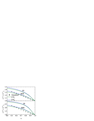
Figure 5: (Color online) Steady-state fourth- and sixth-degree moments, relative to their local equilibrium values, for three-dimensional inelastic hard spheres under uniform shear flow as functions of the coefficient of restitution $\alpha$. The curves are the predictions of the BGK and ES kinetic models with $\beta=\beta_{\eta}$ (dashed lines) and $\beta=\beta_{D}=(1+\alpha)/2$ (solid lines). The circles are simulation results AS05 .

Since the pressure tensor, and hence the reference distribution function $f_{R}$, are entirely known, Eq. (98) gives the explicit solution. From it one can compute any desired velocity moment. Some of those moments are derived in Appendix D. Figure 5 shows $\langle V^{4}\rangle/\langle V^{4}\rangle_{0}$ and $\langle V^{6}\rangle/\langle V^{6}\rangle_{0}$, where $\langle V^{2k}\rangle_{0}=(2T/m)^{k}\Gamma(k+d/2)/\Gamma(d/2)$ is the local equilibrium value, as given by the BGK ($\text{Pr}=1$) and ES ($\text{Pr}=(d-1)/d)$) kinetic models, as well as by Monte Carlo simulations of the Boltzmann equation for IHS AS05 . Even though the ES model is more sophisticated than the BGK model, it gives much poorer predictions for the fourth- and sixth-degree moments than the BGK model. This situation is similar to that found in the elastic case G97 . While this appears as a paradoxical result, one must bear in mind that the real advantage of the ES model over the BGK model occurs when the Prandtl number plays a role, i.e., in states where momentum and energy transfer coexist. Since in the steady uniform shear flow no energy transport is present, there is no reason a priori to expect the ES model to perform better than the BGK model. On the other hand, in the steady Couette flow (where a quasi-parabolic temperature profile coexists with a quasi-linear velocity profile), both models differ already at the level of the non-Newtonian transport properties, the ES model presenting in general a better agreement with simulation results GS03 ; GH97 . In what concerns the influence of $\beta$, we observe in Fig. 5 that $\beta=\beta_{D}=(1+\alpha)/2$ is better for small or moderate inelasticity, while $\beta=\beta_{\eta}$ tends to be better for large inelasticity, an effect that contrasts with that of Fig. 4.

V Concluding remarks

When one aims at understanding the basic properties of fluidized granular media, the prototypical model consists of a system of inelastic hard spheres (IHS) with a constant coefficient of restitution $\alpha$. At a microscopic level of description, kinetic theory has proven to be an efficient tool to unveil some of the most intriguing features of IHS, such as the lack of equilibrium Gibbsian states, high energy overpopulations, clustering instabilities, Maxwell-demon effects, breakdown of energy equipartition, heat fluxes induced by density gradients, segregation in mixtures, phase transitions in velocity space, …The kinetic theory description is based on the Boltzmann and Enskog equations for dilute and dense granular gases, respectively. Both of them assume the molecular chaos hypothesis, according to which the velocities of two particles that are about to collide are uncorrelated. Although the degree of validity of this hypothesis is much more restricted in inelastic collisions than in the case of elastic collisions SPM01 , the Boltzmann and Enskog equations provide useful insights into the peculiar behavior of granular fluids.

Mathematically speaking, the Boltzmann equation for IHS is much more involved than for elastic hard spheres (EHS). As Eqs. (3) and (14) show, the coefficient of restitution $\alpha$ appears inside the velocity integral of the Boltzmann collision operator in a two-fold way. First, it appears explicitly as a factor $\alpha^{-2}$ in front of the gain term as a consequence of the properties $\text{d}\mathbf{v}^{\prime\prime}\text{d}\mathbf{v}_{1}^{\prime\prime}=\alpha^{-1}\text{d}\mathbf{v}\text{d}\mathbf{v}_{1}$ and ${\bf g}^{\prime\prime}\cdot\widehat{\bm{\sigma}}=-\alpha^{-1}{\bf g}\cdot\widehat{\bm{\sigma}}$. Second, the coefficient of restitution appears through the pre-collision velocities $\mathbf{v}^{\prime\prime}$ and $\mathbf{v}_{1}^{\prime\prime}$ given by the collision rule (3). The primary consequence of $\alpha<1$ is the collisional loss of energy, Eqs. (4) and (18), which takes place at a cooling rate $\zeta$ given by Eqs. (19) and (20).

The point we have addressed in this paper is the proposal of a model of granular gases based on the Boltzmann equation for elastic hard spheres (EHS). In this way, the complexities of inelastic collisions for granular kinetic theory are represented by a simple two-fold modification of the more familiar kinetic theory for elastic collisions. Since elastic collisions conserve energy, the fundamental ingredient of the model is the introduction of some kind of external driving that produces a macroscopic cooling effect similar to the one due to inelasticity. While the choice of that driving is not unique, the most intuitive possibility consists of assuming that the EHS gas is under the influence of a (fictitious) drag force $\mathbf{F}_{\text{drag}}=-m\gamma\mathbf{V}$. In order to produce the same cooling effect than in the true IHS gas, the friction constant must be adjusted to be $\gamma=\frac{1}{2}\zeta$. However, since in general $\zeta$ is a complicated nonlinear functional of the one-particle velocity distribution function and we want to keep the frictional EHS model as simple as possible, it is preferable to take $\gamma=\frac{1}{2}\zeta_{0}$, where $\zeta_{0}\propto nT^{1/2}(1-\alpha^{2})$ is the cooling rate in the local equilibrium approximation. The second ingredient of the model is subtler. The application of the drag force is not enough for the EHS gas to mimic, at least quantitatively, some other collisional properties of the IHS gas, apart from the cooling effect. In our model we have assumed that the collisions in the EHS gas are slowed down by a factor $\beta<1$ with respect to the IHS gas. In the dilute limit, this can be interpreted as assuming that the diameter $\sigma^{\prime}$ of EHS is smaller than the diameter $\sigma$ of IHS, namely $\sigma^{\prime}/\sigma=\beta^{1/(d-1)}$. Alternatively, one can interpret $\beta$ as a scaling factor in space and time. Comparison between the Navier–Stokes transport coefficients derived from the Boltzmann equation (in the first Sonine approximation) both for IHS and frictional EHS suggests $\beta=\frac{1}{2}(1+\alpha)$. Moreover, this choice is further supported by the mapping IHS$\to$EHS applied to dilute gas mixtures (see Appendix A) as well as to dense single gases (see Appendix B). In the latter case, due to the physical separation between two colliding particles and the presence of the pair correlation function in the Enskog collision operator, the interpretation of $\beta$ in terms of different sizes $\sigma^{\prime}\neq\sigma$ or as a spatio-temporal scaling factor is not literally correct. In that case, one must understand $\beta$ just as a correction factor modifying the collision rate of EHS relative to that of IHS.

It is obvious that an IHS gas and a gas made of frictional EHS differ in many respects. For instance, the latter admits Maxwellians as uniform solutions (with a time-dependent temperature in the case of the homogeneous cooling state or as a stationary one in the case of a white-noise forcing), while the IHS gas typically exhibits overpopulated high energy tails. However, even though those discrepancies might be qualitatively relevant, they are not quantitatively important in the domain of thermal speeds. In particular, all but the two first distinctive features of granular gases listed in the first paragraph of this Section can be expected to appear in an EHS gas with a state-dependent friction constant $\gamma\propto nT^{1/2}$.

When the gas is in anisotropic and/or inhomogeneous states because of either a transient stage or an instability or the application of boundary conditions, transfers of momentum and/or energy are present, so the velocity distribution function can deviate strongly from a (local) Maxwellian, even for small and moderate velocities. It is in those situations where the frictional EHS gas may be expected to describe the main transport properties of the IHS gas. We have tested this expectation by performing Monte Carlo simulations of the Boltzmann equation under uniform shear flow both for IHS and EHS AS04 ; AS05 . The results show that for moderate inelasticity (say $\alpha=0.9$) one can hardly distinguish the curves representing the transient profiles and the steady-state velocity distribution functions corresponding to both systems. For larger inelasticity (say $\alpha=0.5$) the EHS model still captures almost entirely the nonequilibrium transport properties of the IHS gas.

While the Boltzmann and Enskog equations for the EHS model are mathematically more tractable than those for the true IHS system, their solutions remain a formidable task. In the context of conventional fluids, those difficulties have stimulated the proposal of kinetic models, the prototype of which is the well-known BGK model kinetic equation C88 ; BGK54 . An interesting practical application of the relationship IHS$\leftrightarrow$EHS is the possibility of extending those kinetic models to the case of granular gases in a straightforward way. This has allowed us to recover simplified versions of models previously proposed for dilute and dense single gases BDS99 . In the case of inelastic mixtures, we are not aware of any previous proposal of a kinetic model, despite the fact that several kinetic models exist for elastic mixtures GS03 . Our method permits the construction of extended kinetic models for inelastic mixtures, as will be worked out elsewhere GSD04 .

Appendix A Mixtures

A.1 General properties

In the case of a multi-component granular gas, the inelastic collision between a sphere of species $i$ (mass $m_{i}$ and diameter $\sigma_{i}$) and a sphere of species $j$ (mass $m_{j}$ and diameter $\sigma_{j}$) is characterized by a coefficient of restitution $\alpha_{ij}=\alpha_{ji}$. The direct and restituting collisions rules are given by

$$\begin{array}[]{c}{\bf v}^{\prime}={\bf v}-\mu_{ji}\left(1+\alpha_{ij}\right)({\bf g}\cdot\widehat{\bm{\sigma}})\widehat{\bm{\sigma}},\\ {\bf v}_{1}^{\prime}={\bf v}_{1}+\mu_{ij}\left(1+\alpha_{ij}\right)({\bf g}\cdot\widehat{\bm{\sigma}})\widehat{\bm{\sigma}},\end{array}$$ (101)

$$\begin{array}[]{c}{\bf v}^{\prime\prime}={\bf v}-\mu_{ji}(1+\alpha_{ij}^{-1})({\bf g}\cdot\widehat{\bm{\sigma}})\widehat{\bm{\sigma}},\\ {\bf v}_{1}^{\prime\prime}={\bf v}_{1}+\mu_{ij}(1+\alpha_{ij}^{-1})({\bf g}\cdot\widehat{\bm{\sigma}})\widehat{\bm{\sigma}},\end{array}$$ (102)

where

$$\mu_{ij}\equiv\frac{m_{i}}{m_{i}+m_{j}}.$$ (103)

Equations (101) and (102) are generalizations of Eqs. (1) and (3), respectively. Again, the component of the post-collisional relative velocity along $\widehat{\bm{\sigma}}$ is shrunk by a factor $\alpha_{ij}$, i.e., ${\bf g}^{\prime}\cdot\widehat{\bm{\sigma}}=-\alpha_{ij}{\bf g}\cdot\widehat{\bm{\sigma}}$, and the kinetic energy decreases by a factor proportional to $1-\alpha_{ij}^{2}$, namely

$$m_{i}{v^{\prime}}^{2}+m_{j}{v_{1}^{\prime}}^{2}-m_{i}v^{2}-m_{j}v_{1}^{2}=-({\bf g}\cdot\widehat{\bm{\sigma}})^{2}(1-\alpha_{ij}^{2})\frac{m_{i}m_{j}}{m_{i}+m_{j}}.$$ (104)

From the velocity distribution function $f_{i}(\mathbf{v})$ of species $i$ one can define the number density

$$n_{i}=\int\text{d}\mathbf{v}\,f_{i}(\mathbf{v}),$$ (105)

the mass density $\rho_{i}=m_{i}n_{i}$, and the average velocity

$$\mathbf{u}_{i}=\frac{1}{n_{i}}\int\text{d}\mathbf{v}\,\mathbf{v}f_{i}(\mathbf{v})$$ (106)

of species $i$. The associated global quantities are the total number density $n=\sum_{i}n_{i}$, the total mass density $\rho=\sum_{i}\rho_{i}$, and the (barycentric) flow velocity

$$\mathbf{u}=\frac{1}{\rho}\sum_{i}\rho_{i}\mathbf{u}_{i}.$$ (107)

The granular temperature $T$ of the mixture is defined by

$$T=\frac{1}{n}\sum_{i}n_{i}T_{i},\quad\frac{d}{2}n_{i}T_{i}=\frac{m_{i}}{2}\int\text{d}\mathbf{v}\,V^{2}f_{i}(\mathbf{v}),$$ (108)

where $\mathbf{V}=\mathbf{v}-\mathbf{u}$ is the peculiar velocity. In Eq. (108) $T_{i}$ is the partial granular temperature associated with species $i$. In general, equipartition of energy does not hold, even in homogeneous states, so $T_{i}\neq T$ GD99 .

In the dilute limit, the distribution functions $f_{i}(\mathbf{v})$ obey a set of coupled Boltzmann equations,

$$\left(\partial_{t}+\mathbf{v}\cdot\nabla\right)f_{i}=\sum_{j}J_{ij}^{(\alpha_{ij})}[f_{i},f_{j}],$$ (109)

where the collision operator $J_{ij}^{(\alpha_{ij})}[f_{i},f_{j}]$ is given by

$$J_{ij}^{(\alpha_{ij})}[f_{i},f_{j}]=\sigma_{ij}^{d-1}\int\text{d}{\bf v}_{1}\int\text{d}\widehat{\bm{\sigma}}\,\Theta({\bf g}\cdot\widehat{\bm{\sigma}})({\bf g}\cdot\widehat{\bm{\sigma}})$$

$$\times\left[\alpha_{ij}^{-2}f_{i}({\bf v}^{\prime\prime})f_{j}({\bf v}_{1}^{\prime\prime})-f_{i}({\bf v})f_{j}({\bf v}_{1})\right],$$ (110)

where $\sigma_{ij}\equiv(\sigma_{i}+\sigma_{j})/2$. Every collision conserves the number of particles of each species,

$$\int\text{d}\mathbf{v}\,J_{ij}^{(\alpha_{ij})}[f_{i},f_{j}]=0.$$ (111)

Moreover, the total momentum is conserved as well, i.e.,

$$\sum_{i,j}m_{i}\int\text{d}\mathbf{v}\,\mathbf{v}J_{ij}^{(\alpha_{ij})}[f_{i},f_{j}]=\mathbf{0}.$$ (112)

However, the total energy is not conserved:

$$\sum_{i,j}\frac{m_{i}}{2}\int\text{d}\mathbf{v}\,V^{2}J_{ij}^{(\alpha_{ij})}[f_{i},f_{j}]=-\frac{d}{2}nT\zeta,$$ (113)

what defines the collision rate $\zeta$ of the mixture.

In general, given an arbitrary function $\phi(\mathbf{v})$, one can define its associated collision integral

$$I_{ij}^{(\alpha_{ij})}[\phi] \equiv \int\text{d}\mathbf{v}\phi(\mathbf{v})J_{ij}^{(\alpha_{ij})}[f_{i},f_{j}]$$ (114)

$$= \sigma_{ij}^{d-1}\int\text{d}\mathbf{v}\int\text{d}{\bf v}_{1}\int\text{d}\widehat{\bm{\sigma}}\,\Theta({\bf g}\cdot\widehat{\bm{\sigma}})({\bf g}\cdot\widehat{\bm{\sigma}})$$

$$\times f_{i}({\bf v})f_{j}({\bf v}_{1})\left[\phi(\mathbf{v}^{\prime})-\phi(\mathbf{v})\right],$$

where in the last step we have performed a standard change of variables. Thus, Eqs. (111)–(113) can be rewritten as

$$I_{ij}^{(\alpha_{ij})}[1]=0,$$ (115)

$$\sum_{i,j}I_{ij}^{(\alpha_{ij})}[m_{i}\mathbf{v}]=\mathbf{0},$$ (116)

$$\zeta=-\frac{1}{dnT}\sum_{i,j}I_{ij}^{(\alpha_{ij})}[m_{i}V^{2}].$$ (117)

The collision integrals $I_{ij}^{(\alpha_{ij})}[m_{i}\mathbf{v}]$ and $I_{ij}^{(\alpha_{ij})}[m_{i}V^{2}]$ cannot be evaluated exactly for arbitrary distribution functions $f_{i}$ and $f_{j}$. This situation is analogous to the one taking place with Eq. (20) in the single gas case. Again, a reasonable estimate can be expected if the integrals are evaluated in the (multi-temperature) Gaussian approximation

$$f_{i}(\mathbf{v})\to f_{i,0}(\mathbf{v})=n_{i}\left(\frac{m_{i}}{2\pi T_{i}}\right)^{d/2}\exp\left(-m_{i}V^{2}/2T_{i}\right),$$ (118)

where we have restricted ourselves to the case $\mathbf{u}_{i}=\mathbf{u}$ in order to satisfy Eq. (106). When the approximation (118) is inserted into Eq. (114) one gets GD02 ; GM03

$$I_{ij}^{(\alpha_{ij})}[m_{i}\mathbf{v}]\to 0,$$ (119)

$$I_{ij}^{(\alpha_{ij})}[m_{i}V^{2}] \to (d+2)n_{i}T_{i}\nu_{ij}\frac{1+\alpha_{ij}}{2}$$ (120)

$$\times\left[\frac{m_{i}(T_{j}-T_{i})}{m_{j}T_{i}+m_{i}T_{j}}-\frac{1-\alpha_{ij}}{2}\right],$$

where

$$\nu_{ij}=\frac{4\Omega_{d}}{\sqrt{\pi}(d+2)}n_{j}\mu_{ji}^{2}\sigma_{ij}^{d-1}\left(\frac{2T_{i}}{m_{i}}\right)^{1/2}\left(1+\frac{m_{i}T_{j}}{m_{j}T_{i}}\right)^{3/2}$$ (121)

is an effective collision frequency of a particle of species $i$ with particles of species $j$. In this Gaussian approximation, the cooling rate defined by Eq. (117) becomes $\zeta\to\zeta_{0}$ with

$$\zeta_{0}=\frac{d+2}{4dnT}\sum_{i,j}n_{i}T_{i}\nu_{ij}\left(1-\alpha_{ij}^{2}\right),$$ (122)

where we have made use of the property $\rho_{i}T_{i}\nu_{ij}=\rho_{j}T_{j}\nu_{ji}$. In the case of a single gas, Eqs. (121) and (122) reduce to Eqs. (26) and (25), respectively.

A.2 Model of frictional elastic hard spheres

Once we have revised some of the basic properties of the collision operator $J_{ij}^{(\alpha_{ij})}[f_{i},f_{j}]$ for an IHS mixture, we are in conditions of proposing a minimal model for frictional EHS. In agreement with the philosophy behind Eq. (31), we write

$$J_{ij}^{(\alpha_{ij})}[f_{i},f_{j}]\to\beta_{ij}J_{ij}^{(1)}[f_{i},f_{j}]+\frac{\zeta_{ij}}{2}\frac{\partial}{\partial{\bf v}}\cdot\left[\left({\bf v}-\mathbf{u}_{i}\right)f_{i}\right],$$ (123)

where $\beta_{ij}$ and $\zeta_{ij}$ are to be determined by optimizing the agreement between the relevant properties of the true operator $J_{ij}^{(\alpha_{ij})}[f_{i},f_{j}]$ and those of the right-hand side of Eq. (123). For an arbitrary function $\phi(\mathbf{v})$, one has

$$I_{ij}^{(\alpha_{ij})}[\phi]\to\beta_{ij}I_{ij}^{(1)}[\phi]-\frac{\zeta_{ij}}{2}\int\text{d}\mathbf{v}\left({\bf v}-\mathbf{u}_{i}\right)\cdot\frac{\partial\phi(\mathbf{v})}{\partial{\bf v}}f_{i}(\mathbf{v}).$$ (124)

The above replacement satisfies Eq. (115) identically. In addition, it is consistent with Eq. (119) in the Gaussian approximation (118). So far, $\beta_{ij}$ and $\zeta_{ij}$ remain arbitrary. Insertion of the Gaussian approximation (118) into Eq. (124) with $\phi(\mathbf{v})=m_{i}V^{2}$ yields

$$I_{ij}^{(\alpha_{ij})}[m_{i}V^{2}] \to \beta_{ij}(d+2)n_{i}T_{i}\nu_{ij}\frac{m_{i}(T_{j}-T_{i})}{m_{j}T_{i}+m_{i}T_{j}}$$ (125)

$$-\zeta_{ij}dn_{i}T_{i},$$

where again we have restricted ourselves to the case $\mathbf{u}_{i}=\mathbf{u}$. Comparison between Eqs. (120) and (125) suggests the choices

$$\beta_{ij}=\frac{1+\alpha_{ij}}{2},$$ (126)

$$\zeta_{ij}=\frac{d+2}{4d}\nu_{ij}\left(1-\alpha_{ij}^{2}\right).$$ (127)

Of course, other combinations of $\beta_{ij}$ and $\zeta_{ij}$ are in principle possible, but Eqs. (126) and (127) represent the simplest choice in the absence of mutual diffusion (i.e., with $\mathbf{u}_{i}=\mathbf{u}$). In the more general case $\mathbf{u}_{i}\neq\mathbf{u}$, the expression for $\zeta_{ij}$ is more complicated and will be reported elsewhere GSD04 .

Equation (125) highlights that in general $I^{(\alpha_{ij})}[m_{i}V^{2}]\neq 0$ because of two reasons. First, if species $i$ and $j$ have different mean kinetic energies (i.e., $T_{i}\neq T_{j}$), then mutual collisions tend to “equilibrate” both partial temperatures. This equipartition effect, which is also present in the case of elastic collisions, is represented by the term $\beta_{ij}I^{(1)}[m_{i}V^{2}]$. Moreover, even if $T_{i}=T_{j}$, one has $I^{(\alpha_{ij})}[m_{i}V^{2}]\neq 0$ due to the inelasticity of collisions, an effect that is accounted for by the term $-\zeta_{ij}dn_{i}T_{i}$. While the former term can be either positive ($T_{i}<T_{j}$) or negative ($T_{i}>T_{j}$), the latter term is negative definite. Thus, $\zeta_{ij}$ represents the cooling rate of species $i$ due to collisions with particles of species $j$. Since the relative decrease of energy after each $i$-$j$ collision is proportional to $1-\alpha_{ij}^{2}$, it is quite natural that $\zeta_{ij}\propto 1-\alpha_{ij}^{2}$. As in the single gas case, the parameter $\beta_{ij}$ measures the rate of $i$-$j$ collisions of EHS relative to that of IHS. It is rather reinforcing that the choice (126) is the natural extension of the choice (65) that we adopted for a single gas. While in the latter case we had to resort to the evaluation of the transport coefficients, the choice (126) arises in the case of mixtures simply from the collisional energy transfer when $T_{i}\neq T_{j}$.

A.3 Brownian limit

Let us consider now the Brownian limit of a heavy impurity particle (species 1) immersed in a bath of light particles (species 2). In that case, the Boltzmann–Lorentz operator for inelastic collisions becomes the Fokker–Planck operator BDS99

$$J_{12}^{(\alpha_{12})}[f_{1},f_{2}]=\frac{1+\alpha_{12}}{2}J_{12}^{(1)}[f_{1},f_{2}]-\frac{1}{2}\zeta_{12}\frac{T_{1}}{m_{1}}\frac{\partial^{2}}{\partial v^{2}}f_{1},$$ (128)

where

$$J_{12}^{(1)}[f_{1},f_{2}]=\gamma_{12}\frac{\partial}{\partial\mathbf{v}}\cdot\left(\mathbf{v}+\frac{T_{2}}{m_{1}}\frac{\partial}{\partial\mathbf{v}}\right)f_{1}.$$ (129)

In the above equations,

$$\gamma_{12}=\frac{2\Omega_{d}}{d\sqrt{\pi}}n_{2}\sigma_{12}^{(d-1}(m_{2}/m_{1})^{1/2}\left(\frac{2T_{2}}{m_{1}}\right)^{1/2}$$ (130)

is the friction constant associated with elastic collisions and

$$\zeta_{12}=\frac{\gamma_{12}}{2}\frac{T_{2}}{T_{1}}(1-\alpha_{12}^{2})$$ (131)

is the cooling rate of the Brownian particle due to inelastic collisions with the bath particles. Equation (128) is the exact Fokker–Plank limit of the inelastic Boltzmann–Lorentz operator. It is quite nice that Eq. (128) supports the choice (126) as the collision rate factor. Moreover, Eq. (131) for $\zeta_{12}$ agrees with the limit $m_{1}\gg m_{2}$ of the proposal (127). On the other hand, the exact Fokker–Planck equation (128) differs from the one obtained from our model (123). More specifically, the latter results from the replacement

$$-\frac{\zeta_{12}}{2}\frac{T_{1}}{m_{1}}\frac{\partial^{2}}{\partial v^{2}}f_{1}\to\frac{\zeta_{12}}{2}\frac{\partial}{\partial{\bf v}}\cdot\left[({\bf v}-{\bf u}_{1})f_{1}\right].$$ (132)

While on the right-hand side of (132) the role of mimicking the collisional cooling experienced by the Brownian particle is played by a deterministic frictional force, that role is played by a stochastic force on the left-hand side. On the other hand, both sides of (132) agree in that they give vanishing contributions to the mass and momentum balance equations and yield the same contribution to the energy balance equation if $\mathbf{u}_{1}=\mathbf{u}$. In addition, they coincide in the Gaussian approximation (118). Therefore, the model (123) can be expected to behave reasonably well even in the extreme limit of a Brownian particle.

A.4 Kinetic modeling

As discussed in Sec. IV, the mapping (123) allows one to transfer any given kinetic model

$$J_{ij}^{(1)}[f_{i},f_{j}]\to K_{ij}^{(1)}$$ (133)

for elastic mixtures GS03 into an equivalent model for inelastic mixtures:

$$J_{ij}^{(\alpha_{ij})}[f_{i},f_{j}]\to K_{ij}^{(\alpha_{ij})}=\beta_{ij}K_{ij}^{(1)}+\frac{\zeta_{ij}}{2}\frac{\partial}{\partial{\bf v}}\cdot\left[\left({\bf v}-\mathbf{u}_{i}\right)f_{i}\right].$$ (134)

Thus, one can construct in a straightforward way the inelastic versions of kinetic models such as Gross–Krook’s GK56 , Garzó–Santos–Brey’s GSB89 , or Andries–Aoki–Perthame’s AAP02 . More details will be reported elsewhere GSD04 .

Appendix B Dense granular gases

B.1 The Enskog equation for inelastic hard spheres

So far, we have restricted ourselves to low density granular gases for which the Boltzmann description seems appropriate. At higher densities the revised Enskog kinetic theory, suitably generalized to inelastic collisions BDS97 , provides a basis for analysis of granular flow. The Enskog kinetic equation reads

$$\left(\partial_{t}+{\bf v\cdot\nabla}\right)f=J_{E}^{(\alpha)}[f],$$ (135)

where

$$J_{E}^{(\alpha)}[f]=\sigma^{d-1}\int\text{d}{\bf v}_{1}\int\text{d}\widehat{\bm{\sigma}}\,\Theta({\bf g}\cdot\widehat{\bm{\sigma}})({\bf g}\cdot\widehat{\bm{\sigma}})$$

$$\times\left[\alpha^{-2}f_{2}({\bf r},{\bf r}-{\bm{\sigma}},{\bf v}^{\prime\prime},{\bf v}^{\prime\prime}_{1})-f_{2}({\bf r},{\bf r}+{\bm{\sigma}},{\bf v},{\bf v}_{1})\right].$$ (136)

In this equation, $\bm{\sigma}\equiv\sigma\widehat{\bm{\sigma}}$ and

$$f_{2}(\mathbf{r},\mathbf{r}\pm{\bm{\sigma}},\mathbf{v},\mathbf{v}_{1})=\chi(\mathbf{r},\mathbf{r}\pm{\bm{\sigma}})f(\mathbf{r},\mathbf{v})f(\mathbf{r}\pm{\bm{\sigma}},\mathbf{v}_{1})$$ (137)

is the pre-collisional two-body distribution function in the molecular chaos approximation, $\chi(\mathbf{r},\mathbf{r}\pm{\bm{\sigma}})$ being the equilibrium pair correlation function at contact as a functional of the density field. We use the notation $J_{E}^{(\alpha)}[f]$ rather than $J_{E}^{(\alpha)}[f,f]$ to remind that the nonlinear functional dependence of the Enskog collision operator on the velocity distribution function $f$ is higher than bilinear, due to the presence of the correlation function $\chi$.

Taking velocity moments in (135) one obtains again the hydrodynamic balance equations (6)–(8), where the number density, flow velocity, and granular temperature are defined by Eqs. (15)–(17), respectively. The pressure tensor and the heat flux have both kinetic and collisional transfer contributions, namely $\mathsf{P}=\mathsf{P}_{k}+\mathsf{P}_{c}$, $\mathbf{q}=\mathbf{q}_{k}+\mathbf{q}_{c}$. The kinetic contributions $\mathsf{P}_{k}$ and $\mathbf{q}_{k}$ are given by Eqs. (21) and (22), while the collisional transfer parts are BDS97

$$\mathsf{P}_{c}^{(\alpha)}[f] = \frac{1+\alpha}{4}m\sigma^{d}\int\text{d}\mathbf{v}\int\text{d}{\bf v}_{1}\int\text{d}\widehat{\bm{\sigma}}\,\Theta({\bf g}\cdot\widehat{\bm{\sigma}})({\bf g}\cdot\widehat{\bm{\sigma}})^{2}$$

$$\times\widehat{\bm{\sigma}}\widehat{\bm{\sigma}}\int_{0}^{1}\text{d}\lambda\,f_{2}\left({\bf r}-(1-\lambda){\bm{\sigma}},{\bf r}+\lambda{\bm{\sigma}},{\bf v},{\bf v}_{1}\right),$$

$$\mathbf{q}_{c}^{(\alpha)}[f] = \frac{1+\alpha}{4}m\sigma^{d}\int\text{d}\mathbf{v}\int\text{d}{\bf v}_{1}\int\text{d}\widehat{\bm{\sigma}}\,\Theta({\bf g}\cdot\widehat{\bm{\sigma}})({\bf g}\cdot\widehat{\bm{\sigma}})^{2}$$

$$\times(\mathbf{G}\cdot\widehat{\bm{\sigma}})\widehat{\bm{\sigma}}\int_{0}^{1}\text{d}\lambda\,f_{2}({\bf r}-(1-\lambda){\bm{\sigma}},{\bf r}+\lambda{\bm{\sigma}},{\bf v},{\bf v}_{1}),$$

where $\mathbf{G}\equiv(\mathbf{V}+\mathbf{V}_{1})/2=(\mathbf{v}+\mathbf{v}_{1})/2-\mathbf{u}(\mathbf{r})$. The superscript $(\alpha)$ on $\mathsf{P}_{c}^{(\alpha)}$ and $\mathbf{q}_{c}^{(\alpha)}$ has been introduced to emphasize that both quantities depend explicitly on the coefficient of restitution. They also depend implicitly on $\alpha$ through their functional dependence on the velocity distribution function $f$. With that convention, we can write

$$\mathsf{P}_{c}^{(\alpha)}[f]=\frac{1+\alpha}{2}\mathsf{P}_{c}^{(1)}[f],\quad\mathbf{q}_{c}^{(\alpha)}[f]=\frac{1+\alpha}{2}\mathbf{q}_{c}^{(1)}[f].$$ (140)

The cooling rate is found to be BDS97 ; BDS99

$$\zeta = (1-\alpha^{2})\frac{m\sigma^{d-1}}{4dnT}\int\text{d}\mathbf{v}\int\text{d}{\bf v}_{1}\int\text{d}\widehat{\bm{\sigma}}\,\Theta({\bf g}\cdot\widehat{\bm{\sigma}})({\bf g}\cdot\widehat{\bm{\sigma}})^{3}$$ (141)

$$\times f_{2}({\bf r},{\bf r}+{\bm{\sigma}},{\bf v},{\bf v}_{1}).$$

The divergences of the collisional transfer parts are simply related to moments of the collision operator BDS97 ,

$$\nabla\cdot\mathsf{P}_{c}^{(\alpha)}=-m\int\text{d}\mathbf{V}\,\mathbf{V}J^{(\alpha)}_{E}[f],$$ (142)

$$\nabla\cdot\mathbf{q}_{c}^{(\alpha)}=-\frac{m}{2}\int\text{d}\mathbf{V}\,{V^{2}}J^{(\alpha)}_{E}[f]-\mathsf{P}_{c}^{(\alpha)}:\nabla\mathbf{u}-\frac{d}{2}n\zeta T.$$ (143)

As in the dilute case, a reasonable estimate of the cooling rate $\zeta(\mathbf{r},t)$ can be expected if the velocity distribution function is replaced by its local equilibrium approximation (23). The resulting cooling rate is

$$\zeta_{0}(\mathbf{r}) = (1-\alpha^{2})\frac{m\sigma^{d-1}}{4\pi^{d}dT(\mathbf{r})}\int\text{d}\mathbf{C}\int\text{d}\mathbf{C}_{1}\text{$e$}^{-C^{2}-C_{1}^{2}}$$

$$\times\int\text{d}\widehat{\bm{\sigma}}\,\Theta({\bf g}\cdot\widehat{\bm{\sigma}})({\bf g}\cdot\widehat{\bm{\sigma}})^{3}\chi(\mathbf{r},\mathbf{r}+\bm{\sigma})n(\mathbf{r}+\bm{\sigma}),$$

(144)

where now $\mathbf{g}=\sqrt{2T(\mathbf{r})/m}\mathbf{C}-\sqrt{2T(\mathbf{r}+\bm{\sigma})/m}\mathbf{C}_{1}+\mathbf{u}(\mathbf{r})-\mathbf{u}(\mathbf{r}+\bm{\sigma})$. The local equilibrium cooling rate $\zeta_{0}(\mathbf{r})$ depends not only on the local values of the hydrodynamic fields at $\mathbf{r}$ but also on their values on a spherical surface of radius $\sigma$ around the point $\mathbf{r}$. It also depends on the entire density field through $\chi(\mathbf{r},\mathbf{r}+\bm{\sigma})$. If one further neglects those dependencies, one gets the same result as in the dilute limit, Eqs. (25) and (26), except that the collision frequency $\nu_{0}$ is multiplied by $\chi$.

B.2 Model of frictional elastic hard spheres

The natural extension to the Enskog equation of the model (31) is

$$J_{E}^{(\alpha)}[f]\to\beta J^{(1)}_{E}[f]+\frac{\zeta_{0}}{2}\frac{\partial}{\partial{\bf v}}\cdot\left({\bf V}f\right).$$ (145)

Insertion of (145) into Eqs. (142) and (143) yields

$$\nabla\cdot\mathsf{P}_{c}^{(\alpha)}\to\beta\nabla\cdot\mathsf{P}_{c}^{(1)},$$ (146)

$$\nabla\cdot\mathbf{q}_{c}^{(\alpha)}+\mathsf{P}_{c}^{(\alpha)}:\nabla\mathbf{u}\to\beta\left[\nabla\cdot\mathbf{q}_{c}^{(1)}+\mathsf{P}_{c}^{(1)}:\nabla\mathbf{u}\right],$$ (147)

where in Eq. (147) we have approximated $\zeta\to\zeta_{0}$. Comparison with the exact results (140) implies that $\beta=(1+\alpha)/2$. Again, this reinforces the choice (65) made in the dilute case.

B.3 Kinetic modeling

A few years ago, Dufty et al. DSB96 ; SMDB98 proposed the following BGK-like kinetic model for the elastic Enskog equation:

$$J_{E}^{(1)}[f] \to -\nu_{0}\left(f-f_{0}\right)-\frac{f_{0}}{nT}\left[\mathbf{V}\nabla:\mathsf{P}_{c}^{(1)}\right.$$ (148)

$$+\left(\frac{mV^{2}}{dT}-1\right)\left(\nabla\cdot\mathbf{q}_{c}^{(1)}+\mathsf{P}_{c}^{(1)}:\nabla\mathbf{u}\right)$$

$$\left.-\mathsf{A}^{(1)}:\mathsf{D}(\mathbf{V})-\mathbf{B}^{(1)}\cdot\mathbf{S}(\mathbf{V})\right],$$

where

$$\mathsf{A}^{(1)}\equiv\frac{1}{2T}\int\text{d}\mathbf{v}\,\mathsf{D}(\mathbf{V})J_{E}^{(1)}[f_{0}],$$ (149)

$$\mathbf{B}^{(1)}\equiv\frac{2m}{(d+2)T^{2}}\int\text{d}\mathbf{v}\,\mathbf{S}(\mathbf{V})J_{E}^{(1)}[f_{0}].$$ (150)

In Eqs. (148)–(150), $\mathsf{D}(\mathbf{V})$ and $\mathbf{S}(\mathbf{V})$ are given by Eqs. (43) and (45), respectively. Now, making use of (145), the kinetic model (148) is extended to inelastic collisions as

$$J_{E}^{(\alpha)}[f] \to -\frac{1+\alpha}{2}\nu_{0}\left(f-f_{0}\right)+\frac{\zeta_{0}}{2}\frac{\partial}{\partial\mathbf{v}}\cdot\left(\mathbf{V}f\right)$$ (151)

$$-\frac{f_{0}}{nT}\left[\mathbf{V}\nabla:\mathsf{P}_{c}^{(\alpha)}+\left(\frac{mV^{2}}{dT}-1\right)\right.$$

$$\times\left(\nabla\cdot\mathbf{q}_{c}^{(\alpha)}+\mathsf{P}_{c}^{(\alpha)}:\nabla\mathbf{u}\right)$$

$$\left.-\mathsf{A}^{(\alpha)}:\mathsf{D}(\mathbf{V})-\mathbf{B}^{(\alpha)}\cdot\mathbf{S}(\mathbf{V})\right],$$

where $\mathsf{A}^{(\alpha)}=\frac{1}{2}(1+\alpha)\mathsf{A}^{(1)}$, $\mathbf{B}^{(\alpha)}=\frac{1}{2}(1+\alpha)\mathbf{B}^{(1)}$. The kinetic model (151) for the inelastic Enskog equation turns out to be a simplified version of the model introduced in Ref. BDS99 .

Appendix C Inelastic Maxwell models

C.1 Transport coefficients

Now we return to a single dilute gas. In principle, the same philosophy behind Eq. (31) can be applied to inelastic Maxwell models (IMM). In that case, the collision operator is S03 ; EB02

$$J^{(\alpha)}[f,f]=\frac{(d+2)\nu_{0}}{2n\Omega_{d}}\int\text{d}{\bf v}_{1}\int\text{d}\widehat{\bm{\sigma}}\,\left[\alpha^{-1}f({\bf r},{\bf v}^{\prime\prime})\right.$$

$$\left.\times f({\bf r},{\bf v}_{1}^{\prime\prime})-f({\bf r},{\bf v})f({\bf r},{\bf v}_{1})\right].$$ (152)

This collision operator verifies again Eq. (18) but now the cooling rate is exactly given by $\zeta=\zeta_{0}$, Eq. (25). The transport coefficients associated with the stress tensor and the heat flux have the structure of Eqs. (37)–(39), except that now the collision frequencies are S03

$$\nu_{\eta}^{*}=\frac{(1+\alpha)(d+1-\alpha)}{2d}$$ (153)

$$\nu_{\lambda}^{*}=\frac{1+\alpha}{d}\left[\frac{d-1}{2}+\frac{1}{8}(d+8)(1-\alpha)\right],$$ (154)

and the kurtosis of the homogeneous cooling state is

$$a_{2}^{\text{hc}}=\frac{6(1-\alpha)^{2}}{4d-7+3\alpha(2-\alpha)}.$$ (155)

Using the property G03b

$$\int\text{d}\mathbf{v}\,\mathbf{v}J^{(\alpha)}[f_{\text{t}},f_{\text{hc}}]=-\frac{d+2}{2d}\nu_{0}\mathbf{j}_{\text{t}}$$ (156)

it is straightforward to prove that the self-diffusion coefficient is given by Eq. (59), except that

$$\nu_{D}^{*}=\frac{d+2}{2d}\frac{1+\alpha}{2}.$$ (157)

The Navier–Stokes transport coefficients characterizing an IMM mixture have been recently derived GA04 .

C.2 Model of frictional elastic Maxwell particles

In the case of frictional elastic Maxwell models (EMM), one makes the replacement (31). The corresponding transport coefficients have the same forms as for EHS, so they are given again by Eqs. (51)–(53) and (64). In the same spirit as before, if we want to optimize the agreement between the EMM and IMM transport coefficients, the three possible choices for $\beta$ are

$$\beta_{\eta}=\nu_{\eta}^{*}-\zeta_{0}^{*}=\frac{(1+\alpha)^{2}}{4},$$ (158)

$$\beta_{\lambda}=\frac{d}{d-1}\left(\nu_{\lambda}^{*}-\frac{3}{2}\zeta_{0}^{*}\right)=\frac{(1+\alpha)^{2}}{4},$$ (159)

$$\beta_{D}=\frac{2d}{d+2}\nu_{D}^{*}=\frac{1+\alpha}{2}.$$ (160)

Interestingly, the shear viscosity and the thermal conductivity routes give consistently the same expression for $\beta$, this expression being the square of the self-diffusion value. Since $a_{2}^{\text{hc}}$, which vanishes for EMM, does not appear either in the shear viscosity or in the self-diffusion coefficient of IMM, the EMM model reproduces exactly those coefficients if $\beta=\beta_{\eta}=(1+\alpha)^{2}/4$ and $\beta=\beta_{D}=(1+\alpha)/2$, respectively. However, even if $\beta=\beta_{\lambda}=(1+\alpha)^{2}/4$, the transport coefficients $\lambda$ and $\mu$ for IMM differ from those for EMM due to the explicitly appearance of $a_{2}^{\text{hc}}$ in the former case.

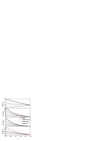
Figure 6: (Color online) Plot of the (reduced) shear viscosity $\eta/(nT/\nu_{0})$, thermal conductivity $\lambda/(nT/m\nu_{0})$, transport coefficient $\mu/(T^{2}/m\nu_{0})$, and self-diffusion coefficient $D/(T/m\nu_{0})$ for three-dimensional IMM (—) and the “equivalent” system of EMM with $\beta=\beta_{\eta}=\beta_{\lambda}$ (– – –), $\beta=\beta_{D}$ (– $\cdot$ – $\cdot$ –), and $\beta=1$ (– $\cdot\cdot$ – $\cdot\cdot$ –) as functions of the coefficient of restitution $\alpha$. Note that in the top panel the IHS curve and the EHS curve with $\beta=\beta_{\eta}=\beta_{\lambda}$ are identical. The same happens in the bottom panel between the IHS curve and the EHS curve with $\beta=\beta_{D}$.

As Fig. 6 shows, the choice $\beta=\beta_{D}=(1+\alpha)/2$ describes the behavior of $\eta$, $\lambda$, and $\mu$ only at a rough qualitative level. The alternative choice $\beta=\beta_{\eta}=\beta_{\lambda}=(1+\alpha)^{2}/4$ strongly overestimates the diffusion coefficient and gives values for $\lambda$ and $\mu$ in reasonable agreement with the true IMM values only for small or moderate inelasticity. Therefore, the Navier–Stokes transport coefficients of IMM are very poorly described by the EMM model with a unique expression for $\beta$, in contrast to what happens in the case $\text{IHS}\leftrightarrow\text{EHS}$. This a consequence of the fact that the influence of inelasticity is much stronger in IMM than in IHS, as reflected on the kurtosis $a_{2}^{\text{hc}}$ and on the transport coefficients $\eta$, $\lambda$, $\mu$, and $D$ (compare Figs. 3 and 6). As a matter of fact, the coefficients $\lambda$ and $\mu$ diverge at $\alpha=(4-d)/3d$ for $d=2$ and $d=3$ S03 , thus indicating the failure of a hydrodynamic description for IMM with $\alpha\leq(4-d)/3d$.

While, with the exception of the self-diffusion coefficient GA04 , the Navier–Stokes transport coefficients of IHS and IMM differ significantly S03 , those of frictional EHS and EMM agree each other [see Eqs. (51)–(53) and (64)], provided the former are evaluated in the first Sonine approximation and the same value of $\beta$ is used in both approaches. As a matter of fact, hard spheres and Maxwell particles are known to exhibit similar rheological properties in the elastic case, even in states far from equilibrium GS03 . This shows that the EMM system with $\beta=(1+\alpha)/2$ can be usefully exploited as a model of IHS rather than as a model of IMM, namely

$$J_{\text{IHS}}^{(\alpha)}[f,f]\to\frac{1+\alpha}{2}J_{\text{EMM}}^{(1)}[f,f]+\frac{\zeta_{0}}{2}\frac{\partial}{\partial\mathbf{v}}\cdot\left(\mathbf{V}f\right).$$ (161)

Since the collision operator of EMM is mathematically more tractable than that of EHS, the mapping $\text{IHS}\to\text{EMM}$ can be considered as intermediate between the mappings $\text{IHS}\to\text{EHS}$ and $\text{IHS}\to\text{kinetic models}$.

Appendix D Velocity moments in the uniform shear flow

In this Appendix we derive some expressions for the velocity moments predicted by the BGK and ES kinetic models for uniform shear flow. Let us focus on the isotropic moments

$$\langle V^{2N}\rangle=\frac{1}{n}\int\text{d}\mathbf{V}V^{2N}f(\mathbf{V}).$$ (162)

Insertion of the steady-state solution (98) yields

$$\langle V^{2N}\rangle = \frac{\beta\nu_{0}\text{Pr}}{n}\int_{0}^{\infty}\text{d}s\,\exp\left[-\left(\beta\nu_{0}\text{Pr}+{N}\zeta_{0}\right)s\right]$$ (163)

$$\times\int\text{d}\mathbf{V}f_{R}\left(\mathbf{V}\right)|\mathsf{A}(s)\cdot\mathbf{V}|^{2N},$$

where $A_{ij}(s)=\delta_{ij}-as\delta_{ix}\delta_{jy}$. To carry out the velocity integral, we consider the diagonal representation of the matrix $\mathsf{R}^{-1}$, namely

$$\mathsf{S}=\frac{mn}{2}\mathsf{U}\cdot\mathsf{R}^{-1}\cdot\mathsf{U}^{-1},$$ (164)

where $\mathsf{U}$ is a unitary matrix whose expression will be omitted here. The eigenvalues are

$$S_{1,2}=\frac{m}{2T}\frac{2\text{Pr}(\beta+\zeta_{0}^{*})}{2(\text{Pr}\beta+\zeta_{0}^{*})\pm(1-\text{Pr})\left[\sqrt{d\zeta_{0}^{*}(2\beta+d\zeta_{0}^{*})}\mp d\zeta_{0}\right]},$$ (165)

$$S_{3}=\frac{m}{2T}\frac{\text{Pr}(\beta+\zeta_{0}^{*})}{\text{Pr}\beta+\zeta_{0}^{*}},$$ (166)

where $S_{3}$ is $(d-2)$-fold degenerate.

Using (164), the velocity integral in Eq. (163) becomes

$$\int\text{d}\mathbf{V}f_{R}\left(\mathbf{V}\right)|\mathsf{A}(s)\cdot\mathbf{V}|^{2N}=n\pi^{-d/2}\left(\det\mathsf{S}\right)^{1/2}$$

$$\times\int\text{d}\mathbf{W}\text{$e$}^{-\mathsf{S}:\mathbf{W}\mathbf{W}}|\mathsf{A}(s)\cdot\mathsf{U}^{-1}\cdot\mathbf{W}|^{2N},$$ (167)

where we have made the change of variables

$$\mathbf{V}\to\mathbf{W}=\mathsf{U}\cdot\mathbf{V}.$$ (168)

It is convenient to decompose the vector $\mathbf{W}$ as

$$\mathbf{W}=W_{x}\widehat{\mathbf{x}}+W_{y}\widehat{\mathbf{y}}+\mathbf{W}_{\perp},$$ (169)

so that

$$|\mathsf{A}(s)\cdot\mathsf{U}^{-1}\cdot\mathbf{W}|^{2} = W_{\perp}^{2}+B_{xx}(s)W_{x}^{2}+2B_{xy}(s)W_{x}W_{y}$$ (170)

$$+B_{yy}(s)W_{y}^{2},$$

where

$$B_{xx}(s)=1+\frac{1}{2}a^{2}s^{2}-as\frac{\sqrt{2\beta}+as\sqrt{d\zeta_{0}^{*}}/2}{\sqrt{2\beta+d{\zeta_{0}^{*}}}},$$ (171)

$$B_{yy}(s)=1+\frac{1}{2}a^{2}s^{2}+as\frac{\sqrt{2\beta}-as\sqrt{d\zeta_{0}^{*}}/2}{\sqrt{2\beta+d{\zeta_{0}^{*}}}},$$ (172)

$$B_{xy}(s)=as\frac{as\sqrt{\beta/2}+\sqrt{d\zeta_{0}^{*}}}{\sqrt{2\beta+d\zeta_{0}^{*}}}.$$ (173)

Therefore,

$$\int\text{d}\mathbf{V}f_{R}\left(\mathbf{V}\right)|\mathsf{A}(s)\cdot\mathbf{V}|^{2N} = n\pi^{-d/2}\left(\det\mathsf{S}\right)^{1/2}\Omega_{d-2}\int_{-\infty}^{\infty}\text{d}W_{x}\text{$e$}^{-S_{1}W_{x}^{2}}\int_{-\infty}^{\infty}\text{d}W_{y}\text{$e$}^{-S_{2}W_{y}^{2}}\int_{0}^{\infty}\text{d}W_{\perp}W_{\perp}^{d-3}\text{$e$}^{-S_{3}W_{\perp}^{2}}$$ (174)

$$\times\left[W_{\perp}^{2}+B_{xx}(s)W_{x}^{2}+2B_{xy}(s)W_{x}W_{y}+B_{yy}(s)W_{y}^{2}\right]^{N}.$$

For any given value of $N$, the integrals over $W_{x}$, $W_{y}$, and $W_{\perp}$ in Eq. (174), as well as the integral over $s$ in Eq. (163), can be evaluated analytically. In particular,

$$\langle V^{4}\rangle = \frac{dT^{2}}{{m^{2}}\text{Pr}\beta{{(\beta+{\zeta_{0}^{*}})}^{2}}{{(\text{Pr}\beta+2{\zeta_{0}^{*}})}^{5}}}\left\{(2+d){{\text{Pr}}^{6}}{{\beta}^{8}}+2{{\text{Pr}}^{4}}\left[1+5(2+d)\text{Pr}+(3+d){{\text{Pr}}^{2}}\right]{{\beta}^{7}}{\zeta_{0}^{*}}\right.$$ (175)

$$+{{\text{Pr}}^{2}}\left[6d+4(2+d)\text{Pr}+6(13+7d){{\text{Pr}}^{2}}+20(3+d){{\text{Pr}}^{3}}+3d{{\text{Pr}}^{4}}\right]{{\beta}^{6}}{{{\zeta_{0}^{*}}}^{2}}$$

$$+2\text{Pr}\left[3d+4(1+4d)\text{Pr}+2(34+25d)\text{Pr}^{2}+40(3+d)\text{Pr}^{3}+15d\text{Pr}^{4}\right]{{\beta}^{5}}{{{\zeta_{0}^{*}}}^{3}}$$

$$+2\left[3d+13d\text{Pr}+5(8+15d)\text{Pr}^{2}+80(3+d)\text{Pr}^{3}+60d\text{Pr}^{4}\right]{{\beta}^{4}}{{{\zeta_{0}^{*}}}^{4}}$$

$$+2\left[14d-(16-41d)\text{Pr}+2(122+39d)\text{Pr}^{2}+120d\text{Pr}^{3}\right]{{\beta}^{3}}{{{\zeta_{0}^{*}}}^{5}}$$

$$\left.+2\left[-16+28d+(112+15d)\text{Pr}+120d\text{Pr}^{2}\right]{{\beta}^{2}}{{{\zeta_{0}^{*}}}^{6}}+4\left[8+d(5+24\text{Pr})\right]\beta{{{\zeta_{0}^{*}}}^{7}}+18d{{{\zeta_{0}^{*}}}^{8}}\right\},$$

where use has been made of Eq. (94).

Non-isotropic velocity moments can be obtained in a similar way, although they are more complicated than the isotropic ones. In the case of the BGK model ($\text{Pr}=1$), one has

$$\langle V_{x}^{\ell}V_{y}^{2k-\ell}V_{\perp}^{2k^{\prime}}\rangle=\frac{\beta\nu_{0}}{n}\int\text{d}s\,\exp\left[-\left(\beta\nu_{0}+(k+k^{\prime})\zeta_{0}\right)s\right]\int\text{d}\mathbf{V}\left(V_{x}-asV_{y}\right)^{\ell}V_{y}^{2k-\ell}V_{\perp}^{2k^{\prime}}f_{0}(\mathbf{V}).$$ (176)

After expanding $\left(V_{x}-asV_{y}\right)^{\ell}$ and carrying out the integrations over $\mathbf{V}$ and $s$, one finally gets

$$\langle V_{x}^{\ell}V_{y}^{2k-\ell}V_{\perp}^{2k^{\prime}}\rangle = (-1)^{\ell}\left(\frac{2T}{m}\right)^{k+k^{\prime}}\frac{\Omega_{d-2}}{2\pi^{d/2}}\Gamma\left(\frac{d}{2}+k^{\prime}-1\right)\beta\sum_{q=0}^{[\ell/2]}\frac{\ell!}{(2q)!}\Gamma\left(q+\frac{1}{2}\right)\Gamma\left(k-q+\frac{1}{2}\right)$$ (177)

$$\times\left[\frac{d\zeta_{0}^{*}(\beta+\zeta_{0}^{*})^{2}}{2\beta}\right]^{\ell/2-q}\left[\beta+(k+k^{\prime})\zeta_{0}^{*}\right]^{-(\ell-2q+1)}.$$

References

- (1) C. S. Campbell, Annu. Rev. Fluid Mech. 22, 57 (1990).
- (2) I. Goldhirsch, Annu. Rev. Fluid Mech. 35, 267 (2003).
- (3) It is worth emphasizing that along this paper we understand by frictional elastic hard spheres a system of smooth and elastic particles, subject to an external drag force. This must be distinguished from a system of rough spheres with a coefficient of normal restitution . The latter system has been considered, for instance, by C. S. Campbell and A. Gong, J. Fluid Mech. 164, 107 (1986); C. S. Campbell, J. Fluid Mech. 203, 449 (1989); S. J. Moon, J. B. Swift, and H. L. Swinney, Phys. Rev. E 69, 011301 (2004).
- (4) T. P. C. van Noije and M. H. Ernst, Gran. Matt. 1, 57 (1998).
- (5) V. Garzó, A. Santos, and J. J. Brey, Physica A 163, 651 (1990).
- (6) J. J. Brey, M. J. Ruiz-Montero, D. Cubero, Phys. Rev. E 54, 3664 (1996); 60, 3150 (1999).
- (7) J. M. Montanero and A. Santos, Gran. Matt. 2, 53 (2000).
- (8) A. Astillero and A. Santos, “A granular fluid modeled as a driven system of elastic hard spheres,” in The Physics of Complex Systems. New Advances and Perspectives, edited by F. Mallamace and H. E. Stanley (IOS Press, Amsterdam, 2004), pp. 475–480; arXiv: cond-mat/0309220.
- (9) C. Cercignani, The Boltzmann Equation and Its Applications (Springer–Verlag, New York, 1988).
- (10) V. Garzó and A. Santos, Kinetic Theory of Gases in Shear Flows. Nonlinear Transport (Kluwer Academic Publishers, Dordrecht, 2003).
- (11) P. L. Bhatnagar, E. P. Gross, and M. Krook, Phys. Rev. 94, 511 (1954); P. Welander, Arkiv. Fysik 7, 507 (1954).
- (12) L. H. Holway, Phys. Fluids 9, 1658 (1966).
- (13) A. Goldshtein and M. Shapiro, J. Fluid Mech. 282, 75 (1995).
- (14) J. J. Brey, J. W. Dufty, and A. Santos, J. Stat. Phys. 87, 1051 (1997); J. W. Dufty, J. J. Brey, and A. Santos, Physica A 240, 212 (1997).
- (15) T. P. C. van Noije and M. H. Ernst, in Granular Gases, edited by T. Pöschel and S. Luding, Lecture Notes in Physics, Vol. 564 (Springer–Verlag, Berlin, 2001), pp. 3–30.
- (16) J. J. Brey, J. W. Dufty, and A. Santos, J. Stat. Phys. 97, 281 (1999). Note a misprint in Eq. (C.11): The right-hand sides of the two equations should be multiplied by and , respectively.
- (17) J. J. Brey, J. W. Dufty, C. S. Kim, and A. Santos, Phys. Rev. E 58, 4638 (1998).
- (18) A. Astillero and A. Santos, “Uniform shear flow in dissipative gases. Computer simulations of inelastic hard spheres and (frictional) elastic hard spheres;” arXiv:cond-mat/0502176.
- (19) S. Chapman and T. G. Cowling, The Mathematical Theory of Nonuniform Gases (Cambridge University Press, Cambridge, 1970).
- (20) V. Garzó and J.W. Dufty, Phys. Rev. E 59, 5895 (1999).
- (21) J. J. Brey and D. Cubero, in Granular Gases, edited by T. Pöschel and S. Luding, Lecture Notes in Physics, Vol. 564 (Springer–Verlag, Berlin, 2001), pp. 59–78.
- (22) V. Garzó and J.M. Montanero, Physica A 313, 336 (2002).
- (23) A. Santos, Physica A 321, 442 (2003).
- (24) For alternative estimates of , see Ref. MS00 and F. Coppex, M. Droz, J. Piasecki, and E. Trizac, Physica A 329, 114 (2003).
- (25) J. J. Brey, M. J. Ruiz–Montero, D. Cubero, and R. García–Rojo, Phys. Fluids 12, 876 (2000).
- (26) J. J. Brey and M. J. Ruiz–Montero, Phys. Rev. E 70, 051301 (2004); J. J. Brey, M. J. Ruiz–Montero, P. Maynar, and M. I. García de Soria, J. Phys.: Condens. Matter 17, S2489 (2005).
- (27) J. M. Montanero, A. Santos, and V. Garzó, “DSMC evaluation of the Navier–Stokes shear viscosity of a granular fluid,”in Rarefied Gas Dynamics: 24th International Symposium on Rarefied Gas Dynamics, edited by M. Capitelli (AIP Conference Proceedings, 2005), pp. 797–802 ; arXiv: cond-mat/0411219.
- (28) V. Garzó and J. M. Montanero, Phys. Rev. E 69, 021301 (2004).
- (29) J. M. Montanero, A. Santos, and V. Garzó, “Navier–Stokes velocity distribution of a granular gas in the heat flux problem,” in preparation.
- (30) J. W. Dufty, A. Baskaran, and L. Zogaib, Phys. Rev. E 69, 051301 (2004).
- (31) J. T. Jenkins and M. W. Richman, J. Fluid Mech. 192, 313 (1988).
- (32) J. J. Brey, F. Moreno, and J. W. Dufty, Phys. Rev. E 54, 445 (1996).
- (33) J. J. Brey, M. J. Ruiz-Montero, and F. Moreno, Phys. Rev. E 55, 2846 (1997).
- (34) V. Garzó, Phys. Rev. E 66, 021308 (2002).
- (35) A. Santos, V. Garzó, and J. W. Dufty, Phys. Rev. E 69, 061303 (2004).
- (36) V. Garzó, Physica A 243, 113 (1997).
- (37) V. Garzó and M. López de Haro, Phy. Fluids 9, 776 (1997); J. M. Montanero and V. Garzó, Phys. Rev. E 58, 1836 (1998).
- (38) R. Soto, J. Piasecki, and M. Mareschal, Phys. Rev. E 64, 031306 (2001).
- (39) V. Garzó, A. Santos, and J. W. Dufty, unpublished.
- (40) V. Garzó and J. W. Dufty, Phys. Fluids 14, 1476 (2002).
- (41) V. Garzó and J. M. Montanero, Gran. Matt. 5, 156 (2003).
- (42) E. P. Gross and M. Krook, Phys. Rev. 102, 593 (1956).
- (43) V. Garzó, A. Santos, and J. J. Brey, Phys. Fluids A 1, 380 (1989).
- (44) P. Andries, K. Aoki, and B. Perthame, J. Stat. Phys. 106, 993 (2002).
- (45) J. W. Dufty, A. Santos, and J. J. Brey, Phys. Rev. Lett. 77, 1270 (1996).
- (46) A. Santos, J. M. Montanero, J. W. Dufty, and J. J. Brey, Phys. Rev. E 57, 1644 (1998).
- (47) M. H. Ernst and R. Brito, J. Stat. Phys. 109, 407 (2002).
- (48) V. Garzó, J. Stat. Phys. 112, 657 (2003).
- (49) V. Garzó and A. Astillero, J. Stat. Phys. 118 (2005).